Influence of Body Weight and Water Temperature on Growth in Ragworm Hediste diversicolor

Abstract

Cultivation of the common ragworm—Hediste diversicolor—has attracted a great deal of interest in recent years. Growth optimization is a key aspect for its intensive production. We have assessed the effect of body weight (Bw) and temperature (T) on growth-related parameters in common ragworm using correlation and multiple regression analyses. We used ragworms of 13 different weight classes in 15-day growing assays at 12 different temperature values. These polychaetes were stocked at a density of 1000 individuals m⁻², and fed with commercial fish feed. Our results show that growth increases with T; when expressed as an absolute growth rate (AGR), growth increases as Bw increases; and when expressed as a specific growth rate (SGR), growth decreases as Bw increases. A change in the growth pattern was observed from an individual Bw of about 400 mg. Simulations performed with the equations that provided the best fit revealed that optimum T for growth changes with Bw, so that in individuals below 400 mg, optimum T is 24.9 °C, and above this temperature growth decreases. In individuals above 400 mg, growth increases slightly with temperature, but as weight increases, the effect of temperature on growth is less and less, and from a weight of 1050 mg, growth decreases as temperature increases. Mortality increases significantly at temperatures above 22 °C, especially in individuals with a Bw above 400 mg. Simulations of individual growth showed that up to 400 mg growth is quite fast at warmer temperatures, but from 400 mg to 1000 mg, the influence of T on growth rate is not significantly relevant in operational terms. This study demonstrated the huge usefulness of growth modelling for production planning.

1. Introduction

The common ragworm Hediste diversicolor (hereafter HD) is a sediment-dwelling polychaeta with great tolerance to extreme variations in environmental conditions (temperature, salinity and hypoxia) [1] and high trophic plasticity, being able to develop as carnivore, herbivore, suspensivore or detritivore [2,3]. HD builds and maintains U- or Y-shaped burrows that modify sediment conditions by controlling biogeochemical cycles, i.e., it is a true bioturbation and bioremediation species [1,4,5,6]. These characteristics confer HD’s great potential to be included in integrated multitrophic aquaculture (IMTA) configurations [4,5,7].

HD transforms waste nutrients from higher trophic levels into biomass rich in long-chain unsaturated fatty acids [8,9], since it has the enzymatic capacity to de novo biosynthesize polyunsaturated fatty acids (PUFAs) and highly unsaturated fatty acids (HUFAs) [10]. Due to this ability, HD is used as a feed source for some finfish and crustacean broodstocks, promoting gonad maturation and spawning [2,11,12]. As a keystone sentinel species with broad geographic distribution, HD has been widely selected in biomonitoring programs considering different levels of biological organization related to this species, from enzymatic activity (as biomarker) to population density (as bioindicator) [13,14]. HD is highly demanded as baitfish, but when harvested in a natural environment, considerable conflicts arise with the conservation of estuarine habitats [15].

Certainly, cultivation of this species draws interest: HD can mitigate environmental impact, allow for a better use of resources in an aquaculture–environment interaction context, provide high-value ingredients for human and aquaculture feeding, reduce pressure on natural populations and their habitats and supply bait for recreational fishing in a controlled manner [16]. HD therefore represents an interesting link for a circular economy scheme, and its culture can be contextualized in an ecosystem approach to aquaculture.

Prediction is essential to optimize growth for any species intended to be cultivated intensively, as this information allows to ameliorate production management in key aspects (i.e., control stock management, estimation of daily feed needs, determination of production cycle length) and consequently reduce production costs [17,18]. The three most important variables affecting growth of ectothermic aquatic animals are body weight (size), water temperature and feed (type and amount); HD is not an exception [9,19]. Other variables (such as density, feed quality and rate, water quality, etc.) can also influence growth [20]. HD has been experimentally reared under different environmental conditions of salinity and temperature [21], density [22], sediment type [23] and diet [2,3,22,24]. These studies have determined to a certain extent some of the best conditions for the cultivation of HD. However, the reported growth has been referred to only a few size classes and to very specific rearing conditions, so these point values are not entirely applicable to growth prediction under a broader range of HD weight and/or environmental conditions.

In the present work, we develop an experimental procedure to assess the influence of key variables (namely body weight and water temperature) and their potential interaction with growth in HD. We set up equations to estimate growth as a function of both explanatory variables and determine the optimal temperature conditions for growth, with all other variables remaining constant (photoperiod, salinity, density and feed). Using the selected models, we perform several simulations to estimate growth as a function of body weight and temperature, and design a rearing strategy under real conditions.

2. Materials and Methods

2.1. Experimental Setup

To perform our assays, we designed experimental units which consisted of cylindrical PVC frames (height 20 cm; internal diameter 11.3 cm) whose wall and base were built with 335-µm mesh (Figure 1A). These were filled with sieved sand (grain size range: 0.25–1 mm) to a height of 12 cm. The validity of these experimental units in HD growth trials has been tested and verified in previous experiments [25]. Groups of 6–7 experimental units were placed inside polycarbonate trays (width 35 cm; height 30 cm; length 54 cm; usable volume 0.051 m³; Figure 1B), which were part of a recirculating aquaculture system (RAS). The RAS consisted of six trays with biological and mechanical filtration, UV sterilization and temperature control (adjustable electric heater Eliwell eWPC-800T and water cooler HAILEA HC500-A). Recirculating flow rate in each tray was 1.5 L min⁻¹. Daily water renewal rate for the whole RAS was around 10%. The experimental units inside the trays remained partially submerged, so that the sediment columns remained immersed while the upper portion of the experimental units stayed out of the water, since each tray has an overflow below the upper level of the experimental units; in doing so, both ragworms and feed supplied were prevented from escaping the experimental units, and water exchange inside the experimental units was facilitated. Salinity and photoperiod were set to 36‰ and 16L: 8D, respectively.

Ragworms of 13 different weight classes (<25; 25–50; 50–75; 75–100; 100–150; 150–200; 200–250; 250–300; 300–400; 400–500; 500–750; 750–1000; 1000–1500 in mg wet weight) obtained from the captive HD stock of the Oceanographic Centre of Santander (COST-IEO; Cantabria, N Spain) were used in the growth assays. Ragworms were placed in the experimental units to a density of 1000 individuals m⁻² (10 ind. per cylinder), according to Nesto et al. [22]. The replicates of each size class were randomly distributed in the trays. The assays were conducted at 12 different mean temperatures (±1): 10.53, 11.83, 12.86, 14.38, 15.69, 16.54, 18.17, 19.35, 21.12, 22.50, 25.12 and 30.01. To avoid any correlation between body weight and temperature, all weight classes were represented in every assay, according to García-García et al. [26]. Ragworms were fed ad libitum with sole (Solea senegalensis) weaning feed pellets (0.35–0.50 mm in size; Skretting GEMA NEO: protein 60%, fat 11%) 5 days per week. A feed supply equivalent to 4% of the biomass 5 days per week is sufficient to ensure continuous feed availability [25]. Expert technicians monitored daily that feed was always available. During the assays, temperature and dissolved oxygen were measured (Hanna Check Temp-1 and Oxyguard Handy-Polaris oxygen sensor, respectively) daily in all trays, and remained in the range of 80–100% saturation; N-NH₃ concentration was measured (Sera GmbH aquarium test) weekly, remaining below 0.1 ppm. We performed each assay on three independent biological replicates per size class—except for a few assays in which, for logistical reasons (availability of sufficient individuals of a particular size class at the time of setting up some of the experiments), only one or two replicates per size class could be performed. Mortality (M) in all weight classes was recorded at the end of each assay as a percentage of the initial number of individuals in each experimental unit. Ragworms were individually weighed (wet body weight) to the nearest mg at the beginning (BWi) and at the end (BWf) of an ongrowing period of 15 days. Before weighing, ragworms were placed on blotting paper to remove excess water.

After each assay, absolute growth rate (AGR) and specific growth rate (SGR) were calculated for each experimental unit

AGR (g·day⁻¹) = (BWf—BWi)/t

SGR (%BW·day⁻¹) = 100 × [Ln (BWf—LnBWi)/t]

where BWi and BWf are initial and final wet body weight in mg, respectively, and t is the time in days.

2.2. Statistical Analyses and Simulations

Correlation between the independent variables—body weight (Bw) and temperature (T)—and growth (AGR and SGR) and mortality (M) was assessed using the Pearson partial correlation test. Influence of the independent variables body weight (Bw) and temperature (T) on growth was then assessed following an approach based on multiple regression analysis, with AGR and SGR as dependent variables. Bw was considered as the average body weight of the individuals from each experimental unit between samplings in each assay:

Bw (mg) = (BWf—BWi)/2

We used the Kolmogorov–Smirnov and Levene’s tests to verify normality and homoscedasticity, respectively. If these assumptions were not met even if the variables were transformed (natural log), the statistical analyses described below were still developed, considering that they are sufficiently robust to the violation of these assumptions when the number of observations is large, as is the case here, according to the Underwood’s [26] criteria. Then, observed AGR and SGR data were fitted by MRA to a basic model like this:

Ln(AGR ∨ SGR) = Ln(a) + b·Ln(Bw) + c·T + d·T² + e·T·Ln(Bw).

This general model—used successfully with other poikilotherm organisms [26,27,28,29,30]—relates these dependent and independent variables and fits well when the range of observations of the independent variables is wide, as in our case. From this model, a backward stepwise procedure was followed removing nonsignificant (Student´s t-test; p > 0.05) variables—one per step—in the model, until reaching the best fit. We also removed the natural log of several variables in the general model to find the best fit. We used analysis of variance (ANOVA) to determine the significance of the models and the adjusted coefficient of determination (R²adj) as an a priori criterion to select the best model. Only the models with the greatest explained variability are shown.

Using the best fit equations, two types of simulations were performed to (i) estimate from which Bw or T changes in the growth trend occur, and to (ii) exemplify tentative production strategies in which growth is maximized by managing the optimal culture conditions according to the results obtained.

3. Results

As mean M in the assay performed at 30.01 °C was as high as 33.89%, we chose to exclude these data from growth analyses so as not to incorporate unwanted noise in the model that would influence the fit of the data. The highest AGR value (22.88 mg d⁻¹) was obtained with Bw = 1012 mg at T = 19.35 °C; the highest SGR value (12.61% d⁻¹) was obtained with Bw = 36.5 mg at T = 25.12 °C. The lowest AGR value (−16.33 mg d⁻¹) and SGR value (−1.56% d⁻¹) were recorded with Bw = 1065 mg at T = 16.54 °C. For both AGR and SGR, only negative values were obtained in some batches whose Bw was always greater than 800 mg (Figure 2A,B). Pearson partial correlation test showed M to be significantly correlated to Bw and T (

Table 1. Results of Pearson partial correlation test of body weight (Bw) and temperature (T) for mortality (M), absolute growth rate (AGR) and specific growth rate (SGR).

Dependent Variable	Bw		T
	r	p-Value	r	p-Value
M	0.1883	**	0.3847	**
All data
AGR	0.0079	n.s.	0.0469	n.s.
SGR	0.8006	***	0.2422	**
Bw < 400 mg
AGR	0.8420	***	0.2761	**
SGR	0.4352	***	0.2145	***
Bw > 400 mg
AGR	0.3976	**	0.0289	n.s.
SGR	0.514	***	0.0302	n.s.

*** p < 0.001; ** p < 0.01; p < 0.05; n.s. nonsignificant.

). M remained stable at around 5% in those experiments with weight classes up to 300–400 mg below 22.50 °C; above these values, M tended to increase (Figure 3A,B).

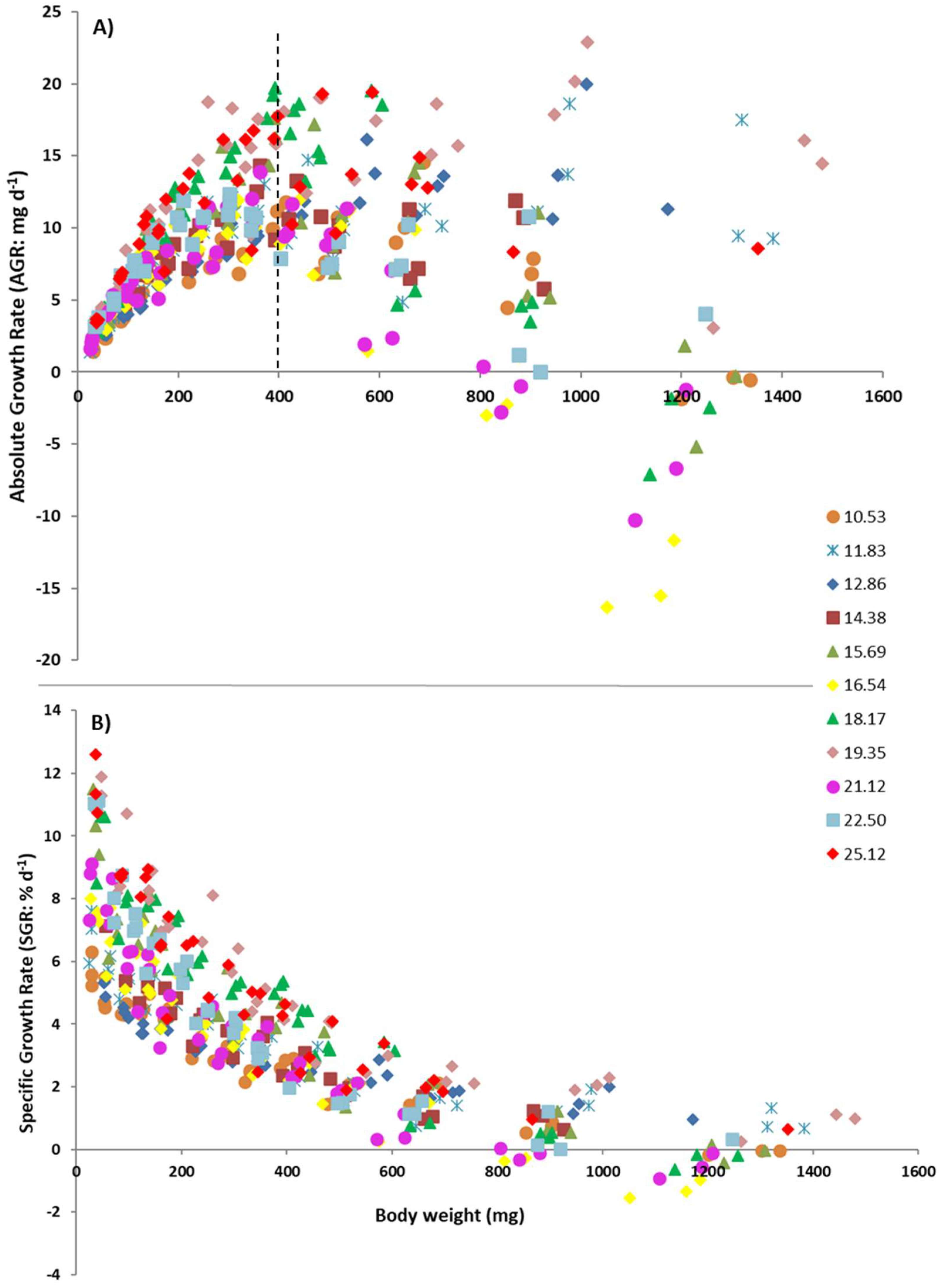
3.1. Modeling Relationships between Variables

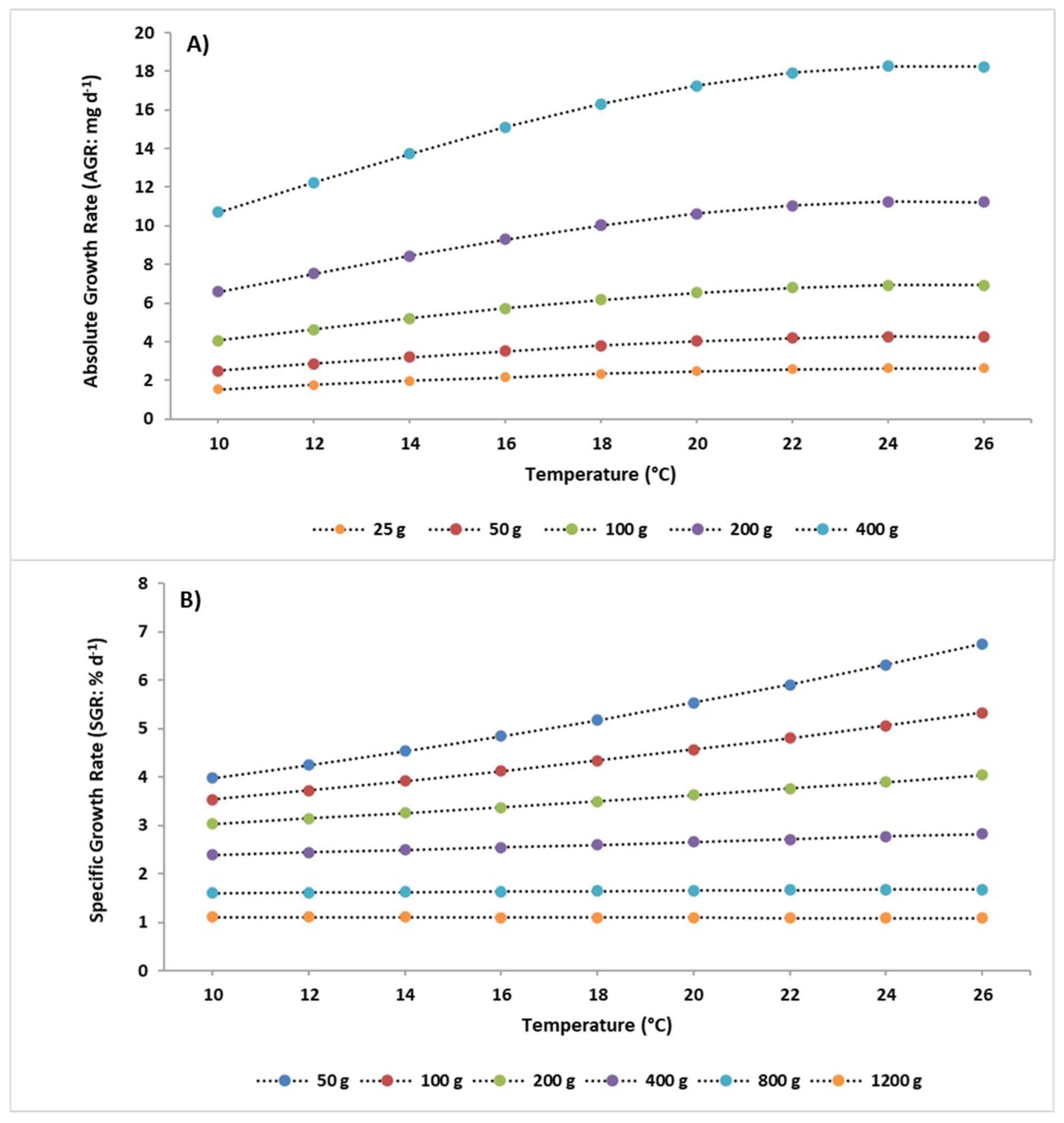
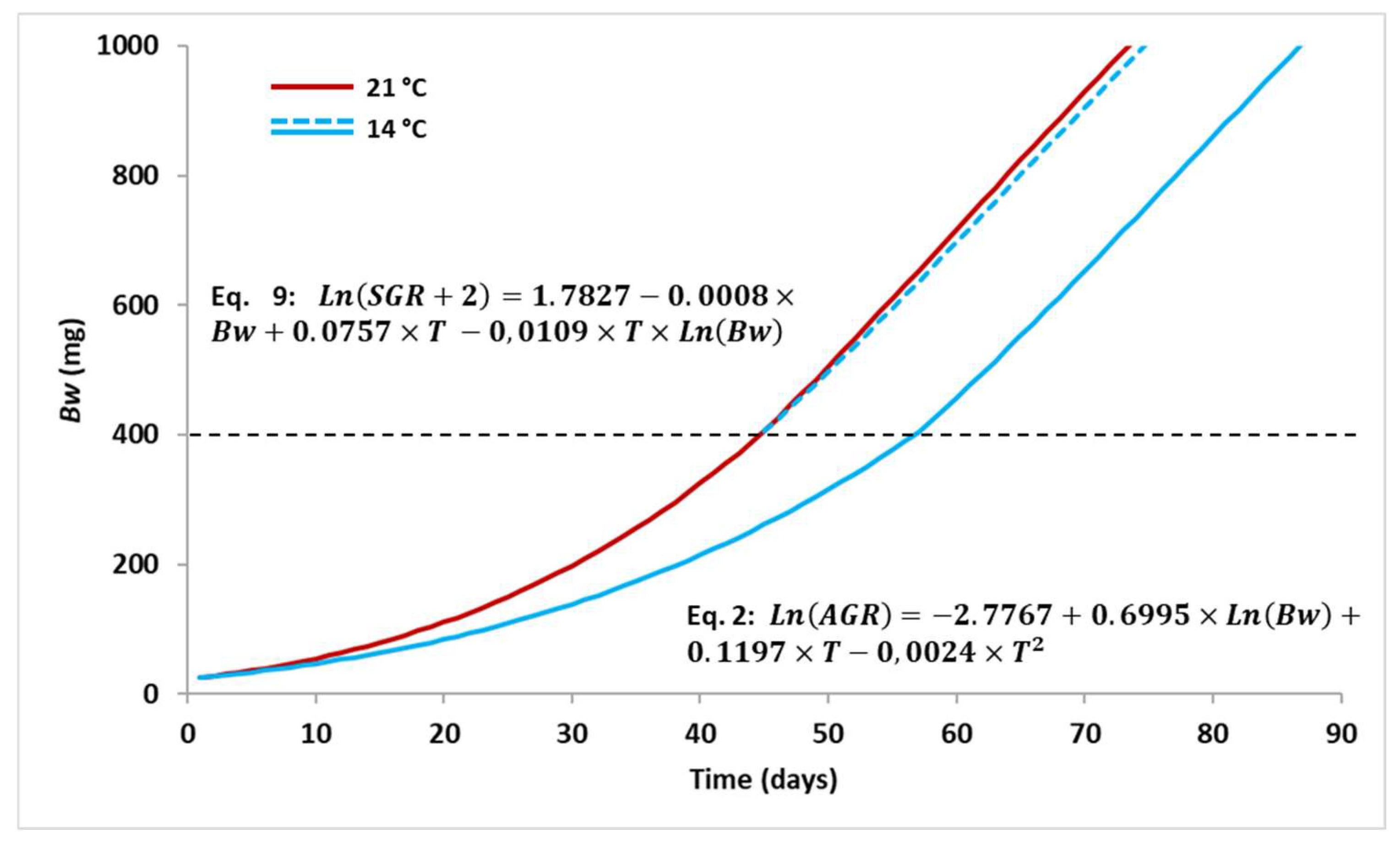
For the whole dataset, the Pearson partial correlation test showed both Bw and T to be significantly correlated to SGR, but not significantly to AGR (Table 1). A first exploration of AGR and SGR data, plotting them against Bw, showed a discontinuity in the AGR–Bw relationship from a Bw value of about 400 mg (Figure 2A). No discontinuity was observed for SGR (Figure 2B). We separated AGR and SGR data into two groups: those obtained with batches whose Bw was less than 400 mg and those whose Bw was greater than 400 mg. Then, Pearson partial correlation test for AGR and SGR were calculated for both groups of data separately (Table 1). The Pearson partial correlation test including only those Bw values less than 400 mg revealed that both Bw and T were significantly correlated to AGR and SGR. For Bw values greater than 400 mg, Bw was significantly correlated to AGR and SGR, but T was not.

Consistent with the Pearson partial correlation test results, multiple regression analysis was run for all SGR data, with Bw and T as independent variables according to the aforementioned starting model. For AGR and SGR data obtained with batches of HD whose Bw was less than 400 mg, multiple regression analysis was run with Bw and T as independent variables; while for AGR and SGR data obtained with batches of HD whose Bw was greater than 400 mg, simple linear regression was run with Bw as an independent variable. In those cases where either AGR or SGR was negative, their natural log would not exist. To avoid this, we added the positive number immediately above the lower observed negative growth value to all the calculated values, and then run the multiple regression analysis, according to Underwood [27].

For AGR and SGR from Bw values less than 400 mg, multiple regression analysis revealed that the term T × Bw was the only nonsignificant term in Equations (1) and (3) (

Table 2. Multiple regression analysis results for AGR and SGR as dependent variables from Bw values less than 400 mg. S.E., standard error; R.S.E., residual standard error; and R²adj, adjusted coefficient of determination.

AGR	Intercept a S.E. p-Level	Bw b S.E. p-Level	T c S.E. p-Level	T2 d S.E. p-Level	T Bw e S.E. p-Level	R.S.E. R2adj	ANOVA F p-Level
Equation (1)	−3.1213 0.3310 ***	0.7709 0.0584 ***	0.1396 0.260 ***	−0.0024 0.0005 ***	−0.0042 0.0033 n.s.	0.1759 90.3%	564.1 ***
Equation (2)	−2.7767 0.1886 ***	0.6995 0.0154 ***	0.1197 0.0208 ***	−0.0024 0.0005 ***	—	0.1761 90.3%	749.7 ***
Equation (3)	1.3009 0.3736 ***	−0.2181 0.0659 **	0.1739 0.0294 ***	−0.0028 0.0006 ***	−0.0072 0.0037 n.s.	0.1986 70.4%	144.8 ***
Equation (4)	1.8927 0.2138 ***	−0.3406 0.0175 ***	0.1398 0.0236 ***	−0.0029 0.0006 ***	—	0.1997 70.4%	749.7 ***
Equation (1): Ln(AGR) = Ln(a) + b·Ln(Bw) + c·T + d·T2 + e·T·Ln(Bw) Equation (2): Ln(AGR) = Ln(a) + b·Ln(Bw) + c·T + d·T2 Equation (3): Ln(SGR) = Ln(a) + b·Ln(Bw)+c·T + d·T2 + e·T·Ln(Bw) Equation (4): Ln(SGR) = Ln(a) + b·Ln(Bw) + c·T + d·T2

*** p < 0.001; ** p < 0.01; n.s. nonsignificant.

). This interaction term was removed from both equations. Then, all terms were significant in the resulting Equations (2) and (4) for which the explained variability was 90.3% for AGR and 70.1% for SGR. In Equation (2), both terms Bw and T were positive; this means that AGR increases as both independent variables do. In Equation (4), Bw coefficient was positive and T coefficient was negative; this means that SGR decreases as Bw increases, but SGR increases as T does. In both Equations (2) and (4), the term T2 was negative; this means that AGR and SGR increase as T does, but only up to a certain value of T, from which AGR and SGR decrease.

For AGR and SGR from Bw values greater than 400 mg, SLR showed the term Bw to be significant and negative in both Equations (5) and (6) (

Table 3. Simple linear regression for AGR and SGR as dependent variables from Bw values greater than 400 mg. S.E., standard error; R.S.E., residual standard error; and R², coefficient of determination.

	Intercept a S.E. p-Level	Bw b S.E. p-Level	R.S.E. R2	ANOVA F p-Level
Equation (5)	3.7852 0.0652 ***	−0.1335 0.1010 ***	0.4458 54.6%	177.7 ***
Equation (6)	6.3971 0.4425 ***	−0.7977 0.0684 ***	0.3027 48.4%	138.8 ***
Equation (5): Ln(AGR + 17) = Ln(a) + b·Ln(Bw) Equation (6): Ln(SGR + 2) = Ln(a) + b·Ln(Bw)

*** p < 0.001; n.s. nonsignificant.

); this means that, from a Bw greater than 400 mg, AGR and SGR tend to decrease as Bw increases. The variance explained by the models was 54.6% for AGR and 48.4% for SGR—both quite lower than the variances explained by the equations obtained for Bw less than 400 mg.

Multiple regression analysis for SGR showed that the term T² was not significant in Equation (7) (

Table 4. Multiple regression analysis results for SGR as dependent variable for the full dataset. S.E., standard error; R.S.E., residual standard error; and R²adj, adjusted determination coefficient.

	Intercept a S.E. p-Level	Bw b S.E. p-Level	T c S.E. p-Level	T2 d S.E. p-Level	T Bw e S.E. p-Level	R.S.E. R2adj	ANOVA F p-Level
Equation (7)	2.3010 0.3675 ***	−0.1937 0.0547 ***	0.1206 0.0308 ***	−0.0006 0.0007 n.s.	−0.0144 0.0031 ***	0.2639 72.9%	260.6 ***
Equation (8)	2.4899 0.3057 ***	−0.1933 0.0547 ***	−0.09716 0.0175 ***	—	−0.0144 0.0031 ***	0.2639 72.9%	347.3 ***
Equation (9)	1.7827 0.0526 ***	−0.0008 0.0001 ***	0.0757 0.0075 ***	—	−0.0109 0.0012 ***	0.2221 80.8%	542.6 ***
Equation (7): Ln(SGR + 2) = Ln(a) + b·Ln(Bw) + c·T + d·T2 + e·T·Ln(Bw) Equation (8): Ln(SGR + 2) = Ln(a) + b·Ln(Bw) + c·T + e·T·Ln(Bw) Equation (9): Ln(SGR + 2) = Ln(a) + b·Bw + c·T + e·T·Ln(Bw)

*** p < 0.001; n.s. nonsignificant.

), so this was removed. Equation (8) showed all terms to be significant and R²adj to be 72.9%. In Equation (9), for which the term Bw was not natural-log transformed, all terms were also significant, and a substantial improvement of the variance explained by the model was achieved (R²adj = 80.8%). In all equations, Bw coefficient was negative; this indicates a significant trend for SGR to decrease with weight gain. Conversely, T coefficient was positive; therefore, in general, SGR was greater at higher temperatures. The coefficient of term T·Bw was also negative; this means that the optimal T for SGR decreases as Bw increases.

3.2. Simulations

The equations with better fit when estimating growth were Equation (2) (R²adj = 90.3%; Table 2) for HD weighing less than 400 mg and Equation (9) (R²adj = 80.8%; Table 4) for the full data range. Simulation with Equation (2) showed optimum AGR to occur at 24.9 °C regardless of Bw; above this temperature, AGR tended to diminish (Figure 4A). Simulation with Equation (9) showed that, above a Bw of 1050 mg, SGR decreases as T increases (Figure 4B). For Bw greater than 400 mg, the variance explained was low with both Equations (5) and (6) (AGR 54.6% and SGR 48.4%, respectively; Table 3); within that weight range, the use of Equation (9) is therefore preferable to make estimates.

According to the results and to exemplify tentative production approaches managing culture conditions—specifically water temperature—the simulations shown below (Figure 5) were performed using Equation (2) to estimate individual growth starting from an initial weight of 25 mg up to a weight of 400 mg, and Equation (9) to estimate individual growth from 400 mg to a final weight of 1000 mg at different temperature regimes. In search of a balance between optimal growth and minimum mortality, we chose to use a medium-high temperature (21 °C) instead of the estimated optimal one (24.9 °C) for the individual growth simulations. To compare the duration of individual growth to a final size of 1000 mg at high temperature with that of low temperatures or at combinations of both, simulations were performed at the following temperature regimes: (i) constant temperature of 21.0 °C for the full rearing period; (ii) 21.0 °C from 25 mg up to 400 mg and 14.0 °C from 400 mg to 1000 mg; and (iii) constant temperature of 14.0 °C for the full rearing cycle.

Individual growth simulations (Figure 5) showed that a Bw of 400 mg would be reached after 44 days at 21.0 °C, or after 57 days at 14 °C; from 400 mg, a final weight of 1000 mg would be reached after 30 additional days (74 days in total) at 21.0 °C, and after 31 additional days (75 days in total) at 14.0 °C. If the complete cycle were to be performed at 14.0 °C, 400 mg would be reached after 57 days, and the final weight of 1000 mg would be reached after 31 additional days (88 days in total).

4. Discussion

Our results reveal HD growth to be influenced by T and Bw, in general terms, following the expected pattern: growth increased with T increase; when expressed in an absolute way (AGR), growth increased as Bw increased; and when expressed in a relative way (SGR), growth decreased as Bw increased. A change in the growth pattern was observed from an individual Bw of about 400 mg. Simulations with the selected models helped to explain in more detail the effect of both variables on growth.

Below 400 mg, optimum T for HD growth was 24.9 °C; above this T value, growth decreased. This result contrasts with the results obtained by Ivleva [31] in the Black Sea, indicating the optimum temperature for HD growth to be 19 °C. However, this difference may respond to the different latitudinal temperature regimes and their influence on local populations [1,32]. Galasso et al. [19] studied the metabolic rate in HD and predicted the growth rate to increase with temperature, with expected values of 7–10% d⁻¹ in the range of 15–20 °C. These values are close to ours for T range and similar to ours for Bw. Virtually all works that have studied growth of HD fed on aquaculture feed have been performed within very narrow Bw ranges, or at very specific T [22,23,24]. Moreover, rearing conditions (salinity, density and sediment type) are quite different between those studies and ours, making comparison difficult. Our results indicate that optimum T for growth changes with Bw: optimum T is lower for larger individuals, and from a Bw of around 1000 mg, growth decreases as T increases. Although HD is an eurythermal species [1] and estimated optimal T for growth can be high for certain individual Bw (24.9 °C in our experimental conditions), our results show that mortality tends to increase from a T above 22 °C, especially for individuals with a Bw higher than 400 mg. It is known that thermal stress and the resulting increased mortality in HD is related to potential heavy metal toxicity [33]. Therefore, special care must be taken in temperature management and sediment chemistry for the cultivation of this species. Another environmental variable which also plays a significant role in heavy metal toxicity and the development of HD, and could have a relevant influence on the production of this species, is salinity [21,33]. A study on the combined effect of temperature and salinity on the growth and mortality of HD is considered necessary.

The asymptotic point in growth pattern that we found at a Bw of around 400 mg may be related to sexual maturation and the type of feed used. As in most invertebrates, reproduction in HD involves alterations in feeding mediated by the neuroendocrine system that involve cessation of feeding in the final stages of gonadal maturation, followed by tissue lysis during gamete release, and finally death [1]. Hence, it might be expected that anticipation of the reproductive phase could lead to a setback in growth. In addition, growth increases when feeding HD with fish feed compared with using other feed sources [2,3]; this can be due to the high protein content in fish feed. Batista et al. [34] observed an early sexual maturation in HD fed with gilthead seabream (Sparus aurata) dry feed, a feed similar to the one used in the present study. Likewise, Pombo et al. [15] suggested that enhanced growth in HD caused by aquaculture feed may affect its normal timing of reproductive development, causing an advancement of breeding in individuals of small size. Similarly, Nesto et al. [22] showed that a diet rich in protein, such as fish feed, promotes not only a high growth rate, but also an advancement of the gametogenesis, leading to earlier sexual maturity. Considering that HD is a monotelic species that dies after breeding [1], the type of feed used in our trials might have favored not only the huge growth variability observed in Bw classes greater than 400 mg (including in some cases weight loss in sizes above 800 mg), but also the increased mortality above this Bw as a result of early reproduction. Mortality could even have been enhanced with a temperature above the tolerance threshold of the species, which depends on acclimation capacity [35] and seems to be lower the larger the individuals are—which is in line with our observations.

Simulations of individual growth (Figure 4) show that growth of up to 400 mg was faster at 21 °C. The estimated weight increase is in agreement with the results obtained by Nesto et al. [22] from individuals of the same initial Bw (25 mg) at the same density (1000 ind. m⁻²) fed on a similar fish feed, but at a temperature of 19.0 °C. However, from 400 mg to 1000 mg, simulations reveal that the influence of T on growth rate seems to have little relevance in operational terms. However, the potential influence of T on sexual maturation and mortality for this weight range is more significant from a production management point of view. This is the reason why we chose not to lower T when simulating growth above 400 mg—over that weight, mortality is lower at lower T—as a progressive change in T is also related to early breeding in polychaetes [7], and this would impair growth and favor reproduction, and hence, mortality.

To achieve the best growth and reproductive control (preventing or facilitating), key environmental variables, such as temperature and photoperiod, must be managed correctly [7,16]. Diet composition can also play a key role; a diet low in lipids can slow down early maturation in HD [15,36], while a diet high in protein content can initiate earlier gametogenesis processes and earlier sexual maturity stages [22,37]. Using fish feed to rear HD is standard practice under experimental conditions. However, this type of feed is too expensive to be used by the worm industry, although its use to stimulate breeding could be cost effective [22]. Growth modeling uses data over discrete time periods obtained from individuals or groups of individuals growing under certain relevant environmental conditions. Most growth models developed for aquaculture species only include those variables whose influence on growth is most relevant (body weight and water temperature), while other variables remain constant [38,39]. However, the type of diet used could have a significant influence on the results. Therefore, nutrition must be optimized according to production objectives, and modeling tools must be developed to assist ragworm farming. Intensive HD production can be focused on either biomass production or production of individuals of a given marketable size. For either, control of reproduction and larval availability are required. Our results demonstrated that growth and reproduction may be compromised from a size of around 400 mg if environmental conditions or nutrition are not fit for purpose.

5. Conclusions

This study revealed the strong influence of temperature on HD growth, and that from a body weight of around 400 mg, the development of the species could be modulated according to production needs to direct it towards increasing biomass or promoting reproduction by also managing other variables such as feed type and/or photoperiod. The simulations demonstrated the huge usefulness of growth modelling for production planning, making it a tool that can be used in the production of the species.

References

1. Scaps, P. A review of the biology, ecology and potential use of the common ragworm Hediste diversicolor (O.F. Müller) (Annelida: Polychaeta). Hydrobiologia 2002, 470, 203–218. [Google Scholar] [CrossRef]
2. Fidalgo e Costa, P.; Narciso, L.; Cancela da Fonseca, L. Growth, survival and fatty acid profile of Nereis diversicolor (O. F. Muller, 1776) fed on six different diets. Bull. Mar. Sci. 2000, 67, 337–343. [Google Scholar]
3. Santos, A.; Granada, L.; Baptista, T.; Anjos, C.; Simões, T.; Tecelão, C.; Fidalgo e Costa, P.; Costa, J.L.; Pombo, A. Effect of three diets on the growth and fatty acid profile of the common ragworm Hediste diversicolor (O.F. Müller, 1776). Aquaculture 2016, 465, 37–42. [Google Scholar] [CrossRef]
4. Marques, B.; Calado, R.; Lillebø, A.I. New species for the biomitigation of a super-intensive marine fish farm effluent: Combined use of polychaete-assisted sand filters and halophyte aquaponics. Sci. Tot. Environ. 2017, 599–600, 1922–1928. [Google Scholar] [CrossRef] [PubMed]
5. Pajand, Z.O.; Soltani, M.; Bahmani, M.; Kamali, A. The role oof polychaete Nereis diversicolor in bioremediation of wastewater and its growth performance and fatty acid composition in an integrated culture system with Huso huso (Linnaeus, 1758). Aquac. Res. 2017, 48, 5271–5279. [Google Scholar] [CrossRef]
6. Gilbert, F.; Kristensen, E.; Aller, R.C.; Banta, G.T.; Archambault, P.; Belley, R.; Bellucci, L.G.; Calder, L.; Cuny, P.; de Montaudouin, X.; et al. Sediment reworking by the burrowing polychaete Hediste diversicolor modulated by environmental and biological factors across the temperate North Atlantic. A tribute to Gaston Desrosiers. J. Exp. Mar. Biol. Ecol. 2021, 541, 151588. [Google Scholar] [CrossRef]
7. Wang, H.; Hagemann, A.; Reitan, K.I.; Ejlertsson, J.; Wollan, H.; Handå, A.; Malzahn, A.M. Potential of the polychaete Hediste diversicolor fed on aquaculture and biogas side streams as an aquaculture food source. Aquac. Environ. Interac. 2019, 11, 551–562. [Google Scholar] [CrossRef] [Green Version]
8. García-Alonso, J.; Müller, C.T.; Hardege, J.D. Influence of food regimes and seasonality on fatty acid composition in the ragworm. Aquat. Biol. 2008, 4, 7–13. [Google Scholar] [CrossRef] [Green Version]
9. Yousefi-Garakouei, M.; Kamali, A.; Soltani, M. Effects of rearing density on growth, fatty acid profile and bioremediation ability of polychaete Nereis diversicolor in an integrated aquaculture system with rainbow trout (Oncorhynchus mykiss). Aquac. Res. 2019, 50, 725–735. [Google Scholar] [CrossRef]
10. Jerónimo, D.; Lillebø, A.I.; Santos, A.; Cremades, J.; Calado, R. Performance of polychaete assisted sand filters under contrasting nutrient loads in an integrated multi-trophic aquaculture (IMTA) system. Sci. Rep. 2020, 10, 20871. [Google Scholar] [CrossRef]
11. Luis, O.J.; Ponte, A.C. Control of reproduction of the shrimp Penaeus kerathurus held in captivity. J. World Aquac. Soc. 1993, 24, 31–39. [Google Scholar] [CrossRef]
12. Cardinaletti, G.; Mosconi, G.; Salvatori, R.; Lanari, D.; Tomassoni, D.; Carnevali, O.; Polzonetti-Magni, A.M. Effect of dietary supplements of mussel and polychaetes on spawning performance of captive sole, Solea solea (Linnaeus, 1758). Animal Reprod. Sci. 2009, 113, 167–176. [Google Scholar] [CrossRef] [PubMed]
13. Durou, C.; Poirier, L.; Amiard, J.C.; Budzinski, H.; Gnassia-Barelli, M.; Lemenach, K.; Peluhet, L.; Mouneyrac, C.; Roméo, M.; Amiard-Triquet, C. Biomonitoring in a clean and a multi-contaminated estuary based on biomarkers and chemical analyses in the endobenthic worm Nereis diversicolor. Environ. Poll. 2007, 148, 445–458. [Google Scholar] [CrossRef]
14. Barrick, A.; Marion, J.M.; Perrein-Ettajani, H.; Châtel, A.; Mouneyrac, C. Baseline levels of biochemical biomarkers in the endobenthic ragworm Hediste diversicolor as useful tools in biological monitoring of estuaries under anthropogenic pressure. Mar. Poll. Bull. 2018, 129, 81–85. [Google Scholar] [CrossRef] [PubMed]
15. Pombo, A.; Baptista, T.; Granada, L.; Ferreira, S.M.F.; Gonçalves, S.C.; Anjos, C.; Erica, S.A.; Chainho, P.; Cancela da Fonseca, L.; Fidalgo e Costa, P.; et al. Insight into aquaculture’s potential of marine annelid worms and ecological concerns: A review. Rev. Aquac. 2020, 12, 107–121. [Google Scholar] [CrossRef]
16. Olive, P.J.W. Polychaete aquaculture and polychaete science: A mutual synergism. Hydrobiologia 1999, 402, 175–183. [Google Scholar] [CrossRef]
17. Mayer, P.; Estruch, V.; Blasco, J.; Jover, M. Predicting the growth of gilthead sea bream (Sparus aurata L.) farmed in marine cages under real production conditions using temperature- and time-dependent models. Aquac. Res. 2008, 39, 1046–1052. [Google Scholar] [CrossRef]
18. Mayer, P.; Estruch, V.; Martí, P.; Jover, M. Use of quantile regression and discriminant analysis to describe growth patterns in farmed gilthead sea bream (Sparus aurata). Aquaculture 2009, 292, 30–36. [Google Scholar] [CrossRef]
19. Galasso, H.L.; Richard, M.; Lefebvre, S.; Aliaume, C.; Callier, M.D. Body size and temperature effects on standard metabolic rate for determining metabolic scope for activity of the polychaete Hediste (Nereis) diversicolor. PeerJ 2018, 6, e5675. [Google Scholar] [CrossRef] [Green Version]
20. Hernández, J.M.; Gasca-Leyva, E.; León, C.J.; Vergara, J.M. A growth model for gilthead seabream (Sparus aurata). Ecol. Model. 2003, 165, 265–283. [Google Scholar] [CrossRef]
21. Bagarrão, R.; Fidalgo e Costa, P.; Baptista, T.; Pombo, A. Reproduction and growth of polychaete Hediste diversicolor (OF Müller, 1776) under different environmental conditions. In Proceedings of the International Meeting on Marine Research 2014, Peniche, Portugal, 10–11 July 2014. [Google Scholar] [CrossRef]
22. Nesto, N.; Simonini, R.; Prevedelli, D.; da Ros, L. Effects of diet and density on growth, survival and gametogenesis of Hediste diversicolor (O.F. Müller, 1776) (Nereididae, Polychaeta). Aquaculture 2012, 362–363, 1–9. [Google Scholar] [CrossRef]
23. Fidalgo e Costa, P. Reproduction and growth in captivity of the polychaete Nereis diversicolor O. F. Muller, 1776, using two different kinds of sediment: Preliminary assays. Bol. Inst. Esp. Oceanog. 1999, 15, 351–355. [Google Scholar]
24. Nielsen, A.M.; Eriksen, N.T.; Lonsmann Iversen, J.J.; Riisgard, H.U. Feeding, growth and respiration in the polychaetes Nereis diversicolor (facultative filter-feeder) and N. virens (omnivorous)—A comparative study. Mar. Ecol. Prog. Ser. 1995, 125, 149–158. [Google Scholar] [CrossRef] [Green Version]
25. Rasines, I.; Martín, I.; Aguado-Giménez, F. Contribution to the intensive cultivation of Hediste diversicolor. In Proceedings of the Aquaculture Europe International Conference and Exposition, Funchal, Portugal, 4–7 October 2021. [Google Scholar]
26. García-García, B.; Cerezo-Valverde, J.; Aguado-Giménez, F.; García-García, J.; Hernández, M.D. Effect of the interaction between body weight and temperature on growth and maximum daily food intake in sharpsnout sea bream (Diplodus puntazzo). Aquacult. Int. 2010, 19, 131–141. [Google Scholar] [CrossRef]
27. Underwood, A.J. Experiments in Ecology. Their Logical Design and Interpretation Using Analysis of Variance; Cambridge University Press: Cambridge, UK, 1997. [Google Scholar]
28. Aguado-Giménez, F.; García-García, B. Growth and food intake models in Octopus vulgaris Cuvier (1797): Influence of body weight, temperature, sex and diet. Aquacult. Int. 2002, 10, 361–377. [Google Scholar] [CrossRef]
29. Miliou, H.; Fintikaki, M.; Kountouris, T.; Verriopoulos, G. Combined effects of temperature and body weight on growth and protein utilization of the common octopus, Octopus vulgaris. Aquaculture 2005, 249, 245–256. [Google Scholar] [CrossRef]
30. Lin, X.; Xie, S.; Su, Y.; Cui, Y. Optimum temperature for the growth performance of juvenile orange spotted grouper (Epinephelus coioides H.). Chin. J. Oceanol. Limnol. 2008, 26, 69–75. [Google Scholar] [CrossRef] [Green Version]
31. Ivleva, I.V. The influence of temperature on the transformation of matter in marine invertebrates. In Marine Food Chains; Steele, J.H., Ed.; Oliver and Boyd: Edinburgh, UK, 1970; pp. 96–112. [Google Scholar]
32. Arias, A.M.; Drake, P. Distribution and production of the polychaete Nereis diversicolor in a shallow coastal lagoon in the Bay of Cádiz. Cahiers Biol. Mar. 1995, 36, 201–210. [Google Scholar]
33. Ozoh, P.T.E. The effect of temperature and salinity on copper body-burden and copper toxicity to Hediste (Nereis) diversicolor. Environ. Monit. Assess. 1992, 21, 11–17. [Google Scholar] [CrossRef]
34. Batista, F.M.; Fidalgo e Costa, P.; Ramos, A.; Passos, A.M.; Pousao Ferreira, P.; Cancela da Foseca, L. Production of the ragworm Nereis diversicolor (O.F. Müller, 1776), fed with a diet for gilthead seabream Sparus aurata L.; 1758: Survival, growth, feed utilization and oogenesis. Bol. Inst. Esp. Oceanog. 2003, 19, 447–451. [Google Scholar]
35. Fernandes, F.; Jerónimo, D.; Diniz, M.; Calado, R.; Madeira, D. Cellular stress response and thermal tolerance limits of the ragworm Hediste diversicolor under global change scenarios. In Proceedings of the ICYMARE—International Conference for Young Marine Researchers, Bremen, Germany, 24–27 September 2019. [Google Scholar] [CrossRef]
36. Machado, D.; França, M.; Pombo, A.; Anjos, C.M.; Ferreira, S.M.; Gonçalves, S.C.; Costa, P.F.; Costa, J.V.; Baptista, T.M. Effect of different diets on growth of Hediste diversicolor (O. F. Müller, 1776) (Nereididae, Polychaeta) juveniles. In Proceedings of the International Meeting on Marine Research 2016, Peniche, Portugal, 14–15 July 2016. [Google Scholar] [CrossRef]
37. Jerónimo, D.; Lillebø, A.I.; Rey, F.; Koga Li, H.; Domingues, M.R.M.; Calado, R. Optimizing the timeframe to produce polychaetes (Hediste diversicolor) enriched with esssential fatty acids under different combinations of temperatura and salinity. Front. Mar. Sci. 2021, 8, 671545. [Google Scholar] [CrossRef]
38. Björnsson, B.; Seteinarsson, A.; Árnason, T. Growth model for Atlantic cod (Gadus morhua): Effects of temperature and body weight on growth rate. Aquaculture 2007, 271, 216–226. [Google Scholar] [CrossRef]
39. Dumas, A.; France, J.; Bureau, D. Modelling growth and body composition in fish: Where have we been and where are we going? Aquac. Res. 2010, 41, 161–181. [Google Scholar] [CrossRef]
Figure 1. (A) Experimental units (height 20 cm; internal diameter 11.3 cm) and (B) RAS, including six polycarbonate trays (width 35 cm; height 30 cm; length 54 cm) in which 6–7 experimental units were placed.
Aquacj 03 00004 g001
Figure 2. Plots of all (A) AGR and (B) SGR observed data for Bw and T tested in the growth assays. Vertical dotted line in A indicates the Bw value above which dispersion of AGR values is apparent.
Aquacj 03 00004 g002
Figure 3. Mean mortality (M) observed in different (A) weight classes and (B) temperatures (bars = standard error).
Aquacj 03 00004 g003
Figure 4. (A) Estimation of AGR (Equation (2)) for individuals weighing less than 400 mg and (B) estimation of SGR (Equation (9)) for individuals in the full range of observed weight at different temperatures within the range of observed temperatures.
Aquacj 03 00004 g004
Figure 5. Simulation of individual Bw increases using the best-fitting equations under different temperature regimes, starting from 25 mg up to a final Bw of 1000 mg.
Aquacj 03 00004 g005