Controllability of a Class of Heterogeneous Networked Systems

Abstract

This paper examines the controllability of a class of heterogeneous networked systems where the nodes are linear time-invariant systems (LTI), and the network topology is triangularizable. The literature contains necessary and sufficient conditions for the controllability of such systems where the control input matrices are identical in each node. Here, we extend this result to a class of heterogeneous systems where the control input matrices are distinct in each node. Additionally, we discuss the controllability of a more general system with triangular network topology and obtain necessary and sufficient conditions for controllability. Theoretical results are supplemented with numerical examples.

1. Introduction

The controllability of networked dynamical systems remains one of the most challenging problems in the field of control theory. The prevalence of networks of dynamical systems in numerous engineering and technology fields supports the rising emphasis placed on the controllability of networked systems [1,2,3]. In System and Control literature, there are different notions of controllability, including state controllability, structural controllability, etc. The classical idea of controllability, introduced by R. E. Kalman [4] in the 1960s, deals with the ability of a single high-dimensional system to steer itself from an arbitrary initial state to a desired final state, whereas, structural controllability, introduced by Lin [5] in 1974, attempts to obtain some numerical values for the parameters in system matrices describing the system’s dynamics so that it is controllable in the sense of Kalman. Using rank conditions, spectral features, graph-theoretic properties, etc., many authors have explored controllability criteria for such systems over the past few decades [6,7,8,9,10,11,12,13]. The traditional theory of control paved the way for an advanced approach applicable to complex networks with more than one interconnected dynamical system. With time, it was evident that modelling complicated real-life systems required large-scale networks, and the controllability of such systems became unavoidable [14,15,16,17].

Over the years, several approaches have been employed to study the controllability of a dynamical system. Zhou [18] studied the controllability and observability of networked systems having different dynamics in each subsystem. Based on the Popov–Belevitch–Hautus(PBH) test, he obtained some necessary and sufficient conditions for controllability which depended upon the dynamics of the subsystems and the network topology. Wang et al. [19] proposed a set of necessary conditions for the controllability of a homogeneous LTI networked system that required solving matrix equations. Additionally, conditions were derived that can be used to analyze the controllability of the networked system based on network topology, node dynamics, external control inputs, and inner interactions. In Wang L. et al. [19], the interactions between connected nodes are performed through high-dimensional inputs and outputs of the node dynamics. Later, Wang L. et al. [20] studied the controllability of homogeneous networked LTI systems having one-dimensional communication. They obtained a necessary and sufficient condition for the controllability of such systems along with some controllability results over specific network topologies, such as a chain, tree, star, etc. A relatively simple, less computational method for the controllability of homogeneous networked LTI systems was given by Hao et al. [21] in 2018 using spectral properties. Compared with Wang L. et al. [19], the conditions are easy to verify as they do not involve solving matrix equations. All these works discussed the controllability of a networked system with nodes having identical dynamics. However, in real-life situations, the individual nodes may not always have the same dynamics. Controllability of networked systems with heterogeneous dynamics poses a fascinating challenge as the intrinsic dynamics of individual nodes add to the complexity contributed by the network topology. Wang P. et al. [22] tried to extend the results obtained by Wang L. et al. [19] that were for homogeneous systems to heterogeneous systems. Some necessary conditions for controllability were obtained based on the network topology and the subsystem dynamics. Based on this work, Xiang et al. [23] derived necessary and sufficient conditions for controllability of a particular class of heterogeneous systems. Based on the results of Xiang et al. [23], Ajayakumar et al. [24] derived some necessary conditions for the controllability of heterogeneous systems. Using the idea of the determinant factor and the Smith normal form, a necessary and sufficient condition for controllability was derived by Kong et al. [25] for a general heterogeneous networked system. However, the result is difficult to verify as it involves significant computation. Ajayakumar et al. [26] extended the result of Hao et al. [21] that was for the controllability of homogeneous systems to a particular class of heterogeneous systems with identical control input matrices.

In this work, we extend the result in [26] to a class of heterogeneous networked systems, where the control input matrix is non-identical in each node. We also examine the controllability of a more general heterogeneous networked system over some specific network topologies. Necessary and sufficient conditions for the controllability of such systems are obtained. The rest of the paper is arranged as follows. Some preliminary information is given in Section 2. The controllability problem is formulated in Section 3. Section 4 presents the necessary and sufficient conditions for the controllability of the heterogeneous networked system formulated in Section 3. It also provides some controllability results over some specific topologies. Examples are provided to substantiate the derived results. Section 5 concludes the study and outlines the future scope of the research.

2. Preliminaries

In this paper, we use the following notations. I denotes the identity matrix and $\{e_1,e_2,\dots ,e_n\}$ represents the canonical basis for ${\mathbb{R}}^n$. Let $diag\{a_1,a_2,\dots ,a_n\}$ denote diagonal matrix of order n with diagonal entries $a_1,a_2,\dots ,a_n$, and $uppertriang\{a_1,a_2,\dots ,a_n\}$ denotes an upper triangular matrix of the form

$$\left[\begin{array}{ccccc}{a}_1& *& *& \dots & *\\ 0& a_2& *& \dots & *\\ 0& 0& a_3& \dots & *\\ ⋮& ⋮& ⋮& \ddots & ⋮\\ 0& 0& 0& \dots & a_n\end{array}\right]$$

Let $\sigma \left(A\right)$ denotes the eigen spectrum of a matrix A. The following lemmas will be used in the subsequent sections of this paper.

Lemma 1

([27]). Let A and B be similar matrices, that is, there exists a non-singular matrix P, such that $PB{P}^{-1}=A$. If ν is a left eigenvector of A with respect to the eigenvalue λ, then $\nu P$ is an eigenvector of B with respect to the eigenvalue λ.

Lemma 2

([28]). Let $A\otimes B$ denotes the Kronecker product of two matrices A and B. We use the following properties of Kronecker product in this paper.

(i) 

$(A\otimes B)(C\otimes D)=(AC\otimes BD)$.

(ii) 

${(A\otimes B)}^{-1}=A^{-1}\otimes B^{-1}$ if A and B are invertible.

(iii) 

$(A+B)\otimes C=A\otimes C+B\otimes C$.

(iv) 

$A\otimes (B+C)=A\otimes B+A\otimes C$.

(v) 

$A\otimes B=0$ if and only if $A=0$ or $B=0$.

Lemma 3

([29]). A linear time-invariant control system characterized by the pair of matrices $(A,B)$ is controllable if, and only if, left eigenvectors of A are not orthogonal to columns of B, i.e., $\nu A=\lambda \nu$ implies that $\nu B\ne 0$.

3. Model Formulation

Consider a heterogeneous networked linear time-invariant system with N nodes, where the $i^{th}$ node is described by the following differential equation:

$$\dot{x_i}\left(t\right)=A_i{x}_i\left(t\right)+\sum _{j=1}^N{c}_{ij}H{x}_j\left(t\right)+d_i{B}_i{u}_i\left(t\right),i=1,2,\dots ,N$$

(1)

where, $x_i\left(t\right)\in {\mathbb{R}}^n$ is the state vector and $u_i\left(t\right)\in {\mathbb{R}}^m$ is the external control vector. $A_i$ is an $n\times n$ matrix and $B_i$ is an $n\times m$ matrix called the state matrix and the control matrix of node i, respectively.

$$d_i=\left\{\begin{array}{c}1,ifnodeiisundercontrol\hfill \\ 0,otherwise\hfill \end{array}\right.$$

The connection strength between the nodes i and j is given by $c_{ij}\in \mathbb{R}$. If there is a communication from node j to node i, $c_{ij}\ne 0$ and otherwise, $c_{ij}=0$, $i,j=1,2,\dots ,N$. The $n\times n$ matrix H denotes the inner coupling matrix describing the interconnections among the states $x_j,j=1,2,\dots ,N$ of the nodes.

The network topology and external input channels of the networked system (1), are given by the $N\times N$ matrices

$$C=\left[c_{ij}\right]andD=diag\{d_1,d_2,\dots ,d_N\}$$

(2)

respectively. If we denote the state matrix and the total external control input of the networked system (1) by $X={\left[x_1^T,\dots ,x_N^T\right]}^T$ and $U={\left[u_1^T,\dots ,u_N^T\right]}^T$, respectively, using the Kronecker product notation, (1) can be reduced into the following compact form:

$$\dot{X}\left(t\right)=FX\left(t\right)+GU\left(t\right)$$

(3)

with,

$$F=A+C\otimes H,G=(D\otimes I)B$$

(4)

where $A=blockdiag\{A_1,A_2,\dots ,A_N\}$ and $B=blockdiag\{B_1,B_2,\dots ,B_N\}$. If the inner coupling matrix is also different in each node, i.e., if the dynamics of the $i^{th}$ node is given by

$$\dot{x_i}\left(t\right)=A_i{x}_i\left(t\right)+\sum _{j=1}^N{c}_{ij}{H}_i{x}_j\left(t\right)+d_i{B}_i{u}_i\left(t\right),i=1,2,\dots ,N$$

(5)

the networked system can be reduced to the compact form (3), where

$$F=\left[\begin{array}{cccc}{A}_1+c_{11}{H}_1& c_{12}{H}_1& \dots & c_{1N}{H}_1\\ c_{21}{H}_2& A_2+c_{22}{H}_2& \dots & c_{2N}{H}_2\\ ⋮& ⋮& \ddots & ⋮\\ c_{N1}{H}_N& c_{N2}{H}_N& \dots & A_N+c_{NN}{H}_N\end{array}\right]$$

and $G=(D\otimes I)B$.

4. Controllability Results in a General Network Topology

Ajayakumar et al. [26] studied the controllability of (3) when the network topology is triangularizable, and the system parameter matrices satisfy certain conditions. There the control input matrices were identical in each node. Here, we will extend this result to a system where each node has different control input matrices.

We find that there exists a non-singular matrix T, such that $TC{T}^{-1}=J$, where $J=uppertriang\{{\lambda }_1,{\lambda }_2,\dots ,{\lambda }_N\}$ is the Jordan Canonical Form of C. Let $\sigma (A_i+{\lambda }_{i}H)=\{{\mu }_i^1,\dots ,{\mu }_i^{q_i}\}$ denotes the set of eigenvalues of $A_i+{\lambda }_{i}H,i=1,2,\dots ,N$ and ${\xi }_{ij}^k,k=1,\dots ,{\gamma }_{ij}$ be the left eigenvectors of $A_i+{\lambda }_{i}H$ corresponding to ${\mu }_i^j,j=1,\dots ,q_i,i=1,\dots ,N$, where ${\gamma }_{ij}\ge 1$ is the geometric multiplicity of the eigenvalue ${\mu }_i^j$. We will make use of the following theorem.

Theorem 1

([26]). Let T be the triangularizing matrix for the network topology matrix C and suppose $T\otimes I$ commutes with A. Let $({\mu }_i^j,{\xi }_{ij}^k)$ denotes the left eigenpair of $A_i+{\lambda }_{i}H$. Then the following statements hold true.

(i) 

The eigenspectrum of F is the union of eigenspectrum of $A_i+{\lambda }_{i}H$, where, $i=1,2,\dots ,N$. That is,

$$\sigma \left(F\right)={\cup }_{i=1}^N\sigma (A_i+{\lambda }_{i}H)=\{{\mu }_1^1,\dots ,{\mu }_1^{q_1},\dots ,{\mu }_N^1,\dots ,{\mu }_N^{q_N}\}$$

(ii) 

If J is a diagonal matrix, then $e_{i}T\otimes {\xi }_{ij}^k,k=1,\dots ,{\gamma }_{ij}$ are the left eigenvectors of F corresponding to the eigenvalue ${\mu }_i^j,j=1,\dots ,q_i,i=1,\dots ,N$.

(iii) 

If J contains a Jordan block of order $l\ge 2$ for some eigenvalue ${\lambda }_{i_0}$ of C with ${\xi }_{ij}^{k}H=0$ for all $i=i_0,i_0+1,\dots ,i_0+l-1,j=1,2,\dots ,q_i,k=1,2,\dots ,{\gamma }_{ij}$, then $e_{i}T\otimes {\xi }_{ij}^k,k=1,\dots ,{\gamma }_{ij}$ are the left eigenvectors of F corresponding to the eigenvalue ${\mu }_i^j,i=1,2,\dots ,N,j=1,2,\dots ,q_i$.

With the aid of the above result, we can prove the following necessary and sufficient conditions for controllability of the networked system (3).

Theorem 2.

Let T be a non-singular matrix triangularizing matrix C such that $T\otimes I$ commutes with A. If J contains a Jordan block of order $l\ge 2$ corresponding to the eigenvalue ${\lambda }_{i_0}$ of C, then assume that ${\xi }_{ij}^{k}H=0$ for all $i=i_0,i_0+1,\dots ,i_0+l-1,j=1,2,\dots ,q_i,k=1,2,\dots ,{\gamma }_{ij}$, where ${\xi }_{ij}^k,i=1,2,\dots ,N,j=1,2,\dots ,q_i,k=1,2,\dots ,{\gamma }_{ij}$ are the left eigenvectors of $A_i+{\lambda }_{i}H$ corresponding to the eigenvalues ${\mu }_i^j,i=1,2,\dots ,N,j=1,2,\dots ,q_i$. Then, the networked system (3) is controllable if, and only if,

(i) 

$e_{i}TD\ne 0$ for all $i=1,\dots ,N$

(ii) 

For a fixed i, each left eigenvector ξ of $A_i+{\lambda }_{i}H$, $\xi Bj\ne 0$ for some $j\in \{1,2,\cdots ,N\}$ with ${\left[e_{i}TD\right]}_j\ne 0$,

(iii) 

If matrices $A_{i_1}+{\lambda }_{i_1}H,A_{i_2}+{\lambda }_{i_2}H,\dots ,A_{i_p}+{\lambda }_{i_p}H({\lambda }_{i_k}\in \sigma \left(C\right),k=1,\dots ,p,wherep>1)$ have a common eigenvalue σ, then $(e_{i_1}TD\otimes {\xi }_{i_1}^1)B,\cdots ,(e_{i_1}TD\otimes {\xi }_{i_1}^{{\gamma }_{i_1}})B,\dots ,(e_{i_p}TD\otimes {\xi }_{i_p}^1)B,\dots ,(e_{i_p}TD\otimes {\xi }_{i_p}^{{\gamma }_{i_p}})B$ are linearly independent vectors, where ${\gamma }_{i_k}\ge 1$ is the geometric multiplicity of σ for $A_{i_k}+{\lambda }_{i_k}H$ and ${\xi }_{i_k}^l(l=1,\dots ,{\gamma }_{i_k})$ are the left eigenvectors of $A_{i_k}+{\lambda }_{i_k}H$ corresponding to $\sigma ,k=1,\dots ,p$.

Proof. 

(Necessary part) Fix i. Let $\xi$ be an arbitrary left eigenvector of $A_i+{\lambda }_{i}H$. From Theorem 1, we find that $e_{i}T\otimes \xi$ is a left eigenvector of F. By Lemma 3, for the networked system (3) to be controllable, we must have

$$(e_{i}T\otimes \xi )(D\otimes I)B=(e_{i}TD\otimes \xi )B\ne 0$$

This implies that $e_{i}TD\ne 0$ and $\xi B_j\ne 0$ for some $j\in \{1,2,\dots ,N\}$ with ${\left[e_{i}TD\right]}_j\ne 0$.

Now, suppose that the matrices $A_{i_1}+{\lambda }_{i_1}H,\cdots ,A_{i_p}+{\lambda }_{i_p}H({\lambda }_{i_k}\in \sigma \left(C\right),k=1,\dots ,p,$ where $p>1)$ have a common eigenvalue $\sigma$. Then the left eigenvectors of F corresponding to $\sigma$ can be expressed as a linear combination in the form ${\sum }_{k=1}^p{\sum }_{l=1}^{{\gamma }_{i_k}}{\alpha }_{kl}(e_{i_k}T\otimes {\xi }_{i_k}^l)$, where ${\alpha }_{kl}\in \mathbb{R}(k=1,\dots ,p,l=1,\dots ,{\gamma }_{i_k})$ are scalars, not all are zero and ${\xi }_{i_k}^1,\dots ,{\xi }_{i_k}^{{\gamma }_{i_k}},$ are the eigenvectors of $A_{i_k}+{\lambda }_{i_k}H$ corresponding to the eigenvalue $\sigma$, where $k=1,\dots ,p$. If the networked system is controllable, then

$$\left[\sum _{k=1}^p\sum _{l=1}^{{\gamma }_{i_k}}{\alpha }_{kl}(e_{i_k}T\otimes {\xi }_{i_k}^l)\right](D\otimes I)B\ne 0$$

Consequently, we have

$$\sum _{k=1}^p\sum _{l=1}^{{\gamma }_{ik}}{\alpha }_{kl}\left[\left(e_{i_k}TD\otimes {\xi }_{ik}^l\right)B\right]\ne 0$$

for any scalars ${\alpha }_{kl}\in \mathbb{R}(k=1,\dots ,p,l=1,\dots ,{\gamma }_{ik})$, not all of them are zero. This implies that the vectors $\left[e_{i1}TD\otimes {\xi }_{i1}^1\right)B,\dots ,\left(e_{i1}TD\otimes {\xi }_{i1}^{{\gamma }_{i1}}\right)B,\dots ,$$\left(\left(e_{ip}TD\right)\otimes \left({\xi }_{ip}^1\right)\right)B,\dots ,$$\left(e_{ip}TD\otimes {\xi }_{ip}^{{\gamma }_{ip}}\right)B$ are linearly independent in ${\mathbb{R}}^{Nn}$.

(Sufficiency part) To prove the converse part, we will show that if the networked system is uncontrollable, at least one condition in Theorem 1 does not hold. Suppose that the networked system (3) is not controllable. Then by Lemma 3, there exists a left eigenpair $(\tilde{\mu },\tilde{v})$ of F, such that $\tilde{v}G=0$.

If $\tilde{\mu }\in \sigma (A_{i_0}+{\lambda }_{i_0}H)$ and $\tilde{\mu }\notin \sigma (A_1+{\lambda }_{1}H)\cup \dots \cup \sigma (A_{i_0-1}+{\lambda }_{i_0-1}H)\cup \sigma (A_{i_0+1}+{\lambda }_{i_0+1}H)\cup \dots \cup \sigma (A_{i_N}+{\lambda }_{i_N}H)$. Again $\tilde{v}$ can be written as a linear combination, $\tilde{v}={\sum }_{l=1}^{{\gamma }_{{i_0}_{j_0}}}{\alpha }_0^l(e_{i_0}T\otimes {\xi }_{{i_0}_{j_0}}^l)$, where ${\xi }_{{i_0}_{j_0}}^1,\dots ,{\xi }_{{i_0}_{j_0}}^{{\gamma }_{{i_0}_{j_0}}}$ of left eigenvectors of $A_{i_0}+{\lambda }_{i_0}H$ corresponding to $\tilde{\mu }$, where, $\left[{\alpha }_0^1,\dots ,{\alpha }_0^{{\gamma }_{{i_0}_{j_0}}}\right]$ is some non-zero vector. Now $\tilde{v}G=0$ implies

$$\begin{array}{cc}\hfill \sum _{l=1}^{{\gamma }_{{i_0}_{j_0}}}{\alpha }_0^l(e_{i_0}T\otimes {\xi }_{{i_0}_{j_0}}^l)(D\otimes I)B& =\left[\left(e_{i_0}TD\right)\otimes \left(\sum _{l=1}^{{\gamma }_{{i_0}_{j_0}}}{\alpha }_0^l{\xi }_{{i_0}_{j_0}}^l\right)\right]B=0\hfill \end{array}$$

This implies that either $e_{i_0}TD=0$ or $\left({\sum }_{l=1}^{{\gamma }_{{i_0}_{j_0}}}{\alpha }_0^l{\xi }_{{i_0}_{j_0}}^l\right)B_j=0$ for all $j\in \{1,2,\cdots ,N\}$ with ${\left[e_{i}TD\right]}_j\ne 0$. Keep in mind that ${\sum }_{l=1}^{{\gamma }_{{i_0}_{j_0}}}{\alpha }_0^l{\xi }_{{i_0}_{j_0}}^l$ is a left eigenvector of $A_{i_0}+{\lambda }_{i_0}H$. Thus, if the networked system is uncontrollable, then either condition $\left(i\right)$ or condition $\left(ii\right)$ does not hold true.

Let $\tilde{\mu }$ be the common eigenvalue of the matrices $A_{i_1}+{\lambda }_{i_1}H,\dots ,A_{i_p}+{\lambda }_{i_p}H({\lambda }_{i_k}\in \sigma \left(C\right),$ for $k=1,\dots ,p,p>1)$. Additionally, let the eigenvectors of $A_{i_k}+{\lambda }_{i_k}H$ corresponding to $\tilde{\mu }$ are ${\xi }_{i_k}^1,\dots ,{\xi }_{i_k}^{{\gamma }_{i_k}}$, where $k=1,\dots ,p$. Since $\tilde{v}$ can be expressed in the form ${\sum }_{k=1}^p{\sum }_{l=1}^{{\gamma }_{i_k}}{\alpha }_0^{kl}\left(e_{i_k}T\otimes {\xi }_{ik}^l\right)$, where ${\alpha }_0^{kl}(l=1,\dots ,{\gamma }_{i_k},k=1,\dots ,p)$ are some scalars, which are not all zero. Then, $\tilde{v}G=0$ implies that there exists a non-zero vector $\left[{\alpha }_0^{11},\dots ,{\alpha }_0^{1{\gamma }_{i_1}},\dots ,{\alpha }_0^{p1},\dots ,{\alpha }_0^{p{\gamma }_{i_p}}\right]$, such that

$$\left[\sum _{k=1}^p\sum _{l=1}^{{\gamma }_{i_k}}{\alpha }_0^{kl}\left(e_{i_k}T\otimes {\xi }_{i_k}^l\right)\right](D\otimes I)B=\sum _{k=1}^p\sum _{l=1}^{{\gamma }_{i_k}}{\alpha }_0^{kl}\left\{\left[(e_{i_k}TD)\otimes ({\xi }_{i_k}^l)\right]B\right\}=0$$

This implies that $(e_{i_1}TD\otimes {\xi }_{i_1}^1)B,\dots ,(e_{i_1}TD\otimes {\xi }_{i_1}^{{\gamma }_{i_1}})B,\dots ,(e_{i_p}TD\otimes {\xi }_{i_p}^1)B,\dots ,(e_{i_p}TD\otimes {\xi }_{i_p}^{{\gamma }_{i_p}})B$ are linearly dependent. Thus, at least one condition in Theorem 2 does not hold true, when the networked system is uncontrollable. □

The following examples illustrate the result obtained in Theorem 2.

Example 1.

Consider a heterogeneous networked system with three nodes with the following dynamics; the state matrices and control matrices of each nodes are given by,

$$A_1=\left[\begin{array}{ccc}1& 1& 1\\ 0& 1& 1\\ 0& 0& 1\end{array}\right],A_2=A_3=\left[\begin{array}{ccc}1& 2& 1\\ 0& 1& 1\\ 1& 1& 2\end{array}\right],B_1=\left[\begin{array}{c}1\\ 0\\ 1\end{array}\right],B_2=\left[\begin{array}{c}1\\ -1\\ -1\end{array}\right],B_3=\left[\begin{array}{c}1\\ 1\\ 1\end{array}\right]$$

(6)

The network topology matrix, inner-coupling matrix, and the external control input matrix are, respectively,

$$C=\left[\begin{array}{ccc}0& 0& 1\\ 0& 1& 1\\ 0& 0& 0\end{array}\right],H=\left[\begin{array}{ccc}1& 1& 0\\ 1& 1& 1\\ 0& 0& 0\end{array}\right],D=\left[\begin{array}{ccc}1& 0& 0\\ 0& 0& 0\\ 0& 0& 1\end{array}\right]$$

(7)

Nodes $\{v_1,v_2,v_3\}$ and $\{u_1,u_2\}$ in Figure 1 represents the state nodes and the control nodes respectively. There exists a non-singular matrix $T=\left[\begin{array}{ccc}1& 0& 0\\ 0& 0& 1\\ 0& 1& 1\end{array}\right]$, such that $TC{T}^{-1}=\left[\begin{array}{ccc}0& 1& 0\\ 0& 0& 0\\ 0& 0& 1\end{array}\right]$. We have, ${\lambda }_1=1,{\lambda }_2=1$ and ${\lambda }_3=-1$. Clearly, J contains a Jordan block of order 2 corresponding to 0. ${\xi }_{11}^1=\left[\begin{array}{ccc}0& 0& 1\end{array}\right]$ is the only left eigenvector of the matrix $A_1+{\lambda }_{1}H=A_1$ and ${\xi }_{11}^{1}H=0$. Additionally, $T\otimes I$ commutes with A. Then

(i) 

as $TD=\left[\begin{array}{ccc}1& 0& 0\\ 0& 0& 1\\ 0& 0& 1\end{array}\right]$, $e_{i}TD\ne 0$ for all $i=1,2,3$.

(ii) 

for $A_1+{\lambda }_{1}H=A_1=\left[\begin{array}{ccc}1& 1& 1\\ 0& 1& 1\\ 0& 0& 1\end{array}\right]$, the only left eigenvector is ${\xi }_{11}^1=\left[\begin{array}{ccc}0& 0& 1\end{array}\right]$. We have ${\left[e_{1}TD\right]}_1\ne 0$ and ${\xi }_{11}^1{B}_1\ne 0$.

For the matrix $A_2+{\lambda }_{2}H=A_2=\left[\begin{array}{ccc}1& 2& 1\\ 0& 1& 1\\ 1& 1& 2\end{array}\right]$ the left eigenvectors are, respectively, ${\xi }_{21}^1=\left[\begin{array}{ccc}0.44062& 0.828911& 1\end{array}\right],$${\xi }_{22}^1=\left[\begin{array}{ccc}-0.72031-0.784805i& -0.914456+1.47641i& 1\end{array}\right],$ and ${\xi }_{23}^1=\left[\begin{array}{ccc}-0.72031+0.784805i& -0.914456-1.47641i& 1\end{array}\right]$. We have ${\left[e_{2}TD\right]}_3\ne 0$ and ${\xi }_{21}^1{B}_3,{\xi }_{22}^1{B}_3,{\xi }_{23}^1{B}_3\ne 0$.

For the matrix $A_3+{\lambda }_{3}H=A_3+H=\left[\begin{array}{ccc}2& 3& 1\\ 1& 2& 2\\ 1& 1& 2\end{array}\right]$, the left eigenvectors are, respectively,${\xi }_{31}^1=\left[\begin{array}{ccc}0.720551& 1.09001& 1\end{array}\right],$${\xi }_{32}^1=\left[\begin{array}{ccc}-0.0875483-0.34424i& -0.681369+0.450503i& 1\end{array}\right],$and ${\xi }_{33}^1=\left[\begin{array}{ccc}-0.0875483+0.34424i& -0.681369-0.450503i& 1\end{array}\right]$. We have ${\left[e_{3}TD\right]}_3\ne 0$ and ${\xi }_{31}^1{B}_3,{\xi }_{32}^1{B}_3,{\xi }_{33}^1{B}_3\ne 0$.

(iii) 

as the matrices $A_1,A_2$ and $A_3+H$ do not have any common eigenvalues, third condition of Theorem 2 is satisfied.

Thus, all the conditions of Theorem 2 are satisfied and hence the system is controllable.

The following illustration demonstrates how Theorem 2 can be used to make an uncontrollable system controllable.

Example 2.

Consider a heterogeneous networked system with three nodes with the following dynamics; the state matrices and control matrices of each nodes are given by,

$$A_1=\left[\begin{array}{ccc}0& 0& 0\\ 0& 1& -2\\ 0& 0& -1\end{array}\right],A_2=A_3=\left[\begin{array}{ccc}0& 1& 1\\ 2& 1& -1\\ 0& 2& -1\end{array}\right],B_1=\left[\begin{array}{c}0\\ 1\\ 1\end{array}\right],B_2=\left[\begin{array}{c}0\\ 1\\ 0\end{array}\right],B_3=\left[\begin{array}{c}0\\ 1\\ 1\end{array}\right]$$

(8)

The network topology matrix, inner-coupling matrix, and the external control input matrix are, respectively,

$$C=\left[\begin{array}{ccc}1& 1& 1\\ 0& 0& 1\\ 0& 1& 0\end{array}\right],H=\left[\begin{array}{ccc}1& 1& 0\\ 0& 1& 1\\ 0& 1& 1\end{array}\right],D=\left[\begin{array}{ccc}1& 0& 0\\ 0& 0& 0\\ 0& 0& 0\end{array}\right]$$

(9)

There exists $T=\left[\begin{array}{ccc}1& 0& 0\\ 0& 1& 1\\ 0& \frac{1}{2}& -\frac{1}{2}\end{array}\right]$, such that $TC{T}^{-1}=\left[\begin{array}{ccc}1& 1& 0\\ 0& 1& 0\\ 0& 0& -1\end{array}\right]$. The eigenvalues of C are, ${\lambda }_1=1,{\lambda }_2=1$ and ${\lambda }_3=-1$. Clearly, J contains a Jordan block of order 2. Observe that ${\xi }_{11}^1=\left[\begin{array}{ccc}0& 1& -1\end{array}\right]$ is the only left eigenvector corresponding to the matrix $A_1+H$ and ${\xi }_{11}^{1}H=0$. Additionally, $T\otimes I$ commutes with A. Here, as $TD=\left[\begin{array}{ccc}1& 0& 0\\ 0& 0& 0\\ 0& 0& 0\end{array}\right]$, we have $e_{2}TD=e_{3}TD=0$. Then, by Theorem 2, the networked system is not controllable. From Figure 2, we can see that only node $v_1$ have an external control input. It is easy to observe, if either node $v_2$ or $v_3$ is supplied with a control input, $e_{i}TD\ne 0$ for all $i=1,2,3$. Suppose that node $v_2$ is supplied with an external control input as shown in Figure 3. That is, $D=\left[\begin{array}{ccc}1& 0& 0\\ 0& 1& 0\\ 0& 0& 0\end{array}\right]$. Even then the networked system is not controllable as ${\left[e_{1}TD\right]}_1$ is the only non-zero entry in $e_{1}TD$ and ${\xi }_{11}^1{B}_1=0$. If we could change the control input matrix $B_1$ so that ${\xi }_{11}^1{B}_1\ne 0$, we can make this uncontrollable system to a controllable system. For example, consider $B_1=\left[\begin{array}{c}1\\ 1\\ 0\end{array}\right]$. Then,

(i) 

as $TD=\left[\begin{array}{ccc}1& 0& 0\\ 0& 1& 0\\ 0& \frac{1}{2}& 0\end{array}\right]$, $e_{i}TD\ne 0$ for all $i=1,2,3$.

(ii) 

for $A_1+H=\left[\begin{array}{ccc}1& 1& 0\\ 0& 2& -1\\ 0& 1& 0\end{array}\right]$, the only left eigenvector is ${\xi }_{11}^1=\left[\begin{array}{ccc}0& -1& 1\end{array}\right]$. We have ${\left[e_{1}TD\right]}_1\ne 0$ and ${\xi }_{11}^1{B}_1\ne 0$.

For $A_2+H=\left[\begin{array}{ccc}1& 2& 1\\ 2& 2& 0\\ 0& 3& 0\end{array}\right]$, the left eigenvectors are ${\xi }_{21}^1=\left[\begin{array}{ccc}3.90547& 5.67363& 1\end{array}\right],$${\xi }_{22}^1=\left[\begin{array}{ccc}-0.452737+1.15383i& -0.336813-1.0993i& 1\end{array}\right],$ and ${\xi }_{23}^1=\left[\begin{array}{ccc}-0.452737-1.15383i& -0.336813+1.0993i& 1\end{array}\right]$. We have ${\left[e_{2}TD\right]}_2\ne 0$ and ${\xi }_{21}^1{B}_2,{\xi }_{22}^1{B}_2,{\xi }_{23}^1{B}_2\ne 0$.

and for the matrix $A_3-H=\left[\begin{array}{ccc}-1& 0& 1\\ 2& 0& -2\\ 0& 1& -2\end{array}\right]$, the left eigenvectors are ${\xi }_{31}^1=\left[\begin{array}{ccc}2& 1& 0\end{array}\right],$${\xi }_{32}^1=\left[\begin{array}{ccc}-0.25+0.661438i& -0.375-0.330719i& 1\end{array}\right],$ and ${\xi }_{33}^1=\left[\begin{array}{ccc}-0.25-0.661438i& -0.375+0.330719i& 1\end{array}\right]$. We have ${\left[e_{3}TD\right]}_2\ne 0$ and ${\xi }_{31}^1{B}_2,{\xi }_{32}^1{B}_2,{\xi }_{33}^1{B}_2\ne 0$.

(iii) 

as the matrices $A_1+H,A_2+H$ and $A_3-H$ do not have any common eigenvalues, third condition of Theorem 2 is satisfied.

Thus, all the conditions of Theorem 2 are satisfied and, hence, the system is controllable.

Thus, with the help of conditions in Theorem 2 we can modify the system components in order to make an uncontrollable system controllable. Now, suppose that $(A_i+{\lambda }_{i}H,B_j)$ is controllable for some $j\in \{1,2,\cdots ,N\}$ with ${\left[e_{i}TD\right]}_j\ne 0$. Then, by Lemma 3, for each left eigenvector $\xi$ of $A_i+{\lambda }_{i}H$, $\xi Bj\ne 0$. From this idea, we can derive the following result as a corollary of Theorem 2, which gives a sufficient condition for controllability.

Corollary 1.

Let T be a non-singular matrix triagularizing matrix C, such that $T\otimes I$ commutes with A. If J contains a Jordan block of order $l\ge 2$ corresponding to the eigenvalue ${\lambda }_{i_0}$ of C, then assume that ${\xi }_{ij}^{k}H=0$ for all $i=i_0,i_0+1,\dots ,i_0+l-1,j=1,2,\dots ,q_i,k=1,2,\dots ,{\gamma }_{ij}$, where ${\xi }_{ij}^k,i=1,2,\dots ,N,j=1,2,\dots ,q_i,k=1,2,\dots ,{\gamma }_{ij}$ are the left eigenvectors of $A_i+{\lambda }_{i}H$ corresponding to the eigenvalues ${\mu }_i^j,i=1,2,\dots ,N,j=1,2,\dots ,q_i$. Then, the networked system (3) is controllable if the following conditions are satisfied.

(i) 

$e_{i}TD\ne 0$ for all $i=1,\dots ,N$;

(ii) 

For a fixed i, $(A_i+{\lambda }_{i}H,B_j)$ is controllable for some $j\in \{1,2,\cdots ,N\}$ with ${\left[e_{i}TD\right]}_j\ne 0$;

(iii) 

If matrices $A_{i_1}+{\lambda }_{i_1}H,A_{i_2}+{\lambda }_{i_2}H,\dots ,A_{i_p}+{\lambda }_{i_p}H({\lambda }_{i_k}\in \sigma \left(C\right),k=1,\dots ,p,wherep>1)$ have a common eigenvalue σ, then $(e_{i_1}TD\otimes {\xi }_{i_1}^1)B,\cdots ,(e_{i_1}TD\otimes {\xi }_{i_1}^{{\gamma }_{i_1}})B,\dots ,(e_{i_p}TD\otimes {\xi }_{i_p}^1)B,\dots ,(e_{i_p}TD\otimes {\xi }_{i_p}^{{\gamma }_{i_p}})B$ are linearly independent vectors, where ${\gamma }_{i_k}\ge 1$ is the geometric multiplicity of σ for $A_{i_k}+{\lambda }_{i_k}H$ and ${\xi }_{i_k}^l(l=1,\dots ,{\gamma }_{i_k})$ are the left eigenvectors of $A_{i_k}+{\lambda }_{i_k}H$ corresponding to $\sigma ,k=1,\dots ,p$.

Example 3.

Consider a networked system with three nodes, where the dynamics of the system is given as follows:

$$A_1=A_2=A_3=\left[\begin{array}{ccc}1& 1& 0\\ 2& 1& 2\\ 0& 2& 1\end{array}\right],B_1=\left[\begin{array}{c}1\\ 1\\ 0\end{array}\right],B_2=\left[\begin{array}{c}1\\ 0\\ 0\end{array}\right],B_3=\left[\begin{array}{c}1\\ 0\\ 1\end{array}\right],H=\left[\begin{array}{ccc}0& 1& 0\\ 1& 0& 1\\ 0& 1& 1\end{array}\right]$$

(10)

The network topology matrix and the eternal input matrix are given by

$$C=\left[\begin{array}{ccc}0& 0& 1\\ 1& 0& 0\\ 1& 0& 0\end{array}\right],D=\left[\begin{array}{ccc}1& 0& 0\\ 0& 1& 0\\ 0& 0& 0\end{array}\right]$$

(11)

C is diagonalizable with $T=\left[\begin{array}{ccc}0& 1& -1\\ \frac{\sqrt{3}}{2}& 0& \frac{\sqrt{3}}{2}\\ -\frac{\sqrt{3}}{2}& 0& \frac{\sqrt{3}}{2}\end{array}\right]$, such that $TC{T}^{-1}=\left[\begin{array}{ccc}0& 0& 0\\ 0& 1& 0\\ 0& 0& -1\end{array}\right]=J$. We have ${\lambda }_1=0$, ${\lambda }_2=1$ and ${\lambda }_1=-1$. Clearly, J does not contain any Jordan blocks and $T\otimes I$ commutes with A. Then

(i) 

as $TD=\left[\begin{array}{ccc}0& 1& 0\\ \frac{\sqrt{3}}{2}& 0& 0\\ -\frac{\sqrt{3}}{2}& 0& 0\end{array}\right]$, $e_{i}TD\ne 0$ for all $i=1,2,3$.

(ii) 

We have ${\left[e_{1}TD\right]}_2,{\left[e_{2}TD\right]}_1,{\left[e_{3}TD\right]}_1\ne 0$. Here $(A_1,B_2),(A_2+H,B_1)$ and $(A_1-H,B_2)$ are controllable.

(iii) 

Here, $A_1$ and $A_3-H$ has a common eigenvalue, $\sigma =1$. The corresponding left eigenvectors are, respectively, $\xi =\left[\begin{array}{ccc}-2& 0& 1\end{array}\right]$ and $\nu =\left[\begin{array}{ccc}1& 0& 0\end{array}\right]$. Clearly, $(e_{1}TD\otimes \xi )B\ne 0$ and $(e_{3}TD\otimes \nu )B\ne 0$.

Thus, all the conditions of Corollary 1 are satisfied and hence the given system is controllable.

If $B_i=B$ for all $i=1,2,\dots ,N$, then the following result by Ajayakumar et al. [26] can be obtained as a consequence of Corollary 1.

Theorem 3

([26]). Let T be a non-singular matrix triangularizing matrix C, such that $T\otimes I$ commutes with A. If J contains a Jordan block of order $l\ge 2$ corresponding to the eigenvalue ${\lambda }_{i_0}$ of C, then assume that ${\xi }_{ij}^{k}H=0$ for all $i=i_0,i_0+1,\dots ,i_0+l-1,j=1,2,\dots ,q_i,k=1,2,\dots ,{\gamma }_{ij}$, where ${\xi }_{ij}^k,i=1,2,\dots ,N,j=1,2,\dots ,q_i,k=1,2,\dots ,{\gamma }_{ij}$ are the left eigenvectors of $A_i+{\lambda }_{i}H$ corresponding to the eigenvalues ${\mu }_i^j,i=1,2,\dots ,N,j=1,2,\dots ,q_i$. Then, the networked system (3) is controllable if, and only if,

(i)

$e_{i}TD\ne 0$ for all $i=1,\dots ,N$;

(ii)

$(A_i+{\lambda }_{i}H,B)$ is controllable, for $i=1,2,\cdots ,N$;

(iii)

If matrices $A_{i_1}+{\lambda }_{i_1}H,A_{i_2}+{\lambda }_{i_2}H,\dots ,A_{i_p}+{\lambda }_{i_p}H({\lambda }_{i_k}\in \sigma \left(C\right),k=1,\dots ,p,wherep>1)$ have a common eigenvalue σ, then$(e_{i_1}TD)\otimes ({\xi }_{i_1}^{1}B),\cdots ,(e_{i_1}TD)\otimes ({\xi }_{i_1}^{{\gamma }_{i_1}}B),\dots ,(e_{i_p}TD)\otimes ({\xi }_{i_p}^{1}B),\dots ,(e_{i_p}TD)\otimes ({\xi }_{i_p}^{{\gamma }_{i_p}}B)$are linearly independent vectors, where ${\gamma }_{i_k}\ge 1$ is the geometric multiplicity of σ for $A_{i_k}+{\lambda }_{i_k}H$ and ${\xi }_{i_k}^l(l=1,\dots ,{\gamma }_{i_k})$ are the left eigenvectors of $A_{i_k}+{\lambda }_{i_k}H$ corresponding to $\sigma ,k=1,\dots ,p$.

Controllability Results in a Special Network Topology

Now we will discuss the controllability of system (5), when the network topology is given by an upper/lower triangular matrix and the state matrices have certain properties. Here, also, we will characterize the eigenvalues and eigenvectors of the state matrix F.

Theorem 4.

Assume that C is an upper triangular matrix. Let $\sigma (A_i+c_{ii}{H}_i)=\{{\mu }_i^1,{\mu }_i^2,\dots ,{\mu }_i^{q_i}\}$ be the set of eigenvalues of $A_i+c_{ii}{H}_i,i=1,2,\dots ,N$. Then, the set of all eigenvalues of F is given by $\sigma \left(F\right)=\{{\mu }_1^1,{\mu }_1^2,\dots ,{\mu }_1^{q_1},\dots ,{\mu }_N^1,{\mu }_N^2,\dots ,{\mu }_N^{q_N}\}$. Let ${\xi }_{ij}^k,k=1,2,\dots ,{\gamma }_{ij}$ be the left eigenvectors of $A_i+c_{ii}{H}_i$ associated with the eigenvalue ${\mu }_i^j$, where ${\gamma }_{ij}$ is the geometric multiplicity of ${\mu }_i^j$ for $A_i+c_{ii}{H}_i$. If ${\xi }_{ij}^k{H}_i=0$, for $i=1,2,\dots ,N-1,j=1,2,\dots ,q_i,k=1,2,\dots ,{\gamma }_{ij}$, then $e_i\otimes {\xi }_{ij}^1,e_i\otimes {\xi }_{ij}^1,\dots e_i\otimes {\xi }_{ij}^{{\gamma }_{ij}}$, are the left eigenvectors of F associated with the eigenvalues ${\mu }_i^j$.

Proof. 

Suppose that C is an upper triangular matrix, say $C=\left[\begin{array}{cccc}{c}_{11}& c_{12}& \dots & c_{1N}\\ 0& c_{22}& \dots & c_{2N}\\ ⋮& ⋮& \ddots & ⋮\\ 0& 0& \dots & c_{NN}\end{array}\right]$.

Then

$$\begin{array}{cc}\hfill F& =\left[\begin{array}{cccc}{A}_1& 0& \dots & 0\\ 0& A_2& \dots & 0\\ ⋮& ⋮& \ddots & 0\\ 0& 0& \dots & A_N\end{array}\right]+\left[\begin{array}{cccc}{c}_{11}{H}_1& c_{12}{H}_1& \dots & c_{1N}{H}_1\\ 0& c_{22}{H}_2& \dots & c_{2N}{H}_2\\ ⋮& ⋮& \ddots & ⋮\\ 0& 0& \dots & c_{NN}{H}_N\end{array}\right]\hfill \\ \hfill & =\left[\begin{array}{cccc}{A}_1+c_{11}{H}_1& c_{12}{H}_1& \dots & c_{1n}{H}_1\\ 0& A_2+c_{22}{H}_2& \dots & c_{2n}{H}_2\\ ⋮& ⋮& \ddots & ⋮\\ 0& 0& \dots & A_N+c_{NN}{H}_N\end{array}\right]\hfill \end{array}$$

is a block upper triangular matrix. Therefore, the eigenvalues of F are precisely the eigenvalues of the matrices $A_i+c_{ii}{H}_i,i=1,2,\dots ,N$. That is, if $\sigma (A_i+c_{ii}{H}_i)=\left\{{\mu }_i^1,{\mu }_i^2,\dots ,{\mu }_i^{q_i}\right\}$ are the eigenvalues of $A_i+c_{ii}{H}_i,i=1,2,\dots ,N$, then

$$\sigma \left(F\right)={\cup }_{i=1}^N\sigma (A_i+c_{ii}{H}_i)=\left\{{\mu }_1^1,{\mu }_1^2,\dots ,{\mu }_1^{q_1},\dots ,{\mu }_N^1,{\mu }_N^2,\dots ,{\mu }_N^{q_N}\right\}$$

are the eigenvalues of F. Now, if ${\xi }_{ij}^k,k=1,2,\dots ,{\gamma }_{ij}$ represents the left eigenvectors of $A_i+c_{ii}H$ associated with the eigenvalue ${\mu }_i^j$, then clearly $e_N\otimes {\xi }_{Nj}^1,e_N\otimes {\xi }_{Nj}^2,\dots ,e_N\otimes {\xi }_{Nj}^{{\gamma }_{Nj}}$ are left eigenvectors of F corresponding to the eigenvalue ${\mu }_N^j$. If ${\xi }_{ij}^k{H}_i=0,k=1,2,\dots ,{\gamma }_{ij},i=1,2,\dots ,N-1,j=1,2,\dots ,q_i$, then $e_i\otimes {\xi }_{ij}^1,e_i\otimes {\xi }_{ij}^2,\dots e_i\otimes {\xi }_{ij}^{{\gamma }_{ij}}$ are left eigenvectors of F associated with the eigenvalue ${\mu }_i^j$. Now, we will prove that the the only linearly independent left eigenvectors of F are of the form $e_i\otimes \xi$, where $\xi$ is a left eigenvector of $A_i+c_{ii}{H}_i$ for some i. For example, take ${\xi }_1,{\xi }_2,\dots ,{\xi }_N\in {\mathbb{R}}^n$, such that $\xi =\left[\begin{array}{cc}{\xi }_1& {\xi }_2\dots {\xi }_N\end{array}\right]\in {\mathbb{R}}^{Nn}$ is a left eigenvector of F. Then $\xi F=\mu \xi$ for some eigenvalue $\mu$ of F implies that

$${\left[\begin{array}{c}{\xi }_1\left(A_1+c_{11}{H}_1\right)\\ {\xi }_{1}H+{\xi }_2\left(A_2+c_{22}{H}_2\right)\\ ⋮\\ \sum _{i=1}^{N-1}{\xi }_{i}H+{\xi }_N\left(A_N+c_{NN}{H}_N\right)\end{array}\right]}^T=\mu \left[\begin{array}{c}{\xi }_1\\ {\xi }_2\\ ⋮\\ {\xi }_N\end{array}\right]$$

Then, clearly $\mu$ is an eigenvalue of $A_1+c_{11}{H}_1$ with left eigenvector ${\xi }_1$. Then, by our hypothesis, ${\xi }_1{H}_1=0$. Thus,

$${\xi }_1{H}_1+{\xi }_2\left(A_2+c_{22}{H}_2\right)={\xi }_2\left(A_2+c_{22}{H}_2\right)=\mu {\xi }_2$$

implies that $\mu$ is an eigenvalue of $A_2+c_{22}{H}_2$ with left eigenvector ${\xi }_2$. Proceeding like this, we determine that $\mu$ is an eigenvalue of $A_i+c_{ii}{H}_i$ for all $i=1,2,\dots ,N$ with ${\xi }_i$ as left eigenvector. Then, $\xi$ can be expressed as $\xi ={\sum }_{i=1}^N{e}_i\otimes {\xi }_i$, and we have already seen that $e_i\otimes {\xi }_i$ are left eigenvectors of F for any left eigenvector ${\xi }_i$ of $A_i+c_{ii}{H}_i$. Thus, if $A_i+c_{ii}{H}_i,i=1,2,\dots ,N$ does not have any common eigenvalue, the only left eigenvectors of F are $e_i\otimes {\xi }_{ij}^k,i=1,2,\dots ,N,j=1,2,\dots ,q_i,k=1,2,\dots ,{\gamma }_{ij}$, where ${\xi }_{ij}^k,k=1,2,\dots ,{\gamma }_{ij}$ are the linearly independent left eigenvectors of $A_i+c_{ii}H$ corresponding to the eigenvalue ${\mu }_i^j$. Now, suppose that $A_{i_1}+c_{i_1{i}_1}H,A_{i_2}+c_{i_2{i}_2}H,\dots ,A_{i_r}+c_{i_r{i}_r}H$ have a common eigenvalue $\mu$ with left eigenvectors ${\xi }_{i_1},{\xi }_{i_2},\dots ,{\xi }_{i_r}$, respectively, where $i_0,i_1,\dots ,i_r\in \{1,2,\dots ,N\}$. Then, ${\sum }_{\alpha =1}^r{e}_{i_{\alpha }}\otimes {\xi }_{i_{\alpha }}$ is a left eigenvector of F corresponding to the eigenvalue $\mu$. □

Theorem 5.

Let C be an upper∖lower triangular matrix. Suppose the eigenvectors of $A_i+c_{ii}{H}_i$ satisfy the conditions given in Theorem 4, then the networked system (3) is controllable if, and only if,

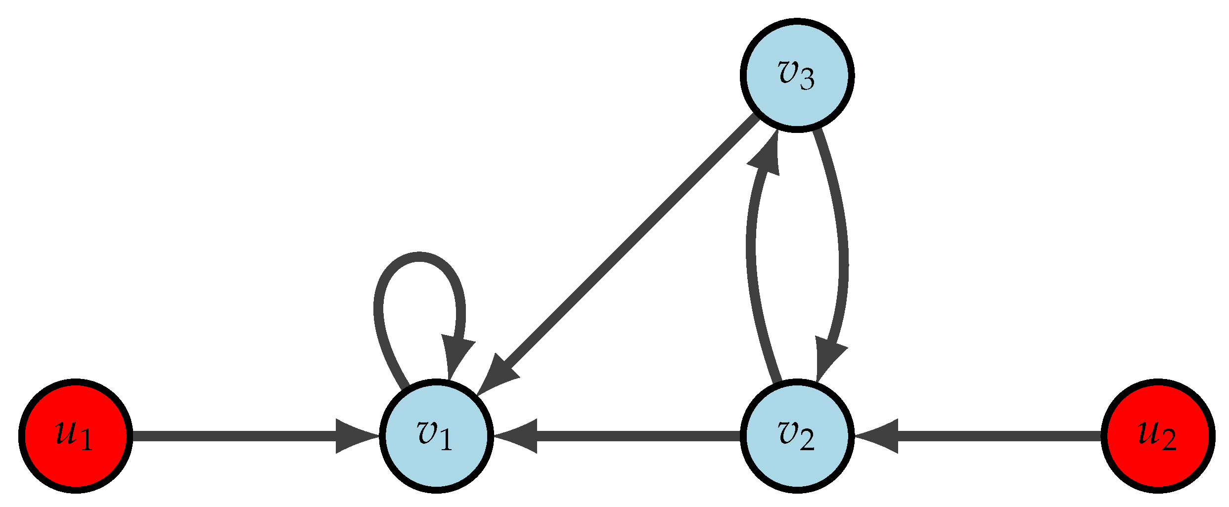
(i) 

Every node have external control input.

(ii) 

$\left(A_i+c_{ii}{H}_i,B_i\right)$ is controllable for all $i=1,2,\dots N$.

Proof. 

Suppose that the networked system (3) is controllable and suppose that $d_i=0$ for some i, say $i_0$, i.e., $d_{i_0}=0$. Then the control matrix for the networked system (3) is given by

$$G=\left[\begin{array}{cccccc}{d}_1{B}_1& 0& \dots & 0& \dots & 0\\ 0& d_2{B}_2& \dots & 0& \dots & 0\\ ⋮& ⋮& \ddots & ⋮& ⋮& ⋮\\ 0& 0& \dots & d_{i_0}{B}_{i_0}& \dots & 0\\ ⋮& ⋮& ⋮& ⋮& \ddots & ⋮\\ 0& 0& \dots & 0& \dots & d_N{B}_N\end{array}\right]=\left[\begin{array}{cccccc}{d}_1{B}_1& 0& \dots & 0& \dots & 0\\ 0& d_2{B}_2& \dots & 0& \dots & 0\\ ⋮& ⋮& \ddots & ⋮& ⋮& ⋮\\ 0& 0& \dots & 0& \dots & 0\\ ⋮& ⋮& ⋮& ⋮& \ddots & ⋮\\ 0& 0& \dots & 0& \dots & d_N{B}_N\end{array}\right]$$

We have proved that $e_{i_0}\otimes {\xi }_{i_{0}j}^k,k=1,2,\dots ,{\gamma }_{i_{0}j}$ are left eigenvectors of F corresponding to the eigenvalue ${\mu }_{i_0}^j$, where $j=1,2,\dots ,q_{i_0}$. Observe that for any $j=1,2,\dots ,q_{i_0},k=1,2,\dots ,{\gamma }_{i_{0}j}$, $\left(e_{i_0}\otimes {\xi }_{i_{0}j}^k\right)G=0$. Then, by Lemma 3, the given system is not controllable, which is a contradiction. Now, suppose that $\left(A_i+c_{ii}{H}_i,B_i\right)$ is not controllable for some i, say $i_1$. Again by Lemma 3, for some eigenvalue ${\mu }_{i_1}^{j_1}$ (where $j_1\in \{1,2,\dots ,q_{i_1}\}$) of $A_{i_1}+c_{i_1{i}_1}{H}_{i_1}$ there exists a left eigenvector ${\xi }_{i_1{j}_1}^{k_1}$ (where $k_1\in \{1,2,\dots ,{\gamma }_{i_1{j}_1}\}$), such that ${\xi }_{i_1{j}_1}^{k_1}{B}_{i_1}=0$. Then clearly $\left(e_{i_1}\otimes {\xi }_{i_1{j}_1}^{k_1}\right)G=0,$ which is a contradiction.

Conversely, suppose that both $\left(i\right)$ and $\left(ii\right)$ are satisfied. We have the left eigenvectors of F are $e_i\otimes {\xi }_{ij}^k$, where $i=1,2,\dots ,N,j=1,2,\dots ,q_i,k=1,2,\dots ,{\gamma }_{ij}$ or their linear combinations. Now $\left(e_i\otimes {\xi }_{ij}^k\right)G=0$ if, and only if, either $d_i=0,{\xi }_{ij}^k{B}_i=0$ or both for some i. Both of these situations contradict our hypothesis. Then by Lemma 3, system (3) is controllable. □

Example 4.

Consider a heterogeneous networked system with three nodes, where the state matrices and control matrices are given by

$$A_1=\left[\begin{array}{ccc}1& 2& 1\\ 1& 1& -1\\ 0& 1& 2\end{array}\right],A_2=\left[\begin{array}{ccc}1& 0& 0\\ -1& 1& 0\\ 0& -1& 1\end{array}\right],A_3=\left[\begin{array}{ccc}1& 1& -1\\ 0& 1& 0\\ 0& -1& 1\end{array}\right],B_1=\left[\begin{array}{c}1\\ 0\\ -1\end{array}\right],B_2=\left[\begin{array}{c}1\\ 1\\ -1\end{array}\right],B_3=\left[\begin{array}{c}0\\ 1\\ 1\end{array}\right]$$

The inner-coupling matrices are given by,

$$H_1=\left[\begin{array}{ccc}1& 1& -1\\ 0& 0& 0\\ 1& 1& -1\end{array}\right],H_2=\left[\begin{array}{ccc}0& 0& 0\\ 1& 2& 0\\ -1& 0& 1\end{array}\right],H_3=\left[\begin{array}{ccc}1& 0& 2\\ 0& 0& 0\\ 2& -1& 1\end{array}\right]$$

The left eigenvectors of $A_1$ are ${\xi }_{11}^1=\left[\begin{array}{ccc}-1& -1& 1\end{array}\right],{\xi }_{12}^1=\left[\begin{array}{ccc}-1& 1& 1\end{array}\right]$ and the only left eigenvector of $A_2$ is ${\xi }_{21}^1=\left[\begin{array}{ccc}1& 0& 0\end{array}\right]$. We have ${\xi }_{11}^1{H}_1={\xi }_{12}^1{H}_1={\xi }_{21}^1{H}_2=0$.

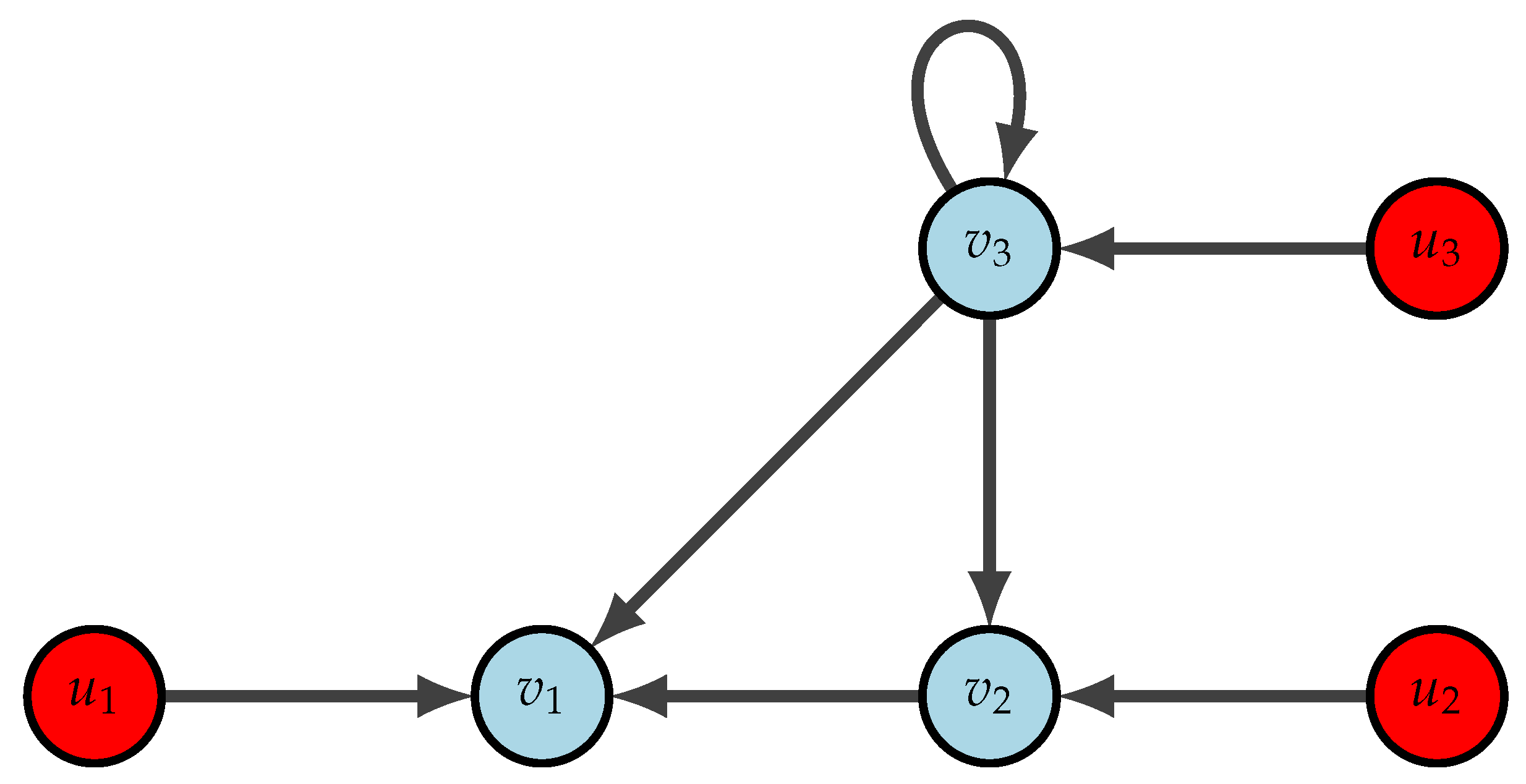
(i) 

From Figure 4, it is clear that all the nodes have external control input.

(ii) 

$(A_1,B_1),(A_2,B_2)$ and $(A_3+H_3,B_3)$ are controllable.

Thus, all the conditions of Theorem 5 are satisfied. Therefore, the given networked system is controllable.

5. Conclusions and Future Scope of Work

This paper provides a necessary and sufficient condition for the controllability of a heterogeneous networked system. Ajayakumar et al. [26] analyzed heterogeneous networked systems having identical control matrices in each node and obtained a necessary and sufficient conditions for controllability. Based on this work, it is possible to identify the nodes that required external control inputs in order to make the uncontrollable system controllable. In the present work, control matrices are considered to be distinct in each node and in addition to identifying the nodes that will receive control inputs, it is also possible to identify the control input matrices that needed to be employed. The existing results tell us less than ours about how subsystem dynamics, network topology, etc., affect the controllability of a networked system, and our results are easy to validate. In addition, controllability results for a more general class of heterogeneous networked systems over a particular network topology are obtained. We plan to look into the controllability of networked systems over more general network topologies in the future. The ability to control networked systems with delays and impulses could be another study area. However, research is performed in this direction for homogeneous networked systems with one-way communication and control delays, and this kind of study still needs to be performed on heterogeneous networked systems.

References

- Strogatz, S.H. Exploring complex networks. Nature 2001, 410, 268–276. [Google Scholar] [CrossRef] [PubMed] [Green Version]
- Wang, X.F.; Chen, G. Complex networks: Small-world, scale-free and beyond. IEEE Circuits Syst. Mag. 2003, 3, 6–20. [Google Scholar] [CrossRef] [Green Version]
- Xiang, L.; Chen, F.; Ren, W.; Chen, G. Advances in network controllability. IEEE Circuits Syst. Mag. 2019, 19, 8–32. [Google Scholar] [CrossRef]
- Kalman, R.E. On the general theory of control systems. IRE Trans. Autom. Control 1959, 4, 110. [Google Scholar] [CrossRef]
- Lin, C.T. Structural controllability. IEEE Trans. Autom. Control 1974, 19, 201–208. [Google Scholar]
- Hautus, M.L. Controllability and observability conditions of linear autonomous systems. Ned. Akad. Wet. 1969, 72, 443–448. [Google Scholar]
- Glover, K.; Silverman, L. Characterization of structural controllability. IEEE Trans. Autom. Control 1976, 21, 534–537. [Google Scholar] [CrossRef]
- Mayeda, H. On structural controllability theorem. IEEE Trans. Autom. Control 1981, 26, 795–798. [Google Scholar] [CrossRef]
- Tarokh, M. Measures for controllability, observability and fixed modes. IEEE Trans. Autom. Control 1992, 37, 1268–1273. [Google Scholar] [CrossRef]
- Tanner, H.G. On the controllability of nearest neighbor interconnections. In Proceedings of the 2004 43rd IEEE Conference on Decision and Control (CDC) (IEEE Cat. No. 04CH37601), Nassau, Bahamas, 14–17 December 2004; Volume 3, pp. 2467–2472. [Google Scholar]
- Rahmani, A.; Mesbahi, M. Pulling the strings on agreement: Anchoring, controllability, and graph automorphisms. In Proceedings of the 2007 American Control Conference, New York, NY, USA, 9–11 July 2007; pp. 2738–2743. [Google Scholar]
- Liu, X.; Lin, H.; Chen, B.M. Graph-theoretic characterisations of structural controllability for multi-agent system with switching topology. Int. J. Control 2013, 86, 222–231. [Google Scholar] [CrossRef]
- Yazıcıoğlu, A.Y.; Abbas, W.; Egerstedt, M. Graph distances and controllability of networks. IEEE Trans. Autom. Control 2016, 61, 4125–4130. [Google Scholar] [CrossRef] [Green Version]
- Farhangi, H. The path of the smart grid. IEEE Power Energy Mag. 2009, 8, 18–28. [Google Scholar] [CrossRef]
- Wuchty, S. Controllability in protein interaction networks. Proc. Natl. Acad. Sci. USA 2014, 111, 7156–7160. [Google Scholar] [CrossRef] [PubMed] [Green Version]
- Gu, S.; Pasqualetti, F.; Cieslak, M.; Telesford, Q.K.; Alfred, B.Y.; Kahn, A.E.; Medaglia, J.D.; Vettel, J.M.; Miller, M.B.; Grafton, S.T.; et al. Controllability of structural brain networks. IEEE Nat. Commun. 2015, 6, 1–10. [Google Scholar] [CrossRef] [Green Version]
- Bassett, D.S.; Sporns, O. Network neuroscience. Nat. Neurosci. 2017, 20, 353–364. [Google Scholar] [CrossRef] [Green Version]
- Zhou, T. On the controllability and observability of networked dynamic systems. Automatica 2015, 52, 63–75. [Google Scholar] [CrossRef] [Green Version]
- Wang, L.; Chen, G.; Wang, X.; Tang, W.K. Controllability of networked MIMO systems. Automatica 2016, 69, 405–409. [Google Scholar] [CrossRef] [Green Version]
- Wang, L.; Wang, X.; Chen, G. Controllability of networked higher-dimensional systems with one-dimensional communication. In Philosophical Transactions of the Royal Society A: Mathematical, Physical and Engineering Sciences; Royal Society: London, UK, 2017; Volume 375, p. 20160215. [Google Scholar]
- Hao, Y.; Duan, Z.; Chen, G. Further on the controllability of networked MIMO LTI systems. Int. J. Robust Nonlinear Control 2018, 28, 1778–1788. [Google Scholar] [CrossRef]
- Wang, P.; Xiang, L.; Chen, F. Controllability of heterogeneous networked MIMO systems. In Proceedings of the 2017 International Workshop on Complex Systems and Networks (IWCSN), Doha, Qatar, 8–10 December 2017; pp. 45–49. [Google Scholar]
- Xiang, L.; Wang, P.; Chen, F.; Chen, G. Controllability of directed networked MIMO systems with heterogeneous dynamics. IEEE Trans. Control Netw. Syst. 2019, 7, 807–817. [Google Scholar] [CrossRef]
- Ajayakumar, A.; George, R.K. A Note on Controllability of Directed Networked System with Heterogeneous Dynamics. IEEE Trans. Control Netw. Syst. 2022, 2022, 1–4. [Google Scholar] [CrossRef]
- Kong, Z.; Cao, L.; Wang, L.; Guo, G. Controllability of Heterogeneous Networked Systems with Non-identical Inner-coupling Matrices. IEEE Trans. Control Netw. Syst. 2022, 9, 867–878. [Google Scholar] [CrossRef]
- Ajayakumar, A.; George, R.K. Controllability of networked systems with heterogeneous dynamics. Math. Control Signals Syst. 2023, 1–20. [Google Scholar] [CrossRef]
- Horn, R.A.; Johnson, C.R. Topics in Matrix Analysis; Cambridge University Press: Cambridge, UK, 1994. [Google Scholar]
- Horn, R.A.; Johnson, C.R. Matrix Analysis; Cambridge University Press: Cambridge, UK, 2012. [Google Scholar]
- Rugh, W.J. Linear System Theory; Prentice-Hall, Inc.: Kalamazoo, MI, USA, 1996. [Google Scholar]
Disclaimer/Publisher’s Note: The statements, opinions and data contained in all publications are solely those of the individual author(s) and contributor(s) and not of MDPI and/or the editor(s). MDPI and/or the editor(s) disclaim responsibility for any injury to people or property resulting from any ideas, methods, instructions or products referred to in the content. |
© 2023 by the authors. Licensee MDPI, Basel, Switzerland. This article is an open access article distributed under the terms and conditions of the Creative Commons Attribution (CC BY) license (https://creativecommons.org/licenses/by/4.0/).
Share and Cite
Ajayakumar, A.; George, R.K. Controllability of a Class of Heterogeneous Networked Systems. Foundations 2023, 3, 167-180. https://doi.org/10.3390/foundations3020015
Ajayakumar A, George RK. Controllability of a Class of Heterogeneous Networked Systems. Foundations. 2023; 3(2):167-180. https://doi.org/10.3390/foundations3020015
Chicago/Turabian StyleAjayakumar, Abhijith, and Raju K. George. 2023. "Controllability of a Class of Heterogeneous Networked Systems" Foundations 3, no. 2: 167-180. https://doi.org/10.3390/foundations3020015