Zero-Energy Bound States of Neutron–Neutron or Neutron–Muon Systems

Abstract

There exists the following paradigm: for interaction potentials U(r) that are negative and go to zero as r goes to infinity, bound states may exist only for the negative total energy E. For E > 0 and for E = 0, bound states are considered to be impossible, both in classical and quantum mechanics. In the present paper we break this paradigm. Namely, we demonstrate the existence of bound states of E = 0 in neutron–neutron systems and in neutron–muon systems, specifically when the magnetic moments of the two particles in the pair are parallel to each other. As particular examples, we calculate the root-mean-square size of the bound states of these systems for the values of the lowest admissible values of the angular momentum, and show that it exceeds the neutron radius by an order of magnitude. We also estimate the average kinetic energy and demonstrate that it is nonrelativistic. The corresponding bound states of E = 0 may be called “neutronium” (for the neutron–neutron systems) and “neutron–muonic atoms” (for the neutron–muon systems). We also point out that this physical system possesses higher-than-geometric (i.e., algebraic) symmetry, leading to the approximate conservation of the square of the angular momentum, despite the geometric symmetry being axial. We use this fact for facilitating analytical and numerical calculations.

1. Introduction

There exists the following paradigm: for interaction potentials U(r) that are negative and go to zero as r goes to infinity, bound states may exist only for the negative total energy E. For E > 0 and for E = 0, bound states are considered to be impossible, both in classical and quantum mechanics. For example, in sect. 18 of the textbook [1], it was stated that for potentials falling off at large r as −1/r^s with s > 2 (which is the case for the potential analyzed in the present paper), the highest discrete energy level has some nonzero negative value E_max, so that states of E > E_max, including E = 0, cannot correspond to the bound states.

In the present paper we break this paradigm. Namely, we demonstrate the existence of bound states of E = 0 in neutron–muon systems and in neutron–neutron systems, specifically when the magnetic moments of the two particles in the pair are parallel to each other. It should be emphasized that we describe the bound states where the energy is exactly zero, not the bound states of the infinitesimal negative energy.

The aligned magnetic moments define the preferred direction in space. So, the geometrical symmetry of the system is axial, leading to the conservation of the angular momentum projection on the axis. However, we point out that the system has a higher-than-geometrical (i.e., algebraic) symmetry, leading to the (approximate) conservation of the square of the angular momentum as well. We employ this fact for finding a zero-total-energy solution for the wave function. The wave function turns out to correspond to the bound state of E = 0. The corresponding bound state may be called “neutron–muonic atom” (for the neutron–muon system) and “neutronium” (for the neutron–neutron systems).

We calculate the root-mean-square separation between the neutron and muon, as well as between the neutron and neutron, and show that it significantly exceeds the neutron radius. We also estimate the average kinetic energy and demonstrate that it is nonrelativistic.

2. Analysis

We start by consider a system of two-spin 1/2 particles (1 and 2), having parallel magnetic moments μ₁ and μ₂, respectively. Particle 1 is electrically neutral (e.g., the neutron). Particle 2 is either charged (e.g., the muon) or electrically neutral (e.g., the neutron).

We focus on the situation where the orbital momentum projection L_z = 0, the z-axis being chosen along the common direction of the magnetic moments μ₁ and μ₂. Then the spin–orbit interaction, being proportional to the scalar product of the operators S and L (where S is the total spin) vanishes.

For the zero-total-energy states, the kinetic energy K should be equal by magnitude and opposite by the sign of the potential energy U. In the spherical polar coordinates, the potential energy is (see textbook [2], sect. 44).

U(r, cos θ) = μ₁μ₂(1 − 3 cos²θ)/r³ = μ₁μ₂(1 − 3 cos²θ)/r³,

(1)

where θ is the polar angle of the radius-vector r and μ₁μ₂ is the scalar product (also known as the dot-product) of these two vectors.

Physical systems described by the potential from Equation (1) have the following remarkable feature. They have the algebraic symmetry higher than the geometrical symmetry. While the geometrical symmetry is axial (leading to the conservation of the L_z component of the angular momentum), there is the (approximate) spherical symmetry, leading to the (approximate) conservation of the square of the angular momentum. This property of such potentials was noted and employed in celestial mechanics, e.g., while describing the motion of a satellite about the oblate Earth ([3], sect. 1.7), the motion of a circumbinary planet [4], and the motion of an interstellar interloper passing a circular binary star [5]. It was also noted and used in atomic physics while analyzing a hydrogen atom under a high-frequency, linearly polarized laser field [6,7].

For the above reason, L can be considered as a good quantum number, so that the angular part of the wave function can be described by the spherical harmonics. Thus, in the Schrödinger equation for E = 0,

[K + U(r, cos θ)] ψ (r, θ) = 0,

(2)

it is legitimate to represent:

ψ (r, θ) = R_0L(r) Y_L0(θ).

(3)

In Equation (3), Y_L0(θ) is the spherical harmonic (corresponding to L_z = 0) and R_0L(r) is the radial part of the wave function (its subscript 0 indicates that it corresponds to E = 0).

For simplifying the treatment of the problem to allow obtaining analytical results, at least approximately, we average U(r, cos θ) from Equation (3) over the corresponding spherical harmonic:

$${\mathrm{U}}_{\mathrm{L}}\left(\mathrm{r}\right)=4\mathrm{\pi } {\displaystyle \underset{0}{\overset{1}{\int }}} \mathrm{d}(\cos \mathsf{\theta }) {\left[{\mathrm{Y}}_{\mathrm{L}0}\right(\mathsf{\theta }\left)\right]}^2 \mathrm{U}(\mathrm{r}, \cos \mathsf{\theta }).$$

(4)

For example, for L = 2, L = 3, and L = 4, Equation (4) yields:

U₂(r) = −(4/7) μ₁μ₂₀/r³,

(5)

U₃(r) = −(8/15) μ₁μ₂₀/r³.

(6)

U₄(r) = −(40/99) μ₁μ₂₀/r³,

(7)

It is seen that U_L(r) is the attractive potential of the form.

U_L(r) = −g(L) μ₁μ₂/r³,

(8)

where g(2) = 4/7, g(3) = 8/15, and g(4) = 40/99.

Now, the Schrödinger equation for E = 0 can be represented in the form:

[p²/(2m_red) − g(L) μ₁μ₂/r³]ψ = 0,

(9)

where p is the operator of the linear momentum and m_red is the reduced mass of the pair of the particles.

m_red = m₁m₂/(m₁ + m₂),

(10)

m₁ and m₂ being the masses of particles 1 and 2, respectively.

Equation (9) can be rewritten as follows:

[ħ²/(2m_redr²)] [−r²(d²R/dr²) − 2r(dR/dr) + L(L + 1)R] − [g(L) μ₁μ₂/r³] R = 0,

(11)

or equivalently:

d²R/dr² + (2/r) (dR/dr) − L(L + 1)R/r² +2g(L)m_redμ₁μ₂R/(ħ²r³) = 0.

(12)

After the standard substitution:

R(r) = χ(r)/r,

(13)

Equation (12) takes the form:

d²χ/dr² − [L(L + 1)/r²]χ + B/r³ = 0,

(14)

where

B = 2g(L)m_redμ₁μ₂χ/(ħ²).

(15)

Now we study the behavior of the solution χ(r) at small and large r. At a relatively small r, Equation (14) can be simplified to

d²χ/dr² ≈ −Bχ/r³.

(16)

We seek the solution of Equation (14) in the form:

χ(r) = const cos(a/r^b).

(17)

On substituting Equation (17) in Equation (16), we get

−[ab(b + 1)/r^b+2] sin(a/r^b) − [a²b²/r^2b+2]χ ≈ − (a²b²/r^2b+2)χ ≈ −(B/r³)χ.

(18)

In Equation (18), while proceeding from the utmost left part to the middle part, we omitted the first term since at small r the second term dominates. From Equation (18) it follows that

b = 1/2, a = 2B^1/2,

(19)

so that for a relatively small r, we have

χ(r) ≈ const cos(2B^1/2/r^1/2).

(20)

At a relatively large r, Equation (14) can be simplified to

d²χ/dr² ≈ [L(L + 1)/r²]χ.

(21)

We seek the solution of Equation (21) in the form:

χ(r) = const/r^q.

(22)

On substituting Equation (22) in Equation (21), we get

q(q + 1)/r^q+2 ≈ [L(L + 1)/r^q+2.

(23)

From Equation (23) it follows that

q = L

(24)

(the second possible value q = −L − 1 is physically inadmissible).

So, at a relatively large r, the solution of Equation (14) is

χ(r) ≈ const/r^L.

(25)

In view of the two asymptotics, given by Equations (20) and (25), it is easy to see that the normalization integral

$$\underset{0}{\overset{\infty }{\int }}\mathrm{d}\mathrm{r} {\left[\mathrm{\chi }\right(\mathrm{r}\left)\right]}^2 = 1$$

(26)

converges for any L ≥ 1 (though the average value of r and the root-mean-square value of r_rms exist only for L ≥ 2).

Thus, in some systems of the two particles, coupled only by the interaction of two magnetic dipoles, there can exist bound states of the zero total energy. This result amounts to breaking the paradigm that such bound states are impossible.

The availability of the analytical expressions for χ(r) at small r and at large r simplifies obtaining numerical solutions of Equation (14) for various values of L. Below we provide some examples.

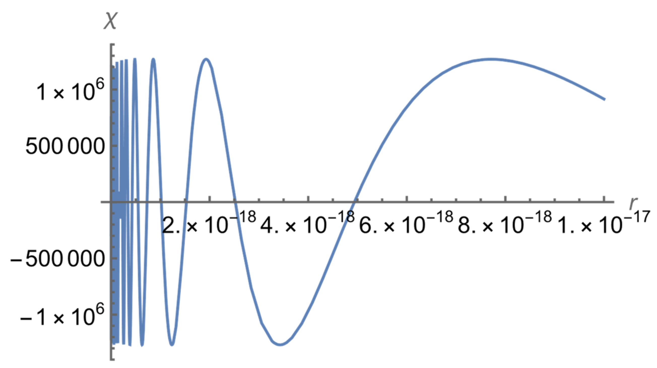
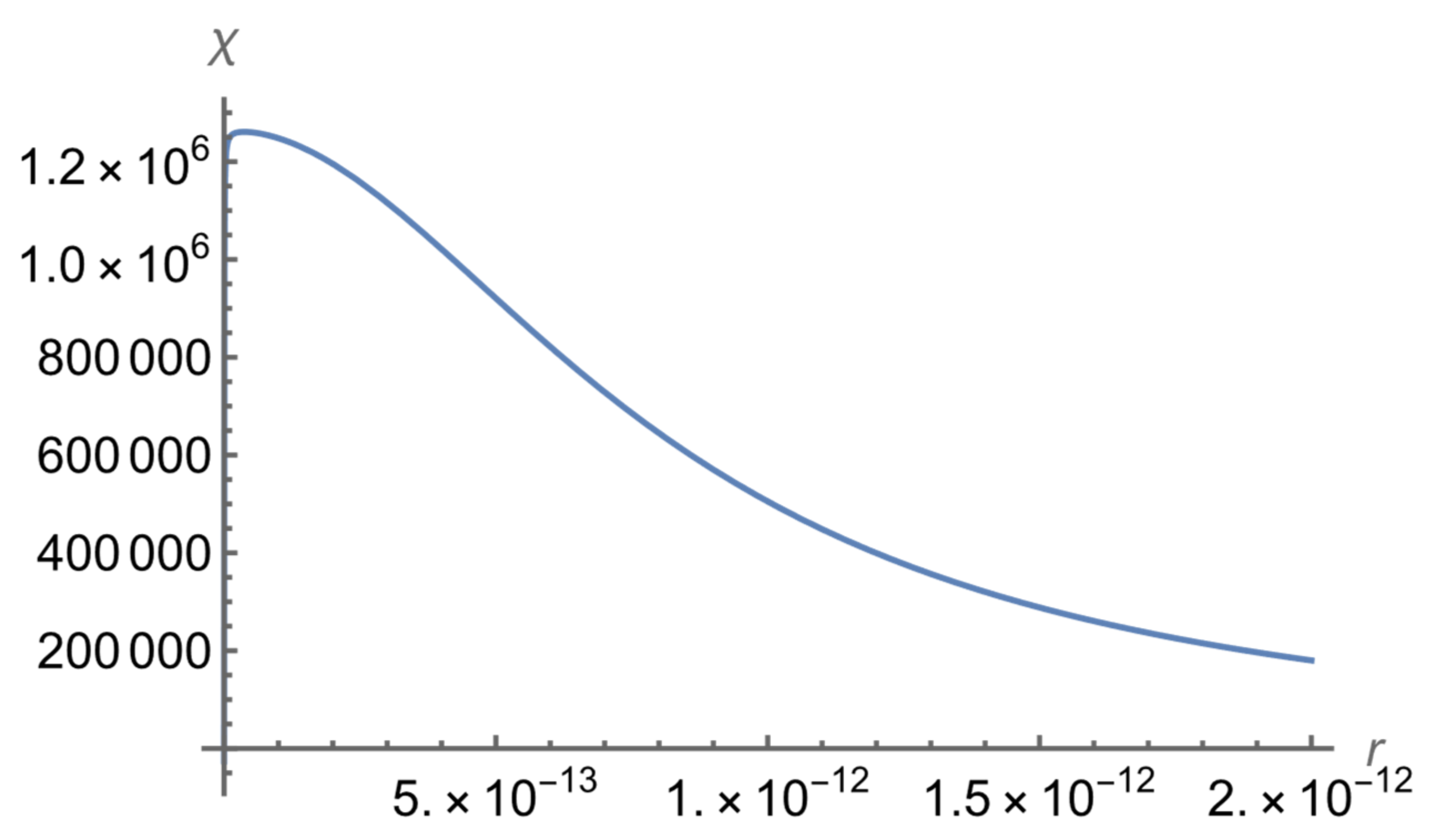
The first example is a neutron–muon system in the state of L = 2 and where the magnetic moments of the two particles are parallel (so that the spins are parallel). Our calculation shows that there exists a bound state (of E = 0) having r_rms = 8.3 × 10⁻¹³ cm, which exceeds the neutron radius by an order of magnitude. We also estimate the average kinetic energy <K>—to make sure that the values of <K> do not contradict the nonrelativistic treatment of this physical system. (Here and below, the symbol <…> means the “average value”). Specifically, we estimate K by using the uncertainty relation p ~ ħ/(2r), so that

K ~ [ħ²/(8m_red)] <1/r²>,

(27)

where

$$<1/{\mathrm{r}}^2>=\underset{{\mathrm{r}}_{\mathrm{n}}}{\overset{\infty }{\int }} \mathrm{d}\mathrm{r} {\left[\mathrm{\chi }\right(\mathrm{r}\left)\right]}^2/{\mathrm{r}}^2.$$

(28)

At small r, we truncated the integration in Equation (28) at the neutron radius r_n = 0.87 × 10⁻¹³ cm for avoiding the divergence of the integral at small r. The estimated average kinetic energy is <K>~8.6 Mev, so that the nonrelativistic treatment is justified since the rest energy of the muon is about 106 Mev.

Below are the plots of the corresponding normalized wave function at a relatively small r (Figure 1) and at a relatively large r (Figure 2).

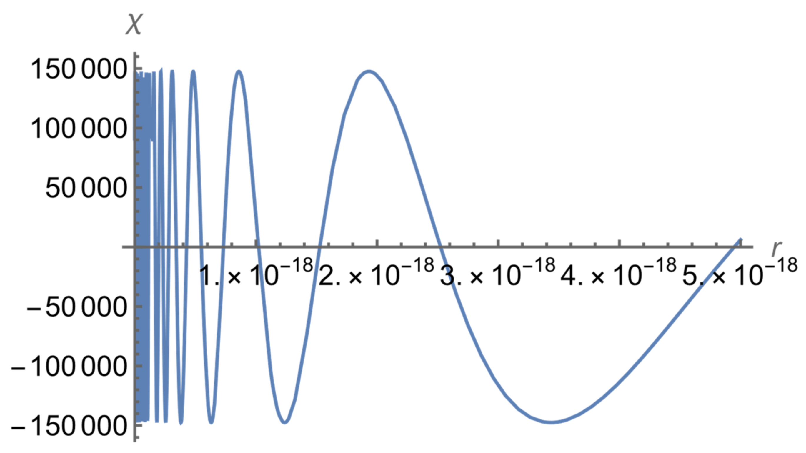
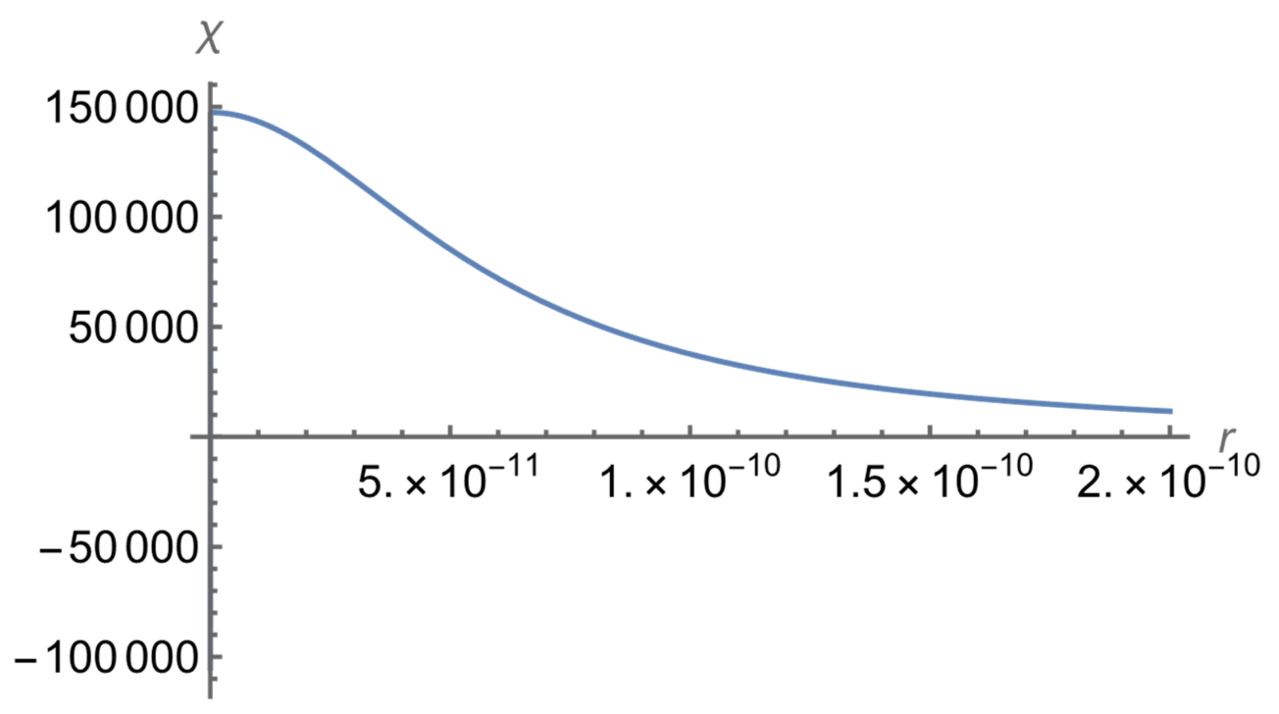
The second example is a neutron–neutron system. This system is invariant with respect to the inversion of the reference frame, so that the states of the system have a definite parity P = (−1)^L (see the textbook [1]). Since the two particles are identical, in the state of the parallel spins, and thus parallel magnetic moment (which is the state we are interested in), the coordinate wave function must be antisymmetric (see the textbook [1]), so that the parity P = −1. Therefore, only the states of odd values of L are admissible. Together with the above restriction L ≥ 2, this means that the lowest admissible value of the angular momentum for this system is L = 3.

So, with respect to the quantum number L, the situation for the neutron–neutron systems is a little bit more restrictive than for the neutron–muon systems. However, in terms of the projection L_z, the situation for the neutron–neutron systems is significantly less restrictive than for the neutron–muon systems. Indeed, for the latter systems, we required L_z = 0 to “kill” the spin–orbit interaction. For the neutron–neutron systems, there is no such restriction because for these systems the spin–orbit interaction does not exist.

Our calculation shows that for L = 3, there exists a bound state (of E = 0) having r_rms = 7.2 × 10⁻¹³ cm, which exceeds the neutron radius by an order of magnitude. The average kinetic energy in this state is estimated as <K>~1.6 MeV, so that the nonrelativistic treatment is justified since the rest energy of the neutron is about 939 Mev.

Below are the plots of the corresponding normalized wave function at a relatively small r (Figure 3) and at a relatively large r (Figure 4).

3. Conclusions

We studied the systems of the two particles, coupled only by the interaction of two magnetic dipoles. We demonstrated that in such systems there can exist bound states of the zero total energy. Thus, we broke the paradigm that bound states of the zero total energy are impossible. This general result, related to the foundations of quantum mechanics, is of fundamental importance.

As particular examples, we studied the neutron–muon systems and the neutron–neutron systems. We calculated the root-mean-square size of the bound states of these systems for the lowest admissible values of the angular momentum: L = 2 for the neutron–muon systems, and L = 3 for the neutron–neutron systems. We also provided estimates of the corresponding average values of the kinetic energy and showed that the obtained values do not contradict to the nonrelativistic treatment of the problem under consideration. The corresponding bound states may be called “neutron–muonic atoms” and “neutronium” for the second example.

Another fundamental importance of our findings seems to be in revealing a new physical system possessing higher-than-geometric symmetry. The resulting approximate conservation of the square of the angular momentum (despite the geometric symmetry only being axial) is the common feature this physical system shares with a satellite around an oblate planet, or a circumbinary planet, or an interstellar interloper passing a circular binary star, or a hydrogen atom under the high-frequency, linearly polarized laser field.

For completeness, we note that there are many studies of systems where there is the interaction of an electric (rather than magnetic) dipole with a charged particle (see papers [8,9,10] and references therein). However, the physics of these systems differs from the one considered in the present paper.

References

- Landau, L.D.; Lifshitz, E.M. Quantum Mechanics; Pergamon: Oxford, UK, 1965. [Google Scholar]
- Landau, L.D.; Lifshitz, E.M. The Classical Theory of Fields; Pergamon: Oxford, UK, 1962. [Google Scholar]
- Beletsky, V.V. Essays on the Motion of Celestial Bodies; Birkhäuser/Springer: Basel, Switzerland, 2001. [Google Scholar]
- Oks, E. Analytical Solution for the Three-Dimensional Motion of a Circumbinary Planet Around a Binary Star. New Astron. 2020, 74, 101301. [Google Scholar] [CrossRef]
- Oks, E. Circular Binary Star and an Interstellar Interloper: The Analytical Solution. New Astron. 2021, 84, 101500. [Google Scholar] [CrossRef]
- Gavrilenko, V.P.; Oks, E.; Radchik, A.V. Hydrogen-Like Atom in a Field of High-Frequency Linearly-Polarized Electromagnetic Radiation. Opt. Spectrosc. 1985, 59, 411–412. [Google Scholar]
- Nadezhdin, B.B.; Oks, E. Highly Excited Atom in a High-Frequency Field of Linearly-Polarized Electromagentic Radiation. Sov. Tech. Phys. Lett. 1986, 12, 512–513. [Google Scholar]
- Baryshnikov, F.F.; Zakharov, L.E.; Lisitsa, V.S. Electron Bremsstrahlung in a Dipole Potential. Sov. Phys. JETP 1980, 52, 406–411. [Google Scholar]
- Sanders, P.; Oks, E. Allowance for More Realistic Trajectories of Plasma Electrons in the Stark Broadening of Hydrogenlike Spectral Lines. J. Phys. Commun. 2018, 2, 035033. [Google Scholar] [CrossRef]
- Oks, E. Oscillatory-Precessional Motion of a Rydberg Electron Around a Polar Molecule. Symmetry 2020, 12, 1275. [Google Scholar] [CrossRef]
Figure 1.
The normalized wave function of the bound E = 0 state of the neutron–muon system for L = 2 at a relatively small r.
Figure 2.
The normalized wave function of the bound E = 0 state of the neutron–muon system for L = 2 at a relatively large r.
Figure 3.
The normalized wave function of the bound E = 0 state of the neutron–neutron system for L = 3 at a relatively small r.
Figure 4.
The normalized wave function of the bound E = 0 state of the neutron–neutron system for L = 3 at a relatively large r.
Disclaimer/Publisher’s Note: The statements, opinions and data contained in all publications are solely those of the individual author(s) and contributor(s) and not of MDPI and/or the editor(s). MDPI and/or the editor(s) disclaim responsibility for any injury to people or property resulting from any ideas, methods, instructions or products referred to in the content. |
© 2023 by the author. Licensee MDPI, Basel, Switzerland. This article is an open access article distributed under the terms and conditions of the Creative Commons Attribution (CC BY) license (https://creativecommons.org/licenses/by/4.0/).
Share and Cite
MDPI and ACS Style
Oks, E. Zero-Energy Bound States of Neutron–Neutron or Neutron–Muon Systems. Foundations 2023, 3, 65-71. https://doi.org/10.3390/foundations3010007
AMA Style
Oks E. Zero-Energy Bound States of Neutron–Neutron or Neutron–Muon Systems. Foundations. 2023; 3(1):65-71. https://doi.org/10.3390/foundations3010007
Chicago/Turabian StyleOks, Eugene. 2023. "Zero-Energy Bound States of Neutron–Neutron or Neutron–Muon Systems" Foundations 3, no. 1: 65-71. https://doi.org/10.3390/foundations3010007