Article

Extended Convergence of Two Multi-Step Iterative Methods

1
Department of Mathematics, University of Houston, Houston, TX 77204, USA
2
Department of Computing and Mathematical Sciences, Cameron University, Lawton, OK 73505, USA
3
Department of Mathematics, Puducherry Technological University, Pondicherry 605014, India
*
Author to whom correspondence should be addressed.
Foundations 2023, 3(1), 140-153; https://doi.org/10.3390/foundations3010013
Submission received: 21 February 2023 / Revised: 9 March 2023 / Accepted: 10 March 2023 / Published: 13 March 2023

Abstract

:
Iterative methods which have high convergence order are crucial in computational mathematics since the iterates produce sequences converging to the root of a non-linear equation. A plethora of applications in chemistry and physics require the solution of non-linear equations in abstract spaces iteratively. The derivation of the order of the iterative methods requires expansions using Taylor series formula and higher-order derivatives not present in the method. Thus, these results cannot prove the convergence of the iterative method in these cases when such higher-order derivatives are non-existent. However, these methods may still converge. Our motivation originates from the need to handle these problems. No error estimates are given that are controlled by constants. The process introduced in this paper discusses both the local and the semi-local convergence analysis of two step fifth and multi-step 5 + 3 r order iterative methods obtained using only information from the operators on these methods. Finally, the novelty of our process relates to the fact that the convergence conditions depend only on the functions and operators which are present in the methods. Thus, the applicability is extended to these methods. Numerical applications complement the theory.

1. Introduction

The most commonly recurring problems in engineering, the physical and chemical sciences, computing and applied mathematics can be usually summed up as solving a non-linear equation of the form
G ( x ) = 0 ,
with G : D E 1 E 2 being differentiable as, per Fréchet, E 1 , E 2 denotes complete normed linear spaces and D is a non-empty, open and convex set.
Researchers have attempted for decades to trounce this nonlinearity. From the analytical view, these equations are very challenging to solve. The utilisation of iterative methods (IM) to find the solution of such non-linear equations is predominantly chosen among researchers for this very reason. The most predominantly used IM for solving such nonlinear equations is Newton’s method. In recent years, with advancements in science and mathematics, many new higher-order iterative methods for dealing with nonlinear equations have been found and are presently being employed [1,2,3,4,5,6,7,8]. Nevertheless, these results on the convergence of iterative methods that are currently being utilised in the above-mentioned articles are derived by applying high-order derivatives. In addition, no results address the error bounds, convergence radii or the domain in which the solution is unique.
The study of local convergence analysis (LCA) and semi-local analysis (SLA) of an IM permits calculating the radii of the convergence domains, error bounds and a region in which the solution is unique. The work in [9,10,11,12] discusses the results of local and semi-local convergence of different iterative methods. In the above-mentioned articles, important results discussing radii of convergence domains and measurements on error estimates are discussed, thereby expanding the utility of these iterative methods. Outcomes of these type of studies are crucial as they exhibit the difficulty in selecting starting points.
In this article, we establish theorems of convergence for two multi-step IMs with fifth (2) and 5 + 3 p (3) order convergence proposed in [8]. The methods are:
y i = x i G ( x i ) 1 G ( x i ) τ 1 ( x i ) = P i + 1 4 ( P i I ) 2 , P i = G ( y i ) 1 G ( x i ) x i + 1 = y i τ 1 ( x i ) G ( x i ) 1 G ( y i )
and
z 0 ( x i ) = x i G ( x i ) 1 G ( x i ) , z 1 ( x i ) = z 0 ( x i ) τ 1 ( x i ) G ( x i ) 1 G ( z 0 ( x i ) ) z 2 ( x i ) = z 1 ( x i ) τ 1 ( x i ) G ( x i ) 1 G ( z 1 ( x i ) ) x i + 1 = z p ( x i ) = z p 1 ( x i ) τ 1 ( x i ) G ( x i ) 1 G ( z p 1 ( x i ) ) ,
where p is a positive integer.
It is worth emphasizing that (2) and (3) are iterative and not analytical methods. That is, a solution denoted by x * is obtained as an approximation using these methods. The iterative methods are more popular than the analytical methods, since in general it is rarely possible to find the closed form of the solution in the latter form.
Motivation: The LCA of the methods (2) and (3) is given in [8]. The order is specified using Taylor’s formula and requires the employment of higher-order derivatives not present in the method. Additionally, these works cannot give estimates on the error bounds x i x * 
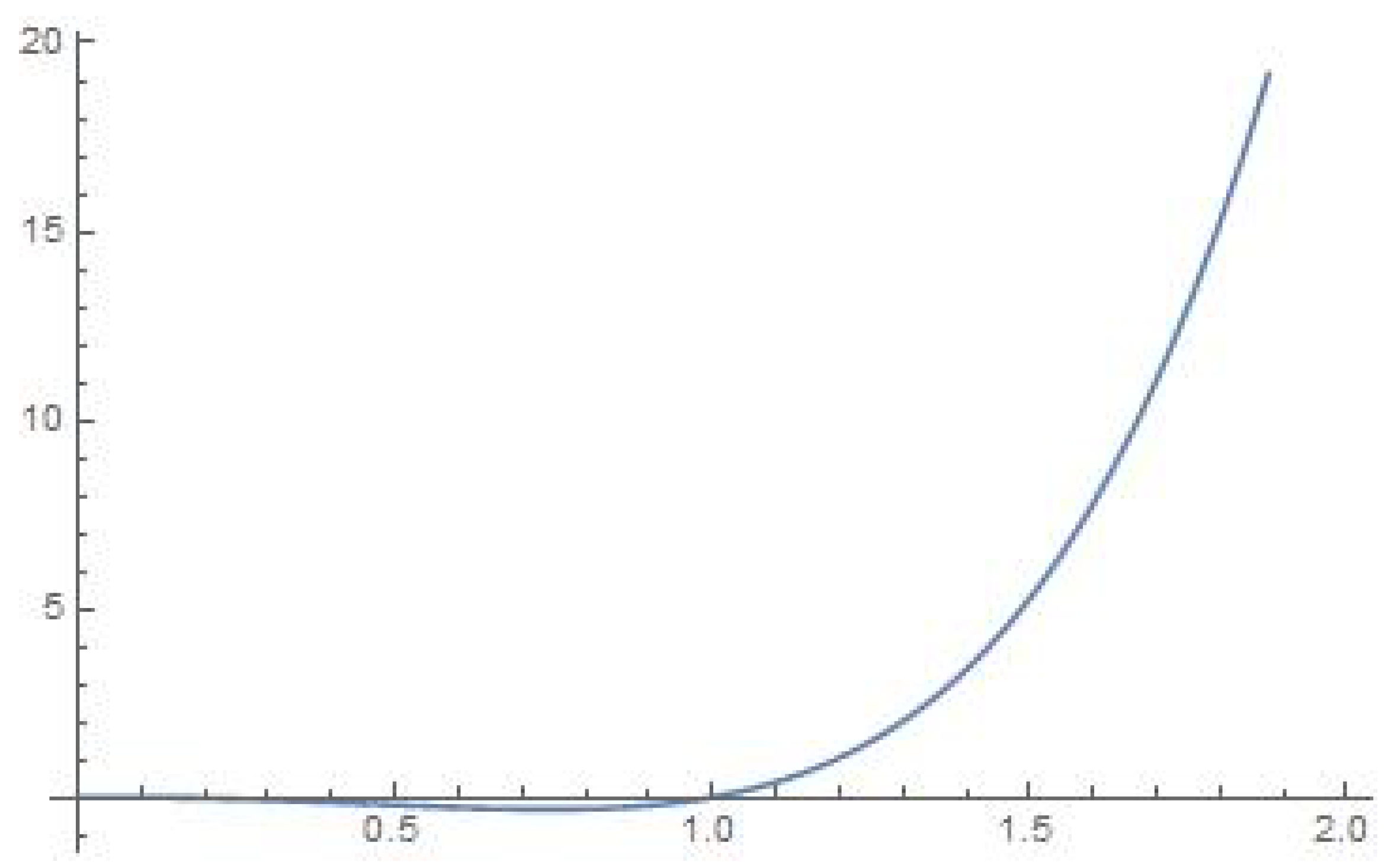
, the radii of convergence domains or the uniqueness domain. To observe the limitations of the Taylor series approach, consider G on D = [ 0.5 , 1.5 ] by
G ( t ) = t 3 ln ( t 2 ) + t 5 t 4 , if t 0 0 , if t = 0 .
Then, we can effortlessly observe that since G is unbounded, the conclusions on convergence of (2) and (3) discussed in [8] are not appropriate for this example.
Novelty: The aforementioned disadvantages provide encourage us to introduce convergence theorems providing the domains and hence comparing the domains of convergence of (2) and (3) by considering hypotheses based only on G . This research work also presents important results for the estimation of the error bounds x i x * and radii of the domain of convergence. Discussions about the exact location and the uniqueness of the root x * are also provided in this work.
The rest of the details of this article can be outlined as follows: Section 2 deals with LCA of the methods (2) and (3). The SLA considered more important than LC and not provided in [8] is also dealt with in this article in 
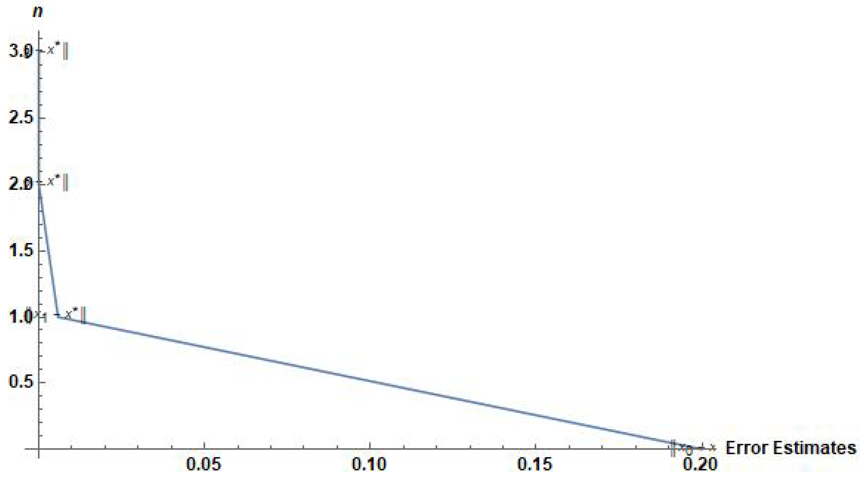
Section 3. The convergence outcomes are tested using numerical examples and are given in Section 4. Example 4 deals with a real world application problem. In Example 5, we revisit the motivational example to show that lim n + x n = x * = 1 . Conclusions of this study are given in Section 5.

2. Local Convergence Analysis

Some scalar functions are developed to prove the convergence. Let T = 0 , + .
Suppose:
(i)
There exists a function φ 0 : T R which is non-decreasing and continuous (NC) and the equation φ 0 ( t ) 1 = 0 admits a minimal solution (MS) ρ 0 T { 0 } . Set T 0 = 0 , ρ 0 .
(ii)
There exists a function φ : T 0 R which is NC so that the equation g 0 ( t ) 1 = 0 admits a MS r 0 T 0 { 0 } , with the function g 0 : T 0 R being
g 0 ( t ) = 0 1 φ ( ( 1 θ ) t ) d θ 1 φ 0 ( t ) .
(iii)
The equation φ 0 ( g 0 ( t ) t ) 1 = 0 admits a MS ρ T 0 { 0 } . Set T 1 = 0 , ρ 1 , where ρ 1 = m i n { ρ 0 , ρ } .
(iv)
The equation g 1 ( t ) 1 = 0 admits a MS r 1 T 1 { 0 } , provided the function g 1 : T 1 R is defined by
g 1 ( t ) = 0 1 φ ( ( 1 θ ) g 0 ( t ) t ) d θ 1 φ 0 ( g 0 ( t ) t ) + 1 4 ( φ ¯ ( t ) 1 φ 0 ( g 0 ( t ) t ) ) 2 ( 1 + 0 1 φ 0 ( θ g 0 ( t ) t ) d θ ) 1 φ 0 ( t ) g 0 ( t ) ,
where
φ ¯ ( t ) = φ ( ( 1 + g 0 ( t ) ) t ) , or φ 0 ( t ) + φ 0 ( g 0 ( t ) t ) .
In applications, the smallest version of the function φ ¯ shall be chosen.
Set
r = m i n { r 0 , r 1 } .
The parameter r is the radius of the convergence ball (RC) for the method (2) (see Theorem 1).
Set T 2 = 0 , r .
Then, if t T 2 , it is implied that
0 φ 0 ( t ) < 1 ,
0 φ 0 ( g 0 ( t ) t ) < 1 ,
0 g 0 ( t ) < 1
and 0 g 1 ( t ) < 1 .
The following conditions justify the introduction of the functions φ 0 and φ and helps in proving the LC of the method (2).
( A 1 )
There exists x * D with G ( x * ) = 0 and G ( x * ) 1 L ( E 2 , E 1 ) .
( A 2 )
G ( x * ) 1 ( G ( u ) G ( x * ) ) φ 0 ( u x * ) for each u D . Set D 0 = D S ( x * , ρ 0 ) .
( A 3 )
G ( x * ) 1 ( G ( u 2 ) G ( u 1 ) ) φ ( u 2 u 1 ) for each u 1 , u 2 D 0 .
and
( A 4 )
S [ x * , r ] D , with r given in (6).
Conditions ( A 1 )–( A 4 ) are employed to show the LC of the method (2). Let d i = x i x * .
Theorem 1.
Under the conditions ( A 1 )–( A 4 ), further assume that the starting point x 0 S ( x * , r ) { x * } . Then, the sequence { x i } given by the method (2) is convergent to x * and
y i x * g 0 ( d i ) d i d i < r
and
d i + 1 g 1 ( d i ) d i d i ,
where (6) gives the formula for the radius r and the functions g 0 and g 1 are previously provided.
Proof. 
Let us pick v S ( x * , r ) { x * } . By applying the conditions ( A 1 ), ( A 2 ), (6) and (7), we observe in turn that
G ( x * ) 1 ( G ( v ) G ( x * ) ) φ 0 ( v x * ) φ 0 ( r ) < 1 .
Estimate (13) and the standard Banach lemma on linear invertible operators [9,10,13] guarantee that G ( v ) 1 L ( E 2 , E 1 ) together with
G ( v ) 1 G ( x * ) 1 1 φ 0 ( v x * ) .
Hypothesis x 0 S ( x * , r ) { x * } and (14) imply that the iterate y 0 exists. Thus, by the first sub-step of method (2), we get in turn that
y 0 x * = x 0 x * G ( x 0 ) 1 G ( x 0 ) = G ( x 0 ) 1 [ G ( x 0 ) ( x 0 x * ) ( G ( x 0 ) G ( x * ) ) ] = G ( x 0 ) 1 G ( x * ) [ 0 1 G ( x * ) 1 ( G ( x * + Φ ( x 0 x * ) ) d Φ G ( x 0 ) ) ] ( x 0 x * ) .
In view of ( A 3 ), (6), (9), (14) (for v = x 0 ) and (15), we obtain in turn that
y 0 x * 0 1 φ ( ( 1 Φ ) d 0 ) d Φ d 0 1 φ 0 ( d 0 ) g 0 ( d 0 ) d 0 d 0 < r .
Hence, the iterate y 0 S ( x * , r ) { x * } and the assertion (11) hold if i = 0 . Notice also that (14) holds for v = y 0 , since y 0 S ( x * , r ) { x * } . Hence, the iterate x 1 exists by the second sub-step of the method (2). Moreover, the third sub-step gives
x 1 x * = y 0 x * G ( y 0 ) 1 G ( y 0 ) + ( G ( y 0 ) 1 τ 1 G ( x 0 ) 1 ) G ( y 0 ) = y 0 x * G ( y 0 ) 1 G ( y 0 ) + G ( y 0 ) 1 ( I G ( y 0 ) τ 1 G ( x 0 ) 1 ) G ( y 0 ) = y 0 x * G ( y 0 ) 1 G ( y 0 ) + [ G ( y 0 ) 1 ( G ( x 0 ) G ( y 0 ) τ 1 ) ] G ( x 0 ) 1 G ( y 0 ) = y 0 x * G ( y 0 ) 1 G ( y 0 ) 1 4 ( G ( y 0 ) 1 G ( x 0 ) I ) 2 G ( x 0 ) 1 G ( y 0 ) ,
since the bracket gives
G ( x 0 ) G ( y 0 ) G ( y 0 ) 1 G ( x 0 ) G ( y 0 ) 1 2 ( P 0 I ) = 1 4 ( P 0 I ) 2 .
Furthermore, by (6), (10), ( A 3 ), (14) (for v = x 0 , y 0 ), (16) and (17), we can attain in turn that
d 1 0 1 φ ( ( 1 Φ ) y 0 x * ) d Φ 1 φ 0 ( y 0 x * ) + 1 4 ( φ ¯ 0 1 φ 0 ( y 0 x * ) ) 2 ( 1 + 0 1 φ 0 ( Φ y 0 x * ) d Φ ) 1 φ 0 ( d 0 ) y 0 x * g 1 ( d 0 ) d 0 d 0 .
Therefore, the iterate x 1 S ( x * , r ) { x * } and the assertion (12) remain true for i = 0 . The induction for the assertions (11) and (12) is aborted by switching x 0 , y 0 , x 1 by x k , y k , x k + 1 in the above calculations. Finally, from the estimate
d k + 1 λ d k < r ,
where λ = g 1 ( d 0 ) 0 , 1 we deduce that the iterate x k + 1 S ( x * , r ) { x * } and lim k + x k = x * . □
Next, a region is determined containing only one solution.
Proposition 1.
Suppose:
(i) 
(1) has a solution v * S ( x * , ρ 2 ) for some ρ 2 > 0 .
(ii) 
The condition ( A 2 ) holds in the ball S ( x * , ρ 2 ) .
(iii) 
There exist ρ 3 ρ 2 such that
0 1 φ 0 ( Φ ρ 3 ) d Φ < 1 .
Then, in the region D 1 , where D 1 = D S [ x * , ρ 3 ] , the Equation (1) has only one solution x * .
Proof. 
Let us define the linear operator E = 0 1 G ( x * + Φ ( v * x * ) ) d Φ . By utilizing the conditions ( i i ) and ( i i i ), we attain in turn that
G ( x * ) 1 ( E G ( x * ) ) 0 1 φ 0 ( Φ v * x * ) d Φ 0 1 φ 0 ( Φ ρ 3 ) d Φ < 1 .
Therefore, we deduce that v * = x * , since the linear operator E 1 L ( E 2 , E 1 ) and
v * x * = E 1 ( G ( v * ) G ( x * ) ) = E 1 ( 0 ) = 0 .
Remark 1.
(1) The parameter ρ 2 can be chosen to be r.
(2) The result of Theorem 1 can immediately be extended to hold for method (3) as follows:
Define the following real functions on the interval T 2
φ ¯ ¯ ( t ) = φ ( 2 t ) or 2 φ 0 ( t ) , κ ( t ) = 0 1 φ ( 1 Φ ) t d Φ 1 φ 0 ( t ) + φ ¯ ¯ ( t ) ( 1 + 0 1 φ 0 ( Φ t ) d Φ ) ( 1 φ 0 ( t ) ) 2 + φ ¯ ( t ) ( 1 φ 0 ( t ) ) 2 ( 1 + 1 4 φ ¯ ( t ) 1 φ 0 ( t ) ) ( 1 + 0 1 φ 0 ( Φ t ) d Φ ) , and g k ( t ) = κ k 1 ( t ) g 1 ( t ) g 0 ( t ) for each k = 2 , 3 , , p .
Assume that the equations g k ( t ) 1 = 0 admits smallest solutions r k T 2 { 0 } . Define the parameter r ¯ by
r ¯ = m i n { r 0 , r , r k } .
Then, the parameter r ¯ is a RC for the method (3).
Theorem 2.
Under the conditions ( A 1 )–( A 4 ) for r ¯ = r , the sequence { z n } generated by (3) is convergent to x * .
Proof. 
By applying Theorem 1, we get in turn that
z 0 ( x m ) x * g 0 ( d m ) d m d m < r ¯ , z 1 ( x m ) x * g 1 ( d m ) d m d m .
Then, the calculations for the rest of the sub-steps are in turn:
z 2 ( x m ) x * = z 1 ( x m ) x * G ( z 1 ( x m ) ) 1 G ( z 1 ( x m ) ) + ( G ( z 1 ( x m ) ) 1 G ( x m ) 1 ) G ( z 1 ( x m ) ) + ( I τ 1 ( x m ) ) G ( x m ) 1 G ( z 1 ( x m ) ) , thus , z 2 ( x m ) x * [ 0 1 φ ( ( 1 Φ ) z 1 ( x m ) x * ) d Φ 1 φ 0 ( z 1 ( x m ) x * ) + δ 1 ( 1 + 0 1 φ 0 ( Φ z 1 ( x m ) x * ) d Φ ) ( 1 φ 0 ( z 1 ( x m ) x * ) ) ( 1 φ 0 ( d m ) ) + δ 0 1 φ 0 ( z 0 ( x m ) x * ) ( 1 + 1 4 ( δ 0 1 φ 0 ( z 0 ( x m ) x * ) ) ) × ( 1 + 0 1 φ 0 ( Φ z m ( x m ) x * ) d Φ ) 1 φ 0 ( d m ) ] z 1 ( x m ) x * κ ( d m ) z 1 ( x m ) x * κ ( d m ) g 1 ( d m ) z 0 ( x * ) x * κ ( d m ) g 1 ( d m ) g 0 ( d m ) d m d m < r ¯ ,
where we also used the estimates
z 0 ( x m ) x * d m , z 1 ( x m ) x * d m , G ( z 1 ( x m ) ) 1 G ( x m ) 1 =   G ( z 1 ( x m ) ) 1 ( G ( x m ) G ( z 1 ( x m ) ) G ( x m ) 1 δ 1 ( 1 φ 0 ( z 1 ( x m ) x * ) ( 1 φ 0 ( d m ) ) φ ¯ ¯ ( d m ) ( 1 φ 0 ( d m ) ) 2 , for δ 1 ( m ) = δ 1 = φ ( d m + z 1 ( x m ) x * ) or φ 0 ( d m ) + φ 0 ( z 1 ( x m ) x * ) φ ( 2 d m ) or 2 φ 0 ( d m )
and
I τ 1 = ( I G ( z 0 ( x m ) ) 1 G ( x m ) ( I 1 4 ( I G ( z 0 ( x m ) ) 1 G ( x m ) ) ) , so , I τ 1 δ 0 1 φ 0 ( z 0 ( x m ) x * ) ( 1 + 1 4 δ 0 1 φ 0 ( z 0 ( x m ) x * ) ) φ ¯ ( d m ) 1 φ 0 ( d m ) ( 1 + 1 4 φ ¯ ( d m ) 1 φ 0 ( d m ) ) , where δ 0 ( m ) = δ 0 = φ ( d m + z 0 ( x m ) x * ) or φ 0 ( d m ) + φ 0 ( z 0 ( x m ) x * ) φ ( 2 d m ) or 2 φ 0 ( d m ) .
By switching z 1 , z 2 by z k 1 , z k in the above calculations we get
z k ( x m ) x * κ ( d m ) z k 1 ( x m ) x * κ 2 ( d m ) z k 2 ( x m ) x * κ k 2 ( d m ) z 2 ( x m ) x * κ k 2 ( d m ) g 1 ( d m ) g 0 ( d m ) d m d m .
Moreover, in particular
d m + 1 =   z p ( x m ) x *   g p ( d m ) d m   λ 1 d m r ¯ , where λ 1 = g p ( d 0 ) 0 , 1 .
Therefore, we deduce that lim n + x n = x * and all the iterates { z k ( x m ) } S ( x * , r ¯ ) . □
Remark 2.
The conclusions of the solution given in Proposition 1 are also clearly valid for method (3).

3. Semi-Local Analysis

The convergence in this case uses the concept of a majorizing sequence.
Define the scalar sequence for α 0 = 0 and β 0 0 and for each i = 0 , 1 , 2 , as follows
ψ ¯ i = ψ ( β i α i ) , ψ 0 ( α i ) + ψ 0 ( β i ) , h i = 1 + ψ 0 ( α i ) 1 ψ 0 ( β i ) + 1 4 ψ ¯ i 1 ψ 0 ( β i ) 2 , α i + 1 = β i + h i 0 1 ψ ( Φ ( β i α i ) ) d Φ ( β i α i ) 1 ψ 0 ( α i ) , γ i + 1 = 0 1 ψ ( ( 1 Φ ) ( α i + 1 α i ) ) d Φ ( α i + 1 α i ) + ( 1 + ψ 0 ( α i ) ) ( α i + 1 β i ) , β i + 1 = α i + 1 + γ i + 1 1 ψ 0 ( α i + 1 ) .
The sequence { α i } is shown to be majorizing for method (3). We now produce a general convergence result for it.
Lemma 1.
Suppose that there exists δ > 0 so that for each i = 0 , 1 , 2 ,
ψ 0 ( β i ) < 1 and β i δ .
Then, the sequence { α i } generated by (19) is non-decreasing (ND) and convergent to some δ * [ 0 , δ ] .
Proof. 
It follows by formula (19) and condition (20) that { α i } is bounded above by δ and ND. Thus, we can state that there exists δ * [ 0 , δ ] such that lim i α i = δ * . □
Remark 3.
(1)The limit point δ * is the unique least upper bound (LUB) for the sequence { α i } .
(2)
A possible choice for δ = ρ 0 , where the parameter ρ 0 is given in condition (i) of Section 2.
(3)
We can take δ = ψ 0 1 ( 1 ) , if the function ψ 0 is strictly increasing.
Next, again we relate the functions ψ 0 , ψ and the sequence { α i } to the method (2). Suppose:
( H 1 )
There exists a point x 0 D and a parameter β 0 0 with G ( x 0 ) 1 L ( E 2 , E 1 ) and G ( x 0 ) 1 G ( x 0 ) β 0 .
( H 2 )
G ( x 0 ) 1 ( G ( u ) G ( x 0 ) ) ψ 0 ( u x 0 ) for each u D . Set D 2 = D S ( x 0 , ρ 0 ) .
( H 3 )
G ( x 0 ) 1 ( G ( u 2 ) G ( u 1 ) ) ψ ( u 2 u 1 ) for each u 1 , u 2 D 2 .
( H 4 )
Condition (20) holds.
( H 5 )
S [ x 0 , δ * ] D .
Next, the preceding notation and the conditions ( H 1 )–( H 5 ) are employed to show the SLA of the method (2).
Theorem 3.
Assume the conditions ( H 1 )–( H 5 ) hold. Then, the sequence { x i } produced by the method (2) is well-defined in the ball S ( x 0 , δ * ) , remains in the ball S [ x 0 , δ * ] for each i = 0 , 1 , 2 , and is convergent to some x * S [ x 0 , δ * ] such that
y i x i β i α i
x i + 1 y i α i + 1 β i
and x * x i α * α i .
Proof. 
Mathematical induction is used to verify the assertions (21) and (22). Method (2), sequence (19) and condition ( H 1 ) imply
y 0 x 0 = G ( x 0 ) 1 G ( x 0 ) β 0 = β 0 α 0 < δ * .
Thus, the iterate y 0 S ( x 0 , δ * ) and the assertion (21) hold for i = 0 .
Let u S ( x 0 , δ * ) be an arbitrary point. Then, it follows by ( H 2 ) and the definition of δ * that for each u S ( x 0 , δ * )
G ( x 0 ) 1 ( G ( u ) G ( x 0 ) ) ψ 0 ( u x 0 ) ψ 0 ( δ * ) < 1 .
Hence, we have G ( u ) 1 L ( E 2 , E 1 ) and
G ( u ) 1 G ( x 0 ) 1 1 ψ 0 ( u x 0 ) .
In particular, for u = y 0 , G ( y 0 ) 1 L ( E 2 , E 1 ) and the iterate x 1 exists. Suppose that (21) holds for each m = 0 , 1 , 2 , , i . We need the estimates
G ( y m ) = G ( y m ) G ( x m ) G ( x m ) ( y m x m ) , G ( x 0 ) 1 G ( y m ) =   0 1 G ( x 0 ) 1 ( G ( x m + Φ ( y m x m ) ) G ( x m ) ) d Φ ( y m x m )   0 1 ψ ( Φ y m x m ) d Φ y m x m   0 1 ψ ( Φ ( β m α m ) ) d Φ ( β m α m ) ,
τ 1 ( x m ) G ( y m ) 1 G ( x 0 ) G ( x 0 ) 1 G ( x m ) + 1 4 G ( y i ) 1 ( G ( y i ) G ( x i ) ) 2 1 + ψ 0 ( x m x 0 ) 1 ψ 0 ( y m x 0 ) + 1 4 ( ψ ¯ m 1 ψ 0 ( y m x 0 ) ) 2 1 + ψ 0 ( α m ) 1 ψ 0 ( β m ) + 1 4 ( ψ ¯ m 1 ψ 0 ( β m ) ) 2 = h m ,
where we also used that
G ( x 0 ) 1 G ( x i ) =   G ( x 0 ) 1 ( G ( x m ) G ( x 0 ) + G ( x 0 ) )   1 + G ( x 0 ) 1 ( G ( x m ) G ( x 0 ) )   1 + ψ 0 ( x m x 0 ) 1 + ψ 0 ( α m ) .
Then, by method (2), (25) and (26), it follows that
x m + 1 y m =   τ 1 ( x m ) G ( x m ) 1 G ( y m )   τ 1 ( x m ) G ( x m ) 1 G ( x 0 ) G ( x 0 ) 1 G ( y m )   h m 0 1 ψ ( Φ ( β m α m ) ) d Φ ( β m α m ) 1 ψ 0 ( α m ) =   α m + 1 β m
and
x m + 1 x 0   x m + 1 y m + y m x 0 α m + 1 β m + β m α 0 =   t m + 1 < δ * .
Thus, the iterate x m + 1 S ( x 0 , δ * ) and the estimate (22) hold. Moreover, by the first sub-step of method (2), we can formulate that
G ( x m + 1 ) = G ( x m + 1 ) G ( x m ) G ( x m ) ( y m x m ) = G ( x m + 1 ) G ( x m ) G ( x m ) ( x m + 1 x m ) + G ( x m ) ( x m + 1 x m ) G ( x m ) ( y m x m ) = 0 1 [ G ( x m + Φ ( x m + 1 x m ) ) G ( x m ) ] d Φ ( x m + 1 x m ) + ( G ( x m ) G ( x 0 ) + G ( x 0 ) ) ( x m + 1 y m ) .
By the induction hypotheses, ( H 3 ) and (27), we have in turn
G ( x 0 ) 1 G ( x m + 1 ) 0 1 ψ ( ( 1 Φ ) x m + 1 x m ) d Φ x m + 1 x m + ( 1 + ψ 0 ( x m x 0 ) ) x m + 1 y m 0 1 ψ ( ( 1 Φ ) ( α m + 1 α m ) d Φ ( α m + 1 α m ) + ( 1 + ψ 0 ( α m ) ) ( α m + 1 β m ) = γ m + 1 .
Furthermore, by applying first sub-step of (2), (19), (24) (for u = x m + 1 ) and (28) we get in turn
y m + 1 x m + 1   G ( x m + 1 ) 1 G ( x 0 ) G ( x 0 ) 1 G ( x m + 1 )   γ m + 1 1 ψ 0 ( α m + 1 ) =   β m + 1 α m + 1
and
y m + 1 x 0   y m + 1 x m + 1 + x m + 1 x 0   β m + 1 α m + 1 + α m + 1 α 0 =   β m + 1 < δ * .
Therefore, the iterate y m + 1 S ( x 0 , δ * ) and the induction for the assertions (21) and (22) is completed. Observe that the sequence { α m } is Cauchy and hence convergent. Thus, the sequence { x m } is also Cauchy by (21) and (22) in a Banach space E 1 . Consequently, there exists x * S [ x 0 , δ * ] so that lim m + x m = x * . Therefore, by the continuity of the operator G, and the estimate (27) for m + , we deduce that G ( x * ) = 0 . Let j 0 be an integer. Then, if we let j + in the estimate
x m + j x m α m + j α m ,
we show estimate (22). □
Next, a region is determined in which the solution is unique.
Proposition 2.
Suppose:
(i) 
A solution z * S ( x 0 , q ) of (1) exists for some q > 0 .
(ii) 
Condition ( H 2 ) holds in the ball S ( x 0 , q ) .
(iii) 
There exists q 1 > q such that
0 1 ψ 0 ( ( 1 Φ ) q + Φ q 1 ) d Φ < 1 .
Then, in the region D 2 , where D 2 = D S [ x 0 , q 1 ] , the only solution of (1) is z * .
Proof. 
Let z 1 * D 2 with G ( z 1 * ) = 0 . Then, it follows by ( i i ) and (29) that for B = 0 1 G ( z * + Φ ( z 1 * z * ) ) d Φ ,
G ( x 0 ) 1 ( B G ( x 0 ) ) 0 1 ψ 0 ( ( 1 Φ ) z * x 0 + Φ z 1 * x 0 ) d Φ 0 1 ψ 0 ( ( 1 Φ ) q 1 + Φ q ) d Φ < 1 ,
thus, we conclude that z 1 * = z * . □
Remark 4.
(1) If the condition ( H 5 ) is switched by U [ x 0 , ρ 0 ] D or U [ x 0 , δ ] D , then the conclusions of the Theorem (3) are still valid.
(2) 
Under all the conditions ( H 1 )–( H 5 ), we can set in Proposition 2 z * = x * and q = δ * .

4. Numerical Examples

We first discuss examples which illustrate the local convergence criteria.
Example 1.
Consider the system of differential equations with
G 1 ( u 1 ) = e u 1 , G 2 ( u 2 ) = ( e 1 ) u 2 + 1 , G 3 ( u 3 ) = 1
subject to G 1 ( 0 ) = G 2 ( 0 ) = G 3 ( 0 ) = 0 . Let G = ( G 1 , G 2 , G 3 ) . Let E 1 = E 2 = R 3 and D = S [ 0 , 1 ] . Then x * = ( 0 , 0 , 0 ) T . Let function G on D for u = ( u 1 , u 2 , u 3 ) T be
G ( u ) = ( e u 1 1 , e 1 2 u 2 2 + u 2 , u 3 ) T .
This definition gives
G ( u ) = e u 1 0 0 0 ( e 1 ) u 2 + 1 0 0 0 1
Thus, by the definition of G it follows that G ( x * ) = 1 . Then, conditions ( A 1 ) ( A 4 ) are satisfied if φ 0 ( t ) = ( e 1 ) t , φ ( t ) = e 1 e 1 t , ρ 0 = 0.581977 and D 0 = D S ( x * , ρ 0 ) . Then, the radii are as presented in Table 1. For method (3), the radii is found using (18) for p = 3 , 4 , 5 , 6 .
Example 2.
Let E 1 = E 2 = D = R . Consider the function G on D as G ( x ) = s i n x . It follows that G ( x ) = c o s x . We get x * = 0 . Hence, conditions ( A 1 ) ( A 4 ) hold if φ 0 ( t ) = φ ( t ) = t , ρ 0 = 1 and D 0 = D S ( x * , ρ 0 ) . Values of the convergence radii r and r ¯ are as given in Table 2. r ¯ is found using (18) for p = 3 , 4 , 5 , 6 .
Example 3.
Let E 1 = E 2 = R and D = S ( x 0 , 1 a ) for some a [ 0 , 1 ) . Consider G in D as
G ( x ) = x 3 a
x * = a 1 / 3 is a solution. Choose x 0 = 1 . Thus, ( H 1 ) ( H 5 ) are satisfied if β 0 = 1 a 3 , ψ 0 ( t ) = ( 3 a ) t , ρ 0 = 0.487805   D 2 = D S ( x 0 , ρ 0 ) , and ψ = 2 ( 1 + 1 3 a ) t . Values of ψ 0 ( β i ) and β i can be found in Table 3.
Here, δ * = 0.0179926 .
Hence, we can conclude that the sequence { x i } is convergent to some x * S [ x 0 , δ * ] .
Example 4.
We now discuss a real-world application problem which has wide applications in physical and chemical sciences. At 500 °C and 250 a t m , the quartic equation for fractional conversion which depicts the fraction of the nitrogen-hydrogen feed that gets converted to ammonia can be framed as follows
G ( t ) = t 4 7.79075 t 3 + 14.7445 t 2 + 2.511 t 1.674 .
x * = 0.27776 is a solution. Let D = ( 0.3 , 0.4 ) and choose x 0 = 0.3 . Then, conditions ( H 1 ) is satisfied for
G ( x 0 ) 1 G ( x 0 ) = 0.0217956 = β 0 .
We get ψ 0 ( t ) = ψ ( t ) = 1.56036 t , ρ 0 = 0.640877 and D 2 = D S [ x 0 , ρ 0 ] . Condition (20) is verified in Table 4.
Here, δ * = 0.0229759 .
Therefore, we can conclude that lim i x i = x * S [ x 0 , δ * ] .
Example 5.
We reconsider the numerical example given in the introduction part to emphasize the aspect that our method does not require the existence of higher-order derivatives. Using (2), we obtain the solution x * = 1 after three iterations starting from x 0 = 1.2 . Also, we can analyze this solution from the graph of G ( t ) given in Figure 1. On examining, we find that ( A 1 )–( A 4 ) hold if φ 0 ( t ) = φ ( t ) = 96.8 t , ρ 0 = 0.0103306 and D 0 = D S ( x * , ρ 0 ) . Values of r and r ¯ (for p = 3 , 4 , 5 , 6 ) are given in Table 5. Error estimates are plotted in Figure 2.

5. Conclusions

Many applications in chemistry and physics require solving abstract equations by employing an iterative method. That is why a new local analysis based on generalized conditions is established using the first derivative, which is the only one present in current methods. The new approach determines upper bounds on the error distances and the domain containing only one solution. Earlier local convergence theories [8] rely on derivatives which do not appear in the methods. Moreover, they do not give information on the error distances that can be computed, especially a priori. The same is true for the convergence region. The methods are extended further by considering the semi-local case, which is considered more interesting than the local and was not considered in [8]. Thus, the applicability of these methods is increased in different directions. The technique relies on the inverse of the operator on the method. Other than that, it is method-free. That is why it can be employed with the same benefits on other such methods [14,15,16,17]. This will be the direction of our research in the near future.

Author Contributions

Conceptualization, S.R., I.K.A., J.A.J. and J.J.; methodology, S.R., I.K.A., J.A.J. and J.J.; software, S.R., I.K.A., J.A.J. and J.J.; validation, S.R., I.K.A., J.A.J. and J.J.; formal analysis, S.R., I.K.A., J.A.J. and J.J.; investigation, S.R., I.K.A., J.A.J. and J.J.; resources, S.R., I.K.A., J.A.J. and J.J.; data curation, S.R., I.K.A., J.A.J. and J.J.; writing—original draft preparation, S.R., I.K.A., J.A.J. and J.J.; writing—review and editing, S.R., I.K.A., J.A.J. and J.J.; visualization, S.R., I.K.A., J.A.J. and J.J.; supervision, S.R., I.K.A., J.A.J. and J.J.; project administration, S.R., I.K.A., J.A.J. and J.J.; funding acquisition, S.R., I.K.A., J.A.J. and J.J. All authors have read and agreed to the published version of the manuscript.

Funding

This research received no external funding.

Institutional Review Board Statement

Not applicable.

Informed Consent Statement

Not applicable.

Data Availability Statement

Not applicable.

Conflicts of Interest

The authors declare no conflict of interest.

References

  1. Abad, M.F.; Cordero, A.; Torregrosa, J.R. Fourth-and fifth-order methods for solving nonlinear systems of equations: An application to the global positioning system. Abstr. Appl. Anal. 2013, 2013, 586708. [Google Scholar] [CrossRef]
  2. Babajee, D.K.R.; Madhu, K.; Jayaraman, J. On some improved Harmonic mean Newton-like methods for solving systems of nonlinear equations. Algorithms 2015, 8, 895–909. [Google Scholar] [CrossRef]
  3. Cordero, A.; Hueso, J.L.; Martínez, E.; Torregrosa, J.R. A modified Newton-Jarratt’s composition. Numer. Algorithms 2010, 55, 87–99. [Google Scholar] [CrossRef]
  4. Babajee, D.K.; Cordero, A.; Soleymani, F.; Torregrosa, J.R. On a novel Fourth-order algorithm for solving systems of nonlinear equations. J. Appl. Math. 2012, 2012, 165452. [Google Scholar] [CrossRef]
  5. Madhu, K.; Babajee, D.; Jayaraman, J. An improvement to double-step Newton method and its multi-step version for solving system of nonlinear equations and its applications. Numer. Algorithms 2017, 74, 593–607. [Google Scholar] [CrossRef]
  6. Cordero, A.; Gómez, E.; Torregrosa, J.R. Efficient high-order iterative methods for solving nonlinear systems and their application on heat conduction problems. Complexity 2017, 2017, 6457532. [Google Scholar] [CrossRef]
  7. Cordero, A.; Torregrosa, J.R. Variants of Newton’s method using fifth-order quadrature formulas. Appl. Math. Comput. 2007, 190, 686–698. [Google Scholar] [CrossRef]
  8. Madhu, K.; Elango, A.; Landry, R., Jr.; Al-arydah, M. New multi-step iterative methods for solving systems of nonlinear equations and their application on GNSS pseudorange equations. Sensors 2020, 20, 5976. [Google Scholar] [CrossRef] [PubMed]
  9. Argyros, I.K. The Theory and Applications of Iteration Methods, 2nd ed.; CRC Press/Taylor and Francis Publishing Group Inc.: Boca Raton, FL, USA, 2022. [Google Scholar]
  10. Argyros, I.K. Unified convergence criteria for iterative Banach space valued methods with applications. Mathematics 2021, 9, 1942. [Google Scholar] [CrossRef]
  11. Argyros, C.I.; Argyros, I.K.; Regmi, S.; John, J.A.; Jayaraman, J. Semi-Local Convergence of a Seventh Order Method with One Parameter for Solving Non-Linear Equations. Foundations 2022, 2, 827–838. [Google Scholar] [CrossRef]
  12. John, J.A.; Jayaraman, J.; Argyros, I.K. Local Convergence of an Optimal Method of Order Four for Solving Non-Linear System. Int. J. Appl. Comput. Math. 2022, 8, 194. [Google Scholar] [CrossRef]
  13. Kantorovich, L.V.; Akilov, G.P. Functional Analysis in Normed Spaces; Pergamon Press: Oxford, UK, 1964. [Google Scholar]
  14. Li, R.; Sinnah, Z.A.B.; Shatouri, Z.M.; Manafian, J.; Aghdaei, M.F.; Kadi, A. Different forms of optical soliton solutions to the Kudryashov’s quintuple self-phase modulation with dual-form of generalized nonlocal nonlinearity. Results Phys. 2023, 46, 106293. [Google Scholar] [CrossRef]
  15. Chen, Z.; Manafian, J.; Raheel, M.; Zafar, A.; Alsaikhan, F.; Abotaleb, M. Extracting the exact solitons of time-fractional three coupled nonlinear Maccari’s system with complex form via four different methods. Results Phys. 2022, 36, 105400. [Google Scholar] [CrossRef]
  16. Li, Z.; Manafian, J.; Ibrahimov, N.; Hajar, A.; Nisar, K.S.; Jamshed, W. Variety interaction between k-lump and k-kink solutions for the generalized Burgers equation with variable coefficients by bilinear analysis. Results Phys. 2021, 28, 104490. [Google Scholar] [CrossRef]
  17. Zhang, M.; Xie, X.; Manafian, J.; Ilhan, O.A.; Singh, G. Characteristics of the new multiple rogue wave solutions to the fractional generalized CBS-BK equation. J. Adv. Res. 2022, 38, 131–142. [Google Scholar] [CrossRef] [PubMed]
Figure 1. Graph of G ( t ) = t 3 ln ( t 2 ) + t 5 t 4 .
Foundations 03 00013 g001
Figure 2. Error estimates for Example 5.
Foundations 03 00013 g002
Table 1. Estimates for Example 1.
Method (2)Method (3)
r = k0123456
m i n { r 0 , r 1 } r k 0.382692 0.395131 0.306563 0.250887 0.216718 0.194214 0.1784
r = 0.382692        r ¯ = m i n { r 0 , r , r k }    = 0.250887 0.216718 0.194214 0.1784
Table 2. Estimates for Example 2.
Method (2)Method (3)
r = k0123456
m i n { r 0 , r 1 } r k 0.666667 0.628126 0.541078 0.476459 0.43181 0.399697 0.375661
r = 0.628126        r ¯ = m i n { r 0 , r , r k }    = 0.476459 0.43181 0.399697 0.375661
Table 3. Estimates for Example 3.
i012345
ψ 0 ( β i ) 0.03416670.03687660.03688470.03688470.03688470.0368847
β i 0.01666670.01798860.01799260.01799260.01799260.0179926
α i 00.01709460.01798990.01799260.01799260.0179926
Table 4. Estimates for Example 4.
i012345
ψ 0 ( β i ) 0.0340090.03584810.03585070.03585070.03585070.0358507
β i 0.02179560.02297420.02297590.02297590.02297590.0229759
α i 00.02217930.02297480.02297590.02297590.0229759
Table 5. Estimates for Example 5.
Method (2)Method (3)
r = k0123456
m i n { r 0 , r 1 } r k 0.006887 0.009228 0.006320 0.005150 0.004454 0.003997 0.003675
r = 0.006887        r ¯ = m i n { r 0 , r , r k }    = 0.005150 0.004454 0.003997 0.003675
Disclaimer/Publisher’s Note: The statements, opinions and data contained in all publications are solely those of the individual author(s) and contributor(s) and not of MDPI and/or the editor(s). MDPI and/or the editor(s) disclaim responsibility for any injury to people or property resulting from any ideas, methods, instructions or products referred to in the content.

