
Clustered Distributed Learning Exploiting Node Centrality and Residual Energy (CINE) in WSNs

Department of Electrical, Electronic and Computer Engineering (DIEEI), University of Catania, Viale A. Doria 6, 95125 Catania, Italy
*
Author to whom correspondence should be addressed.
Network 2023, 3(2), 253-268; https://doi.org/10.3390/network3020013
Submission received: 13 March 2023
/
Revised: 12 April 2023
/
Accepted: 18 April 2023
/
Published: 23 April 2023
Abstract
:With the explosion of big data, the implementation of distributed machine learning mechanisms in wireless sensor networks (WSNs) is becoming required for reducing the number of data traveling throughout the network and for identifying anomalies promptly and reliably. In WSNs, the above need has to be considered along with the limited energy and processing resources available at the nodes. In this paper, we tackle the resulting complex problem by designing a multi-criteria protocol CINE that stands for “Clustered distributed learnIng exploiting Node centrality and residual Energy” for distributed learning in WSNs. More specifically, considering the energy and processing capabilities of nodes, we design a scheme that assumes that nodes are partitioned in clusters and selects a central node in each cluster, called cluster head (CH), that executes the training of the machine learning (ML) model for all the other nodes in the cluster, called cluster members (CMs). In fact, CMs are responsible for executing the inference only. Since the CH role requires the consumption of more resources, the proposed scheme rotates the CH role among all nodes in the cluster. The protocol has been simulated and tested using real environmental data sets.
1. Introduction
The exploitation of machine learning in wireless sensor networks (WSNs) has attracted the increasing interest of researchers in recent years [1]. This is mainly motivated by the need for significant in-network data processing to reduce the number of measurements that uselessly travel throughout the network. In such scenarios, distributed learning has been often proposed as the most secure and effective approach since it preserves communication resources [2]. Recent literature has focused on the challenges posed by distributed learning in terms of the definition of appropriate architectures, the exploitation of multihop paradigms, and the use of clustering methodologies to make learning more efficient [3]. In such a context, solutions have been proposed considering the limitations in terms of energy and processing capabilities characterizing most sensor node platforms [2,4,5].
Federated learning (FL) is a very promising distributed learning approach [6] in which K federated learners store a part of a data set and use it to train a neural network. The network model parameters for the k-th learner, with , are denoted as . After the models are evaluated, the federated learners send them to a central node, which is in charge of creating an aggregated model as the weighted sum of the model parameters received by the learners.
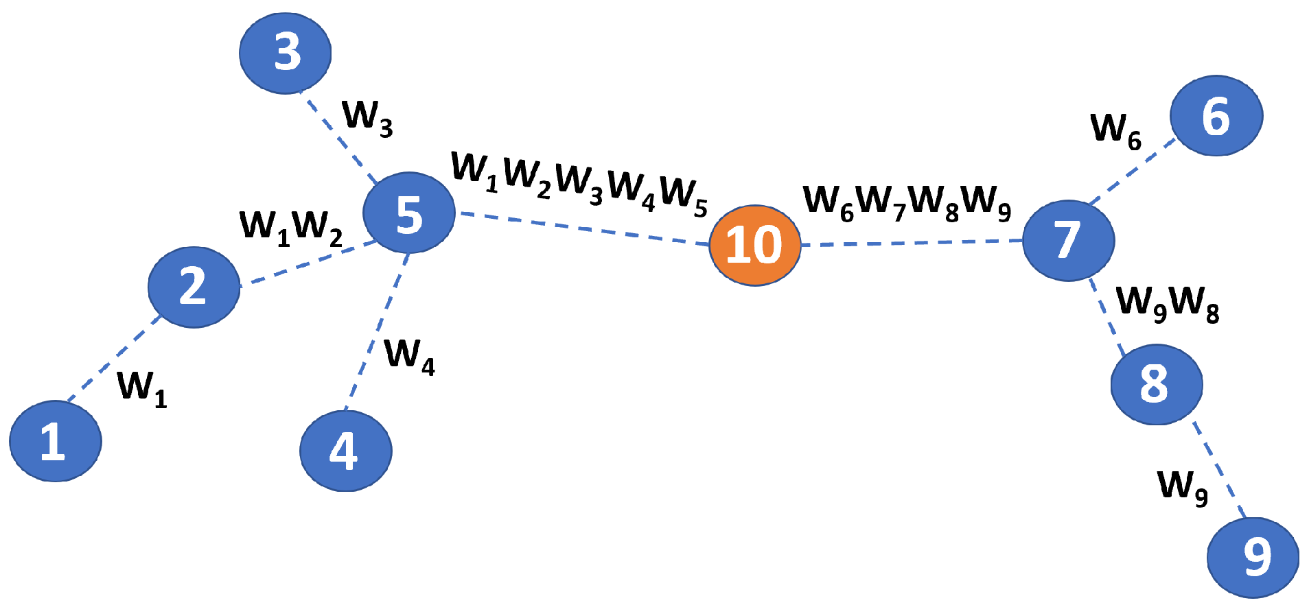
This averaged model is then re-disseminated to all of the learners and retrained locally. After a few iterations, a final common model is achieved. The efficacy of FL has been discussed thoroughly, although the drawbacks associated with the numerous iterations [7] have emerged. Indeed, FL can be very costly in terms of the number of data being forwarded throughout the network. As an example, in Figure 1 we report a network topology where the use of FL in its traditional implementation is very inefficient. The network in Figure 1 consists of 10 nodes. Nodes 1 to 9 are the learners, and node 10 is the aggregation point. Note that models elaborated by learners will traverse multiple hops to reach node 10. This is very costly in terms of the use of network resources.
Another non negligible drawback related to the use of standard FL is associated with the excessive exhaustion of energy resources at those nodes located close to the aggregation point. This is a well-known networking problem, which is referred to as funneling effect [8]. As an example, nodes 7 and 5, which are just one hop away from the aggregation point, are subject to excessive traffic associated with relaying the model parameters of the peripheral nodes. The use of partial model aggregations at the intermediate nodes can be effective, although it requires extra overhead and awareness of a route towards the final aggregation point. To cope with these limitations, gossiping has been recently considered. It consists of a distributed consensus mechanism that exploits local computing resources to limit the data transmitted across the network. The main advantages of gossiping are also related to the consequent efficiency in decreasing energy consumption and a waste of communication resources, with a positive effect on latency and network lifetime [9,10,11]. Advantages related to the use of gossiping in WSNs have been analyzed in [12,13], with a particular focus on distributed inference and detection. Additionally, in [14,15,16,17,18], the use of gossiping combined with FL for the purpose of solving a consensus problem in the framework of ML model weights has been proposed. The use of gossiping under has been analyzed theoretically in [19], where the control of the communication time is achieved by tuning the nodes transmission rates and modifying the network topology, consequently. An interesting recent work that discusses the use of gossiping and federated learning with consideration of network constraints is presented in [20].
As compared to the previous literature in the field, in this paper we tradeoff multiple aspects in network design. On the one hand, we consider performing ML operations in a WSN, and toward this aim we present a distributed learning approach that combines federated learning and gossiping. Additionally, from a networking point of view, we assume that WSN nodes are battery powered and, in general, have heterogeneous computing capabilities. Accordingly, we design a clustering algorithm where a few nodes, i.e., one per cluster, perform model training, while all of the others execute inference only. Then, to guarantee fairness and avoid the overload of a few nodes only along with the consequent exhaustion of their batteries, we propose a mechanism for cluster-head role rotation. Finally, in order to improve the model parameter dissemination process, the proposed mechanism is aware of the centrality of network nodes. The objective is to foster model parameter dissemination performed by nodes that have privileged positions in the topology of the network.
The main contributions and the novelty of our proposed approach when compared to the previous solutions are as follows:
- A clustering scheme for collaborative learning in WSNs that exploit the gossiping mechanism to exchange model parameters between clusters.
- The consideration of the machine learning capabilities, the residual energy, the centrality information, and the transmission power of the nodes to improve the fairness and speed up the convergence.
- An intelligent scheme to transmit data chunks from cluster heads to cluster members only when it is necessary to reduce the communication load, at the same time enhancing the collaborative learning.
Our proposed approach can be exploited in WSNs consisting of low-power devices that can only run inference, such as TensorFlow Lite [21].
The rest of this paper is organized as follows. In Section 2, we discuss the recent works on exploiting clustering in FL. In Section 3, we present the CINE algorithm by detailing the network protocol and the approaches used to include centrality. In Section 4, we assess the proposed protocol. Finally, in Section 5 some conclusions on the work are drawn.
2. Related Work
In this section, we will discuss the recent works that are most relevant to our proposed approach. More specifically, We will discuss the distributed learning approaches, especially model-aggregation-based schemes in which clustering is exploited.
In [22], the authors propose a FL scheme by combining FL and hierarchical clustering with separate clusters of devices according to the similarity of their local mode updates to the global joint model. After the separation, the clusters in the network are trained independently. The authors compared the performance of their proposed approach with the approach in which clustering is not exploited and observed that the model training in the proposed approach converged in fewer communication rounds.
Similarly, in [23], the authors proposed a similarity aware FL scheme that can contribute high model accuracy for human-activity recognition applications. The scheme has a clustering FL framework that captures the relationship among the data of different nodes. Upon learning the cluster relationship, the nodes that converge more slowly can be dropped to speed up the convergence. The proposed scheme was evaluated on an NVIDIA edge testbed using human-activity recognition data collected from a total of 145 users.
In [24], the authors develop a clustering-based FL framework that groups into multiple clusters. Each communication round of the framework consists of multiple cycles of meta-update to speed up the overall convergence. Experiments were conducted exploiting deep learning algorithms to show that the proposed framework achieves convergence significantly faster than the standard FL approach.
Another clustering-based FL approach is proposed in [25] in which the geometric properties of the FL loss surface are considered to group the devices into clusters. Thus, each cluster has devices with jointly trainable data distributions. The proposed scheme is designed to preserve privacy and can handle numerous client devices that vary over time.
Though many clustering-based schemes have been proposed in the literature to enhance FL, their main objective has been grouping devices based on either similarity in terms of data or in terms of model parameters. In our work, we developed a decentralized scheme that is based on grouping nodes such that a central node, also known as the cluster head, in the cluster has higher machine learning and communication capabilities than other nodes. The role of the central node is rotated to achieve fairness in the network. The chosen cluster head broadcasts its model parameters to the cluster members. The cluster members that received the model parameters aggregate the received model parameters with their own model parameters, as is done in FL. We discuss the recent works in which gossiping is combined with FL to reduce the consumption of energy and communication resources.
In [16,17], the authors introduce an integrated networking/learning approach for WSNs by combining FL with gossiping. The proposed approach enables the nodes to perform model aggregation locally instead of transmitting the model parameters to the central aggregation point for aggregation. Similarly, the authors in [18] develop a centrality aware gossiping protocol distributed learning in WSNs. The nodes exploit the centrality information to enhance the collaborative learning of the model. More specifically, the centrality information is exploited in the algorithm that is designed for identifying the nodes that are supposed to broadcast their model parameters in each communication round. It was observed that the proposed approach performs significantly better with the inclusion of the centrality information. Similarly, the authors in [20] propose a server-less consensus based learning approach for massive IoT networks. The proposed approach is assessed using data collected in an industrial IoT environment. In our work, we exploit the gossiping mechanism but in a clustering manner by considering the ML and transmission capabilities of the node along with the energy consumption.
3. CINE Solution
In the following sections, we will first present an overview of the CINE protocol, and then we will detail the different algorithms employed for addressing a multicriteria-based distributed learning optimization problem.
3.1. Overview of CINE
Considering the intrinsic limitations of WSN devices and the limited computational and energy capabilities, we have designed and implemented a methodology that allows one to guarantee network efficiency trading off lifetime and reliability.
More specifically, we assume to have a WSN where nodes have severe resource limitations. Although the support of solutions for the execution of machine learning in WSNs has been advocated in the recent past [1], to cope with limited node capabilities, we use clusters inside the network and the selection of few cluster representative nodes to simplify the problem of device model training.
Accordingly, we assume that only a few nodes, denoted as cluster heads (CHs), perform training, while other cluster nodes, denoted as cluster members (CMs), execute inference by only applying the model disseminated by their CH. In order to balance the consumption of energy and processing resources, we let the CH role, which is the most demanding in terms of energy consumption, rotate among nodes belonging to the same cluster. Accordingly, we introduce a CH selection mechanism. The mechanism considers that regions have been defined in the network area and that a cluster consists of all nodes located in a given region. Regions are defined by exploiting the statistical knowledge of node distribution in the area so that the number of nodes in all of the clusters is approximately the same. Let be the average number of nodes in a cluster. Note that the detailed policies for the identification of clusters and the consequent selection of cluster members is out of the scope of the current paper. For an extensive discussion of the design of clustering algorithms for ad hoc and sensor networks that are guaranteed to have an assigned number of cluster members, please refer to [26].
We assume that each node has the information required to identify its cluster at its startup phase. This can be easily achieved by using position information along with the awareness of the above-mentioned cluster regions. The first node joining the cluster will be the initial cluster head. We define a time window duration as , which represents the interval during which the cluster head does not change and is a constant known to all of the network nodes.
At the end of the window, the current cluster head broadcasts a COMPETITION_INITIATION message to all cluster members by applying any appropriate geocast mechanism [27], to identify the CH for the next time window. This starts a competition phase that lasts for a time interval equal to . The appropriateness of the j-th node for the CH role is related to a number of parameters, such as its residual energy (), its centrality ( discussed later in Section 3.2), and its computing capabilities (). Each node j, after evaluating a penalty value, , will answer back by broadcasting the value of its penalty inside a COMPETITION_TERMINATION message, which also carries the sender ID, i.e., j. The broadcast will be executed at a time where is a a random variable generated according to a probability distribution whose average is proportional to . In this way, nodes with smaller values (i.e., a lower penalty) will answer before the others. Other cluster members, upon hearing the COMPETITION_TERMINATION message, will not answer back and identify the new CH as the sender of the COMPETITION_TERMINATION message.
For the following interval, the CH will remain unchanged. During this interval, training will be executed only by the CH, while cluster members will only perform inference. In case the residual energy at a CH decreases below a threshold, , before , a new competition procedure will be triggered to identify a new CH. This will be done through a COMPETITION_REQUEST message sent by the CH node.
After , a new competition will be triggered inside the cluster to identify which node will be the next CH. To this aim, the current CH transmits a COMPETITION_TRIGGER message. Upon receiving it, each cluster member j updates the estimate of the relevant values, i.e., its residual energy, ; its computing capabilities, ; its centrality, ; and the loss of the current ML model, , needed to estimate the penalty . Similarly to the case of the initial competition, a node j will schedule the transmission of a COMPETITION_TERMINATION message containing the value of , as well as its identifier inside at time where is a random variable with average proportional to . Based on this choice, nodes with low penalty will answer before, and the best node will serve as the new CH for at most a time .
Note that, as detailed in the following section, CHs in different clusters form a so-called CH-network. This network connects all CHs of different clusters according to a mesh topology. When a node q emerges as the new CH of the cluster , i.e, , it sets a higher TX power and broadcasts a CH_NETWORK_NOTIFICATION message carrying its identifier, as well as the ID of the previous node that acted as CH for the same cluster . In this way, all CH nodes that receive this message will update their current list of CH-network members by considering node q as the new . Correspondingly, they will update their cluster member list by now considering the previous CH as a simple cluster member.
The procedure for cluster management is sketched in Algorithm 1.
| Algorithm 1 Protocol-Cluster Management |
|
3.2. Centrality
As discussed in the previous section, we use centrality to characterize the topological relevance of a node inside a cluster and the relationship it has with neighbouring nodes. In the recent past, the use of centrality in WSNs has been considered as a powerful tool to perform cluster-head selection [28] in order to increase network lifetime and, in general, reduce energy consumption [29]. Additionally, centrality has been exploited to achieve efficient routing, prolong network lifetime [30,31], and facilitate data fusion. Multiple centrality metrics have been considered in the literature for WSNs, as reported in [32]. Indeed, the most of those used are degree centrality, betweenness centrality, eigen centrality, and closeness centrality.
The simplest centrality metric that is often used for clustering is degree centrality. It, in particular, evaluates the number of links owned by a given network node. betweenness centrality identifies the number of times a node lies on the shortest path between all of the possible pairs of nodes. eigen centrality calculates the topological relevance of a node by estimating the number of links it has with the other nodes in the network. Additionally, this metric considers the number of connections of the nodes to which a given node is connected on its own. This type of approach is, for example, used in Google Pagerank and Katz centrality [33]. Another variant of centrality is the so called closeness centrality, which evaluates the geodesic distance between a node and all of the other nodes in the network. Unlike betweenness centrality, closeness centrality estimates how short the shortest paths are between the node and all other nodes.
In this paper, we design a clustering methodology that is driven by centrality awareness, energy efficiency, and the consideration of the computing and processing capabilities of nodes for performing distributed learning in WSNs. The approach, as discussed in the following, will prove to efficiently trade off contrasting features, leading to fast convergence and an increase in network lifetime as compared to static and capability-unaware distributed learning solutions.
3.3. Distributed Learning and Gossiping
In this section, we detail the protocol executed by WSN nodes to perform distributed learning and gossiping.
We assume that all of the network nodes have the capability to set the transmission power to:
- The low power TX mode, used when a node (either a CH or a simple CM) communicates with other nodes of the same cluster;
- The high power TX mode, used when a CH node communicates with other CH nodes in the CH-network.
Cluster heads perform model training using their own data. The fitness of the ML model is evaluated through an appropriate loss function hl (The choice of a specific loss function is out of the scope of this work. In the literature, several loss functions have been introduced for different application scenarios. A comprehensive overview is available in [34]).The loss for a specific node j is indicated as .
Upon estimating its model loss on the completion of a training execution, each cluster head communicates this value across the CH-network. Based on this dissemination, all of the CHs know the loss functions of the others. Thus, before starting a new competition, the CH declaring the lowest loss function value will transmit its model parameters to its one-hop neighbors in the CH-network using the high power TX mode.
Upon receiving the model issued by a generic CH j, the k-th cluster head will use the received model parameters, , to update its own model, , as follows:
where is a weight parameter that allows one to characterize the trust the CH node has in the other CHs. Then, the CHs retrain the model obtained applying Equation (1) using the data that are locally available.
In order to preserve the energy consumption inside each cluster, cluster members are not required to execute the training, although they can in principle; they only perform inference. More specifically, the CH of cluster takes care of training the model that is transmitted and used for inference by the other cluster members to be broadcast to all of the cluster members of cluster , together with the value of its corresponding loss .
Upon receiving the weight model from the CH, the CMs will estimate their loss based on the updated model using their own data. A cluster member of cluster that obtains a loss higher then the value contained in the message transmitted by the CH, , plus a given threshold, , will send a chunk of its data to the CH for retraining. The CH will retrain the model using the received data chunk. In this way, the updated model will be efficient and will also be representative of the data of other CMs.
The execution of the above set of operations is denoted as protocol iteration. After each iteration, the involved CH will broadcast its updated loss value throughout the CH-network so that all of the other CHs can compare it to their own loss values.
3.4. Protocol Details
In this section, we briefly illustrate how the protocol works.
Algorithm 2 represents the pseudocode for the protocol run by the generic CH.
| Algorithm 2 CINE Protocol-Cluster Head Functioning |
|
At the startup, the model is trained by the CH using the local data and starting from random initial conditions, RND. Let be the resulting loss. Such value will be used, along with the residual energy and the information regarding available computing capabilities, to calculate the penalty parameter as follows:
where is the loss of the CH, is its degree centrality, is its residual energy, and is its computing capability.
To conclude the initialization phase, the cluster head broadcasts the model parameters of the obtained model in the cluster. Moreover, it broadcasts the value of its penalty in the CH-network. This last operation is needed to allow for identification among the CHs of the node that exhibits the lowest penalty , which will then send its model parameters to the neighboring CHs in the CH-network.
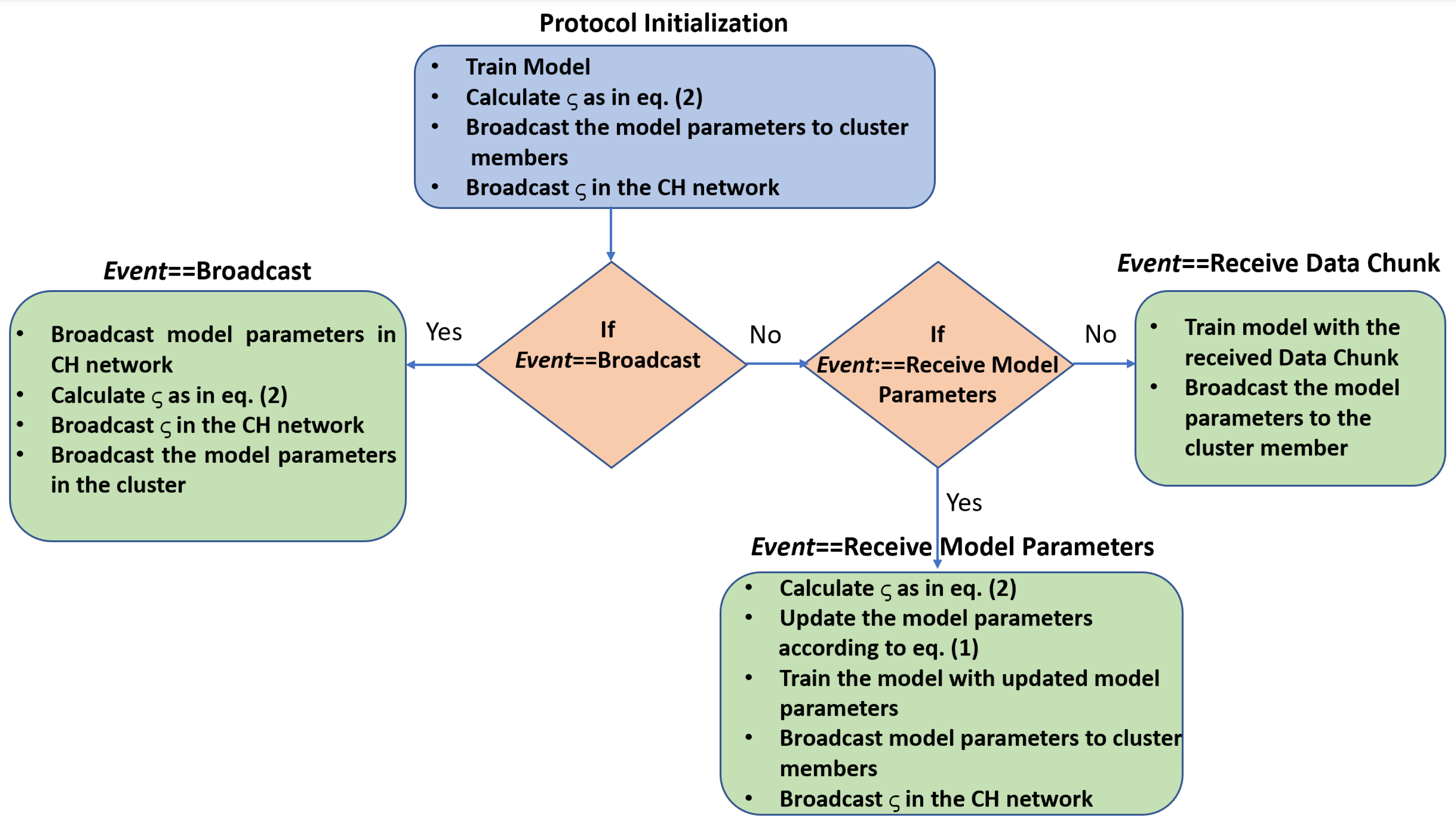
After the initialization phase, regular operations are executed that are the consequence of three types of events:
- Broadcast: The cluster head exhibiting the lowest penalty broadcasts its model parameters to both its cluster members and its neighboring CHs.
- Receive Model Parameters: upon receiving the model parameters by another cluster head (i.e., the one exhibiting the lowest penalty), the CH retrains the model.
- Receive Data Chunk: The CH that receives a chunk of data from a CM includes it in its local data set and retrains the model. In this way, the new model is representative of a more comprehensive data set.
For what concerns the operations performed by cluster members, we observe that they are straightforward consequences of what we have described so far. Upon receiving the model parameters sent by its cluster head, a generic cluster member estimates the loss obtained by using such a model. If the difference between the loss just calculated and the loss declared by the CH is larger than a given threshold , it sends a chunk of its data to the CH for retraining.
4. Performance Evaluation
In this section, we assess the performance of CINE. Accordingly in the following section, i.e., Section 4.1, we describe the WSN scenario and the data set considered in our experiments. Then, in Section 4.2, we present and discuss the numerical results.
4.1. Simulation Scenario
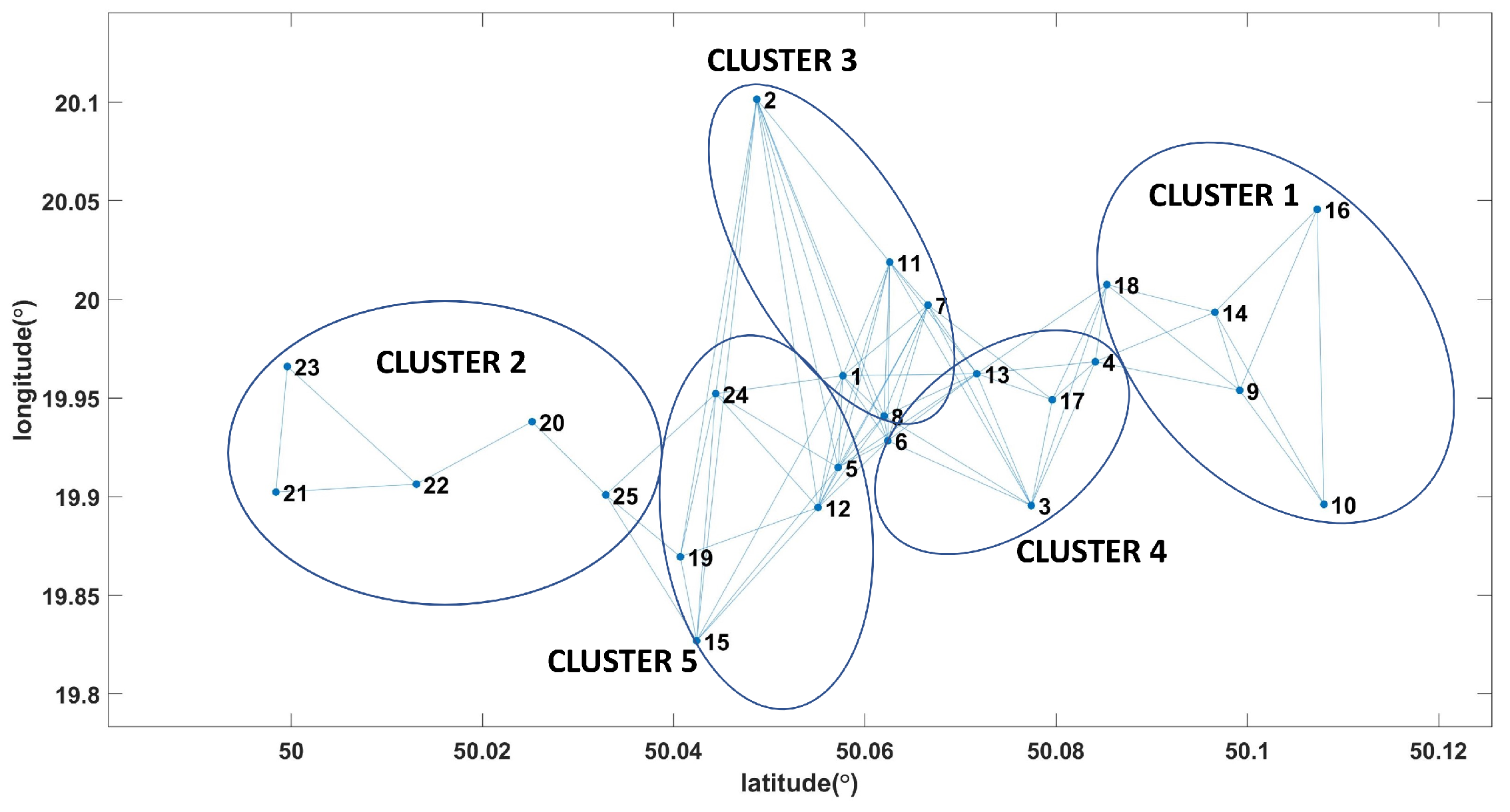
For the simulation experiments, we considered a well-known data set containing air-quality sensor data measured by a sensor network consisting of 56 nodes deployed in the city of Krakov https://www.kaggle.com/datascienceairly/air-quality-data-from-extensive-network-of-sensors (accessed on 12 March 2023). We considered the 25 nodes that provided a complete set of sensor data for a period of one month.
In Figure 3, we report the position of the nodes and the resulting topology of the WSN.
The sensors collect one sample of measures every hour; therefore, the data set for one month (i.e., 30 days) for each of the 25 sensors consists of entries, with . Each entry includes seven values, representing the day; time; temperature; humidity; and PM1, PM2.5, and PM10 values. Note that the day and time values are not included for training the model, and thus the seven parameters reduce to five only. For the training in cluster heads, 25 days of data are considered for training. For the inference in both cluster heads and inference, the last 5 days of data are considered for inference. Thus, for training, the data set corresponding contains 25 (days) × 24 (h) = 600 entries of temperature; humidity; and PM1, PM2.5, and PM10 values. For the inference, the data set corresponding to each sensor contains 5 (days) × 24 (h) = 120 entries of temperature; humidity; and PM1, PM2.5, and PM10 values. The data chunk that has to be transmitted to the cluster head for retraining also comprises 5 days of data. Accordingly, the u-th entry in the data set of the k-th sensor, denoted as , is:
CINE can been applied whatever the ML approach utilized. For our experiments, we considered the well-known convolutional autoencoders, which are usually applied for dimension reduction, denoising, and anomaly detection [35,36,37,38,39].
They consist of convolutional neural networks (CNNs), both at the encoder and at the decoder. Readers interested in gaining a deeper understanding of convolutional autoconders can refer to [40,41,42,43].
We built a model with two convolutional layers in the encoder part and two deconvolutional layers in the decoder part. All the four layers were one-dimensional convolutional layers. The 8 × 8 kernels and ReLU activations were used. The outer layers of the model consist of 32 filters, while the inner layers consist of 16 filters. The model takes the input of shape (batch_size, sequence_length, num_features) and returns the output of the same shape. In our experiments, we varied the sequence_length from 25 to 100, and num_features was set to 1. The sequences consisted of the timeseries sequences of the sensor values from the dataset.
4.2. Numerical Results
In this section, we report the numerical results obtained in the scenario described in the previous section by applying the CINE protocol. We conducted large simulation campaigns to estimate the average loss with respect to the number of iterations for different types of centrality, , and threshold, , values. We also evaluated the average residual energy at each cluster. Note that the residual energy was evaluated in terms of percentage for generalizing the exploitation of any kind of short-range (low TX power)/long-range radios (high TX power) in a WSN scenario. We assumed that the node exploits the bluetooth low energy for the short-range radio (the low-power TX mode case) and LoRa for the long-range radio (the high-power TX mode case). Since bluetooth low energy has a power consumption of 50mW and LoRa has a power consumption of 150 mW [44,45], we considered the energy consumption in the long-range radio to be 10 times that of the power consumption in the short-range radio as both bluetooth low energy and LoRa can communicate at the same data rate in specific settings.
Finally, we calculated the average number of data chunk transmissions with respect to different threshold values. Note that the loss metric considered in this paper is the medium square error (MSE), which is calculated as
where y is the input data fed into the autoencoder, is the reconstructed output data, and is the length of the input data.
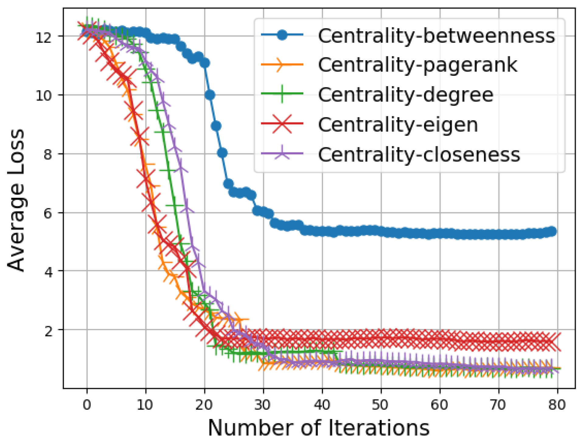
In Figure 4, we report the average loss with respect to the number of iterations for different centrality metrics. We observe that the eigen, pagerank, and degree centrality metrics give similar results, while the average loss in the case of betweenness centrality is significantly higher. Accordingly, in this section we will present the results achieved by applying the degree centrality. In fact, eigen and pagerank centrality give similar results, whereas betweenness centrality gives much worse results and thus must be excluded.
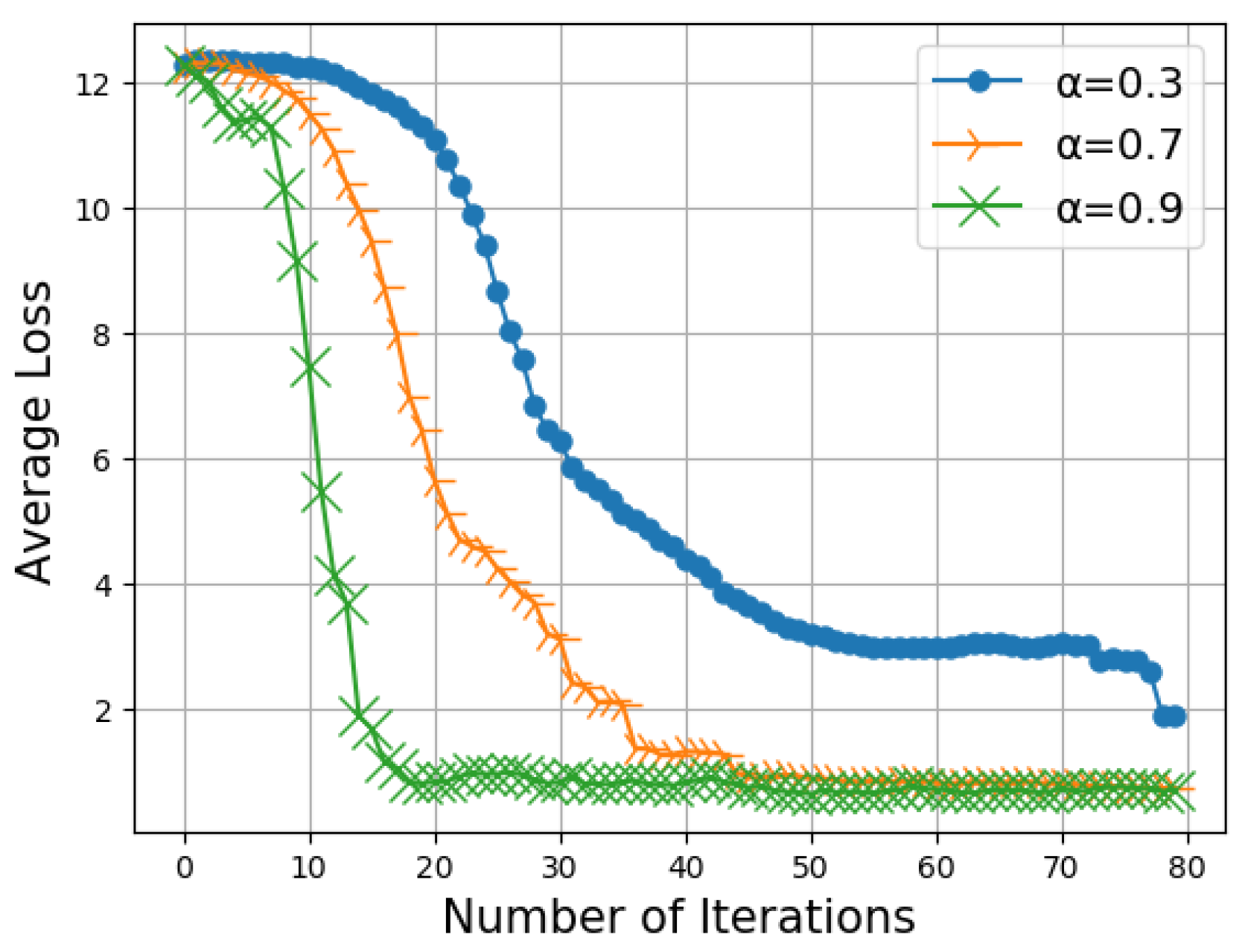
In Figure 5, we report the average loss with respect to the number of iterations for different values of . Note that is the parameter that weights the importance given by each CH to the models received by another CH, as given in Equation (1). From Figure 5, we observe that the convergence is faster when the is higher. corresponds to the tuning parameter in the weight update Equation (1). If the value of is higher, it means more priority is given to the model parameters that were just received than the nodes current model parameters. If the value is lower, it means that less priority is given to the model parameters that were just received than the nodes current model parameters. From Figure 5, it is observed that the convergence is faster when higher weightage is given to the model parameters that were received by the nodes.
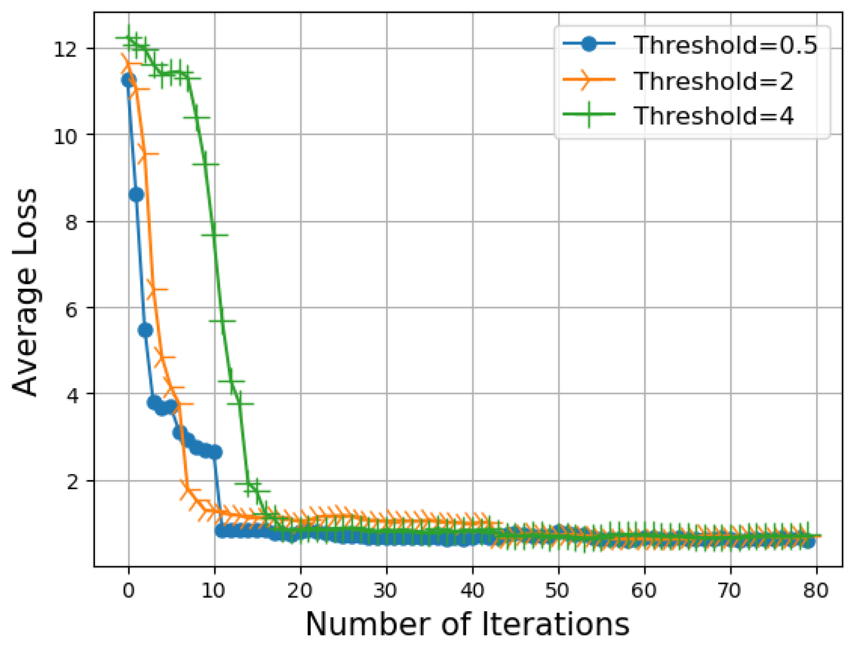
In Figure 6, we report the average loss with respect to the number of iterations for different values of the threshold . In the first 20 iterations, the average loss decreases quickly when the threshold is low. The reason for this occurrence is that the data chunk transmissions are more frequent when the threshold is low; therefore, the models are trained considering more data. More specifically, a lower threshold will result in the high frequency of transmission of data chunks from the cluster members to the cluster heads. This will enable the cluster head to train with more data. Hence, the performance of the model is enhanced, resulting in lower average loss.
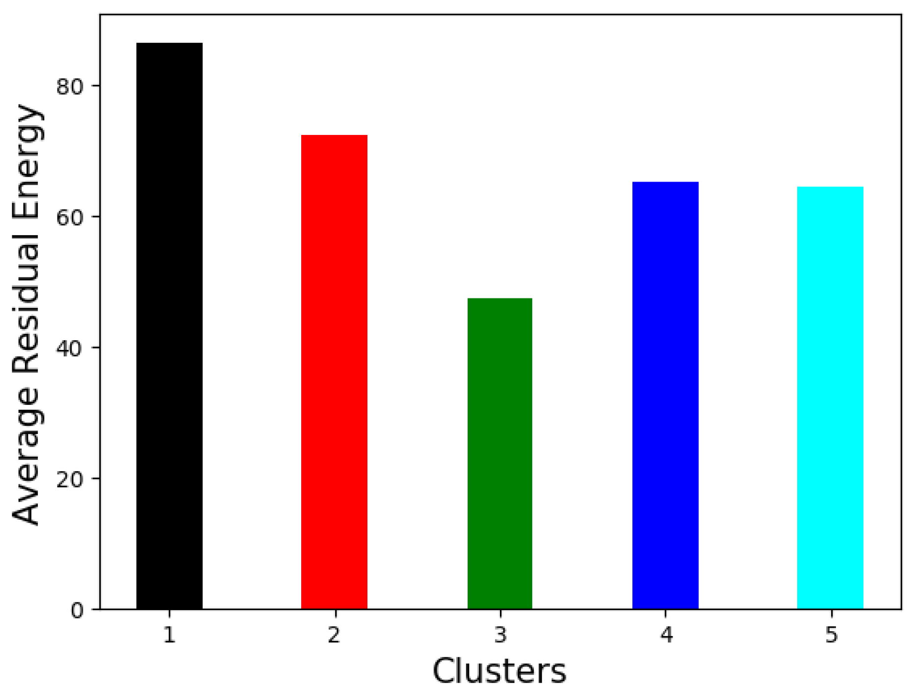
In Table 1, we report the average residual energy at each cluster after 80 iterations. Clusters 1 and 2 have higher residual energy after 80 iterations than Clusters 3, 4, and 5. In the same table, we report the standard deviation of the residual energy in each cluster and, for the sake of comparison, we report the standard deviation of the residual energy that would be obtained without considering the multi-criteria definition of the penalty . We observe that by applying the proposed approach, significantly lower standard deviation values are obtained, which means that there is an improvement in fairness.
Note that Clusters 1 and 2 comprise nodes with lower centrality values. On the contrary, Cluster 3 in the center of the network comprising nodes with higher centrality metrics also has the lowest residual energy when compared to the other clusters.
In Figure 7, we report the average residual energy versus the number of iterations for different values of threshold . Obviously, the residual energy increases when the threshold value increases. This is because by increasing the threshold, the number of chunk transmissions decreases. This is confirmed by the values in Table 2.
Therefore, from the obtained numerical results, we derive that the residual energy and centrality metrics play an important role in enhancing the distributed learning in a network.
In Figure 8, we show the average residual energy in each cluster. We observe that cluster ‘3’ has consumed higher energy than the other clusters. This can also be seen in Figure 9, where we show the residual energy in each node. The residual energy is lower in cluster ‘3’ as the nodes in cluster are in the center of the network with higher centrality values. Thus, they have the opportunity to gossip about the model parameters a few times more than the nodes in other clusters. Similarly, the nodes in cluster ‘1’ exhibit higher energy consumption as they are not well connected like the other nodes, and they have lower centrality values. This shows how the centrality of the nodes can affect the energy consumption of the nodes.
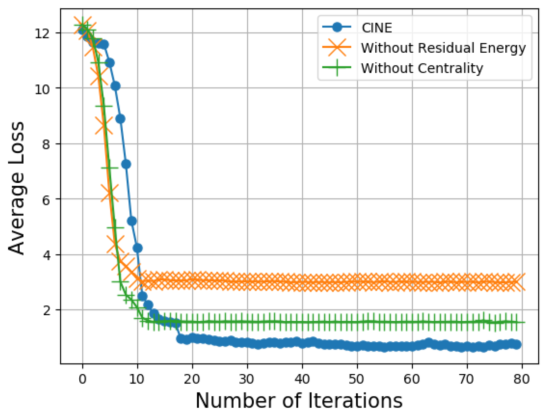
In Figure 10, we compare CINE with other cases in which we exploit neither the centrality information nor the residual energy information. On comparing the three cases, we observe that our CINE protocol that exploits both the centrality and the residual energy information outperforms the cases in which either the the centrality information or the residual energy information is not utilized. Though the average loss obtained by CINE is comparatively higher in the initial iterations, the average loss reduces significantly after 10 iterations and converges quickly when compared to the other two cases without the centrality information or the residual energy information.
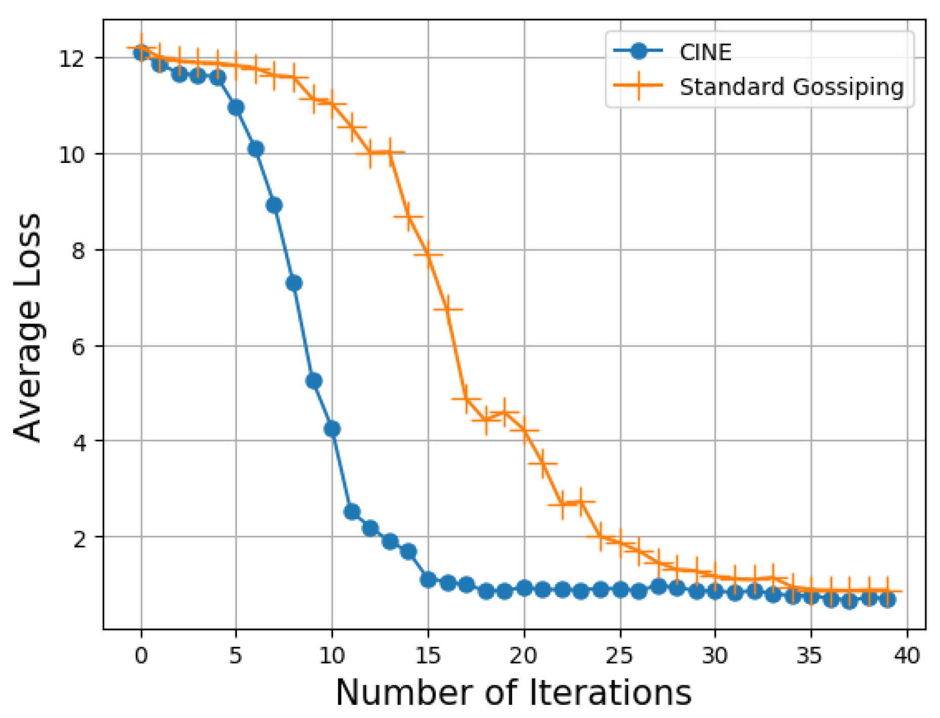
Furthermore, we compare CINE with an ordinary gossiping approach in Figure 11. In case of ordinary gossiping, each node is selected as a cluster head to periodically broadcast the model parameters (we call this approach standard gossiping). We show the average loos with respect to the number of iterations for both CINE and the standard gossiping. It is evident that the performance in CINE is significantly better than the standard gossiping. As observed, the average loss obtained CINE falls below 2 after 12 iterations, whereas the average loss in the case of standard gossiping falls below 2 only after 24 iterations. This demonstrates the satisfactory learning features of the CINE protocol.
5. Conclusions
In this paper, we have proposed the CINE protocol for distributed learning in WSNs. CINE exploits clustering and uses a multi-parametric approach to distribute the computation and communication load between all nodes in the cluster. CINE is designed by considering the energy and machine learning capabilities of the nodes. More specifically, wireless sensor nodes are partitioned in clusters, and a cluster head is selected in each cluster that can execute both training and inference, whereas the cluster members are responsible for executing only the inference. Since the cluster heads consume more resources than the cluster members, our proposed protocol rotates the cluster head role among all of the nodes in the cluster. Simulation experiments were carried out using the CNN auto-encoder model on a well-known data set containing air-quality sensor data measured by a sensor network. The numerical results show that by considering the node centrality information and the residual energy information, CINE has the potential to achieve convergence at a faster rate and improve the fairness in the distributed learning. The CINE protocol can be exploited in WSN scenarios where nodes have different communication, machine learning, and energy capabilities. CINE represents very efficient scenarios where ML models have to deploy low-power devices.
Author Contributions
Conceptualization L.G., J.S.M. and G.M.; methodology, L.G., J.S.M. and G.M.; software, J.S.M.; validation, L.G., J.S.M. and G.M.; formal analysis, L.G. and G.M.; investigation, L.G., J.S.M. and G.M.; resources, L.G., J.S.M. and G.M.; data curation, J.S.M.; writing—original draft preparation, L.G., J.S.M. and G.M.; writing—review and editing, L.G., J.S.M. and G.M.; visualization, J.S.M.; supervision, L.G.; project administration, none; and funding acquisition, L.G. and G.M. All authors have read and agreed to the published version of the manuscript.
Funding
This paper was partially supported by the Sicilian Region under the project SAFE-DEMON and MUR under the project Liquid Edge.
Acknowledgments
This paper was partially supported by the Sicilian Region under the project SAFE-DEMON, the MUR under the project Liquid Edge and the European Union (NextGeneration EU), through the MUR-PNRR project SAMOTHRACE (ECS00000022).
Conflicts of Interest
The authors declare no conflict of interest.
References
- Alsheikh, M.A.; Lin, S.; Niyato, D.; Tan, H.P. Machine Learning in Wireless Sensor Networks: Algorithms, Strategies, and Applications. IEEE Commun. Surv. Tutor. 2014, 16, 1996–2018. [Google Scholar] [CrossRef]
- Peteiro-Barral, D.; Guijarro-Berdiñas, B. A survey of methods for distributed machine learning. Prog. Artif. Intell. 2013, 2, 1–11. [Google Scholar] [CrossRef]
- Predd, J.B.; Kulkarni, S.B.; Poor, H.V. Distributed learning in wireless sensor networks. IEEE Signal Process. Mag. 2006, 23, 56–69. [Google Scholar] [CrossRef]
- Danaee, A.; de Lamare, R.C.; Nascimento, V.H. Energy-efficient distributed learning with coarsely quantized signals. IEEE Signal Process. Lett. 2021, 28, 329–333. [Google Scholar] [CrossRef]
- Carpentiero, M.; Matta, V.; Sayed, A.H. Distributed Adaptive Learning under Communication Constraints. arXiv 2021, arXiv:2112.02129. [Google Scholar]
- Niknam, S.; Dhillon, H.S.; Reed, J.H. Federated Learning for Wireless Communications: Motivation, Opportunities, and Challenges. IEEE Commun. Mag. 2020, 58, 46–51. [Google Scholar] [CrossRef]
- Luo, B.; Li, X.; Wang, S.; Huang, J.; Tassiulas, L. Cost-Effective Federated Learning Design. arXiv 2020, arXiv:cs.LG/2012.08336. [Google Scholar]
- Sen, P. Funnelling Effect in Networks. In Proceedings of the International Conference on Complex Sciences, Shanghai, China, 23–25 February 2009. [Google Scholar]
- Dimakis, A.G.; Kar, S.; Moura, J.M.F.; Rabbat, M.G.; Scaglione, A. Gossip Algorithms for Distributed Signal Processing. Proc. IEEE 2010, 98, 1847–1864. [Google Scholar] [CrossRef]
- Shah, D. Gossip Algorithms. Found. Trends Netw. 2009, 3, 1–125. [Google Scholar] [CrossRef]
- Boyd, S.; Ghosh, A.; Prabhakar, B.; Shah, D. Randomized gossip algorithms. IEEE Trans. Inf. Theory 2006, 52, 2508–2530. [Google Scholar] [CrossRef]
- Kar, S.; Moura, J. Consensus-based detection in sensor networks: Topology optimization under practical constraints. In Proceedings of the 1st International Workshop on Information Theory in Sensor Networks, Santa Fe, NM, USA, 18–20 June 2007. [Google Scholar]
- Saligrama, V.; Alanyali, M.; Savas, O. Distributed Detection in Sensor Networks with Packet Losses and Finite Capacity Links. IEEE Trans. Signal Process. 2006, 54, 4118–4132. [Google Scholar] [CrossRef]
- Blot, M.; Picard, D.; Cord, M.; Thome, N. Gossip Training for Deep Learning. arXiv 2016, arXiv:cs.CV/1611.09726. Available online: http://xxx.lanl.gov/abs/1611.09726 (accessed on 13 March 2023).
- Daily, J.; Vishnu, A.; Siegel, C.; Warfel, T.; Amatya, V. GossipGraD: Scalable Deep Learning Using Gossip Communication Based Asynchronous Gradient Descent. arXiv 2018, arXiv:cs.DC/1803.05880. [Google Scholar]
- Mertens, J.S.; Galluccio, L.; Morabito, G. Federated learning through model gossiping in wireless sensor networks. In Proceedings of the 2021 IEEE International Black Sea Conference on Communications and Networking (BlackSeaCom), Bucharest, Romania, 24–28 May 2021. [Google Scholar]
- Mertens, J.S.; Galluccio, L.; Morabito, G. MGM-4-FL: Combining federated learning and model gossiping in WSNs. Comput. Netw. 2022, 214, 109144. [Google Scholar] [CrossRef]
- Mertens, J.S.; Galluccio, L.; Morabito, G. Centrality-aware gossiping for distributed learning in wireless sensor networks. In Proceedings of the 2022 IFIP Networking Conference (IFIP Networking), Catania, Italy, 13–16 June 2022. [Google Scholar]
- Lalitha, A.; Kilinc, O.C.; Javidi, T.; Koushanfar, F. Peer-to-Peer Federated Learning on Graphs. arXiv 2019, arXiv:cs.LG/1901.11173. [Google Scholar]
- Savazzi, S.; Nicoli, M.; Rampa, V. Federated Learning With Cooperating Devices: A Consensus Approach for Massive IoT Networks. IEEE Internet Things J. 2020, 7, 4641–4654. [Google Scholar] [CrossRef]
- Dokic, K.; Martinovic, M.; Mandusic, D. Inference Speed and Quantisation of Neural Networks with TensorFlow Lite for Microcontrollers Framework. In Proceedings of the 2020 5th South-East Europe Design Automation, Computer Engineering, Computer Networks and Social Media Conference (SEEDA-CECNSM), Corfu, Greece, 25–27 September 2020; pp. 1–6. Available online: https://doi.org/10.1109/SEEDA-CECNSM49515.2020.9221846 (accessed on 12 March 2023).
- Briggs, C.; Fan, Z.; Andras, P. Federated Learning with Hierarchical Clustering of Local Updates to Improve Training on Non-IID Data. In Proceedings of the 2020 International Joint Conference on Neural Networks (IJCNN), Glasgow, UK, 19–24 July 2020; pp. 1–9. [Google Scholar] [CrossRef]
- Ouyang, X.; Xie, Z.; Zhou, J.; Huang, J.; Xing, G. ClusterFL: A Similarity-Aware Federated Learning System for Human Activity Recognition. In Proceedings of the MobiSys ’21: 19th Annual International Conference on Mobile Systems, Applications, and Services, Virtual, 24 June–2 July 2021; Association for Computing Machinery: New York, NY, USA, 2021; pp. 54–66. [Google Scholar] [CrossRef]
- Chen, C.; Chen, Z.; Zhou, Y.; Kailkhura, B. FedCluster: Boosting the Convergence of Federated Learning via Cluster-Cycling. In Proceedings of the 2020 IEEE International Conference on Big Data, Atlanta, GA, USA, 10–13 December 2020; pp. 5017–5026. [Google Scholar] [CrossRef]
- Sattler, F.; Müller, K.R.; Samek, W. Clustered Federated Learning: Model-Agnostic Distributed Multitask Optimization Under Privacy Constraints. IEEE Trans. Neural Netw. Learn. Syst. 2021, 32, 3710–3722. [Google Scholar] [CrossRef]
- Al-Sulaifani, A.I.; Al-Sulaifani, B.K.; Biswas, S. Recent trends in clustering algorithms for wireless sensor networks: A comprehensive review. Comput. Commun. 2022, 191, 395–424. [Google Scholar] [CrossRef]
- Jiang, X.; Camp, T. A Review of Geocasting Protocols for a Mobile ad Hoc Network. Available online: https://citeseerx.ist.psu.edu/document?repid=rep1&type=pdf&doi=7a515b48994384dd95439cbc4d4584af993b2a49 (accessed on 12 March 2023).
- Gupta, I.; Riordan, D.; Sampalli, S. Cluster-head election using fuzzy logic for wireless sensor networks. In Proceedings of the 3rd Annual Communication Networks and Services Research Conference (CNSR’05), Halifax, NS, Canada, 16–18 May 2005. [Google Scholar] [CrossRef]
- Aditya, V.; Dhuli, S.; Sashrika, P.L.; Shivani, K.K.; Jayanth, T. Closeness centrality Based cluster-head selection Algorithm for Large Scale WSNs. In Proceedings of the 2020 12th International Conference on Computational Intelligence and Communication Networks (CICN), Bhimtal, India, 25–26 September 2020; pp. 107–111. [Google Scholar] [CrossRef]
- Oliveira, E.M.R.; Ramos, H.S.; Loureiro, A.A.F. Centrality-based routing for Wireless Sensor Networks. In Proceedings of the 2010 IFIP Wireless Days, Venice, Italy, 20–22 October 2010; pp. 1–5. [Google Scholar] [CrossRef]
- Jain, A. betweenness centrality Based Connectivity Aware Routing Algorithm for Prolonging Network Lifetime in Wireless Sensor Networks. Wirel. Netw. 2016, 22, 1605–1624. [Google Scholar] [CrossRef]
- Jain, A.; Reddy, B. Node centrality in wireless sensor networks: Importance, applications and advances. In Proceedings of the 2013 3rd IEEE International Advance Computing Conference (IACC), Ghaziabad, India, 22–23 February 2013; pp. 127–131. [Google Scholar] [CrossRef]
- Katz, L. A New Status Index Derived from Sociometric Analysis. Psychometrika 1953, 18, 39–43. [Google Scholar] [CrossRef]
- Wang, Q.; Ma, Y.; Zhao, K.; Tian, Y. A comprehensive survey of loss functions in machine learning. Ann. Data Sci. 2022, 9, 187–212. [Google Scholar] [CrossRef]
- Bonettini, N.; Gonano, C.A.; Bestagini, P.; Marcon, M.; Garavelli, B.; Tubaro, S. Comparing AutoEncoder Variants for Real-Time Denoising of Hyperspectral X-ray. IEEE Sens. J. 2022, 22, 17997–18007. [Google Scholar] [CrossRef]
- Slavic, G.; Baydoun, M.; Campo, D.; Marcenaro, L.; Regazzoni, C. Multilevel Anomaly Detection Through Variational Autoencoders and Bayesian Models for Self-Aware Embodied Agents. IEEE Trans. Multimed. 2022, 24, 1399–1414. [Google Scholar] [CrossRef]
- Aygun, R.C.; Yavuz, A.G. Network Anomaly Detection with Stochastically Improved Autoencoder Based Models. In Proceedings of the 2017 IEEE 4th International Conference on Cyber Security and Cloud Computing (CSCloud), New York, NY, USA, 26–28 June 2017; pp. 193–198. [Google Scholar] [CrossRef]
- Liu, W.; Wang, Z.; Liu, X.; Zeng, N.; Liu, Y.; Alsaadi, F.E. A survey of deep neural network architectures and their applications. Neurocomputing 2017, 234, 11–26. [Google Scholar] [CrossRef]
- Chow, J.K.; Su, Z.; Wu, J.; Tan, P.S.; Mao, X.; Wang, Y.H. Anomaly detection of defects on concrete structures with the convolutional autoencoder. Elsevier Adv. Eng. Informatics 2020, 45, 101105. [Google Scholar] [CrossRef]
- Azarang, A.; Manoochehri, H.E.; Kehtarnavaz, N. Convolutional Autoencoder-Based Multispectral Image Fusion. IEEE Access 2019, 7, 35673–35683. [Google Scholar] [CrossRef]
- Chun, C.; Jeon, K.M.; Kim, T.; Choi, W. Drone Noise Reduction using Deep Convolutional Autoencoder for UAV Acoustic Sensor Networks. In Proceedings of the 2019 IEEE 16th International Conference on Mobile Ad Hoc and Sensor Systems Workshops (MASSW), Monterey, CA, USA, 4–7 November 2019; pp. 168–169. [Google Scholar] [CrossRef]
- Lee, H.; Kim, J.; Kim, B.; Kim, S. Convolutional Autoencoder Based Feature Extraction in Radar Data Analysis. In Proceedings of the 2018 Joint 10th International Conference on Soft Computing and Intelligent Systems (SCIS) and 19th International Symposium on Advanced Intelligent Systems (ISIS), Toyama, Japan, 5–8 December 2018; pp. 81–84. [Google Scholar] [CrossRef]
- Ping, Y.H.; Lin, P.C. Cell Outage Detection using Deep Convolutional Autoencoder in Mobile Communication Networks. In Proceedings of the 2020 Asia-Pacific Signal and Information Processing Association Annual Summit and Conference (APSIPA ASC), Auckland, New Zealand, 7–10 December 2020; pp. 1557–1560. [Google Scholar]
- Øvrebekk, T. The Importance of Average Power Consumption to Battery Life. 2020. Available online: https://blog.nordicsemi.com/getconnected/the-importance-of-average-power-consumption-to-battery-life (accessed on 12 April 2023).
- Liando, J.C.; Gamage, A.; Tengourtius, A.W.; Li, M. Known and Unknown Facts of LoRa: Experiences from a Large-Scale Measurement Study. ACM Trans. Sen. Netw. 2019, 15, 1–35. [Google Scholar] [CrossRef]
Figure 1.
Example of application of FL in a toy network topology.

Figure 2.
CINE protocol in action.

Figure 3.
Wireless network scenario considered for the simulations.

Figure 4.
Average loss vs. number of iterations for different centrality metrics.

Figure 5.
Average loss vs. number of iterations for different values of .

Figure 6.
Average loss vs. number of iterations for different thresholds.

Figure 7.
Average residual energy vs. number of iterations as a function of the threshold .

Figure 8.
Average residual energy in each cluster.

Figure 9.
Average residual energy in each node.

Figure 10.
Average loss vs. number of iterations.

Figure 11.
Average loss vs. number of iterations.


Table 1.
Residual energy, , after 80 iterations.
| Cluster | 1 | 2 | 3 | 4 | 5 |
|---|---|---|---|---|---|
| avg. | 84.18 | 72.36 | 46.13 | 66.53 | 68.06 |
| std. | 3.31 | 3.62 | 16.52 | 10.09 | 5.18 |
| std. (benchmark) | 4.82 | 7.29 | 20.08 | 16.65 | 8.32 |
Table 2.
Average data chunk transmissions.
| Threshold | Average Data Chunk Transmissions |
|---|---|
| 0.5 | 4.68 |
| 1 | 2.72 |
| 1.5 | 1.92 |
| 2 | 0.32 |
| 2.5 | 0.2 |
Disclaimer/Publisher’s Note: The statements, opinions and data contained in all publications are solely those of the individual author(s) and contributor(s) and not of MDPI and/or the editor(s). MDPI and/or the editor(s) disclaim responsibility for any injury to people or property resulting from any ideas, methods, instructions or products referred to in the content. |
© 2023 by the authors. Licensee MDPI, Basel, Switzerland. This article is an open access article distributed under the terms and conditions of the Creative Commons Attribution (CC BY) license (https://creativecommons.org/licenses/by/4.0/).
Share and Cite
MDPI and ACS Style
Galluccio, L.; Mertens, J.S.; Morabito, G. Clustered Distributed Learning Exploiting Node Centrality and Residual Energy (CINE) in WSNs. Network 2023, 3, 253-268. https://doi.org/10.3390/network3020013
AMA Style
Galluccio L, Mertens JS, Morabito G. Clustered Distributed Learning Exploiting Node Centrality and Residual Energy (CINE) in WSNs. Network. 2023; 3(2):253-268. https://doi.org/10.3390/network3020013
Chicago/Turabian StyleGalluccio, Laura, Joannes Sam Mertens, and Giacomo Morabito. 2023. "Clustered Distributed Learning Exploiting Node Centrality and Residual Energy (CINE) in WSNs" Network 3, no. 2: 253-268. https://doi.org/10.3390/network3020013