
Improving Bundle Routing in a Space DTN by Approximating the Transmission Time of the Reliable LTP

Department of Engineering Technology, University of Houston, Houston, TX 77204, USA
Network 2023, 3(1), 180-198; https://doi.org/10.3390/network3010009
Submission received: 24 October 2022
/
Revised: 19 January 2023
/
Accepted: 27 January 2023
/
Published: 3 February 2023
Abstract
:Because the operation of space networks is carefully planned, it is possible to predict future contact opportunities from link budget analysis using the anticipated positions of the nodes over time. In the standard approach to space delay-tolerant networking (DTN), such knowledge is used by contact graph routing (CGR) to decide the paths for data bundles. However, the computation assumes nearly ideal channel conditions, disregarding the impact of the convergence layer retransmissions (e.g., as implemented by the Licklider transmission protocol (LTP)). In this paper, the effect of the bundle forwarding time estimation (i.e., the link service time) to routing optimality is analyzed, and an accurate expression for lossy channels is discussed. The analysis is performed first from a general and protocol-agnostic perspective, assuming knowledge of the statistical properties and general features of the contact opportunities. Then, a practical case is studied using the standard space DTN protocol, evaluating the performance improvement of CGR under the proposed forwarding time estimation. The results of this study provide insight into the optimal routing problem for a space DTN and a suggested improvement to the current routing standard.
1. Introduction
Space networking is experiencing persistent growth due to the interest of both government agencies and the private sector in extending terrestrial networks to outer space and supporting diverse applications that span from complementing network coverage, reaching areas of difficult access, to deep space exploration missions. However, space networking involves crucial challenges compared with terrestrial communication systems. In particular, the lines of sight and signal-to-noise ratios (SNRs) of the communication links are impacted by the constant motion of the nodes. Signal degradation due to atmospheric factors and solar radiation can also affect some of the links, and the large physical dimensions of the network bring extreme propagation delays. The delay-tolerant networking (DTN) approach that originated from the Interplanetary Internet (IPN) concept [1] addresses this problem through a store-carry-and-forward scheme, whereby data pieces can be stored long term until they can be forwarded either to the destination node or to a relay.
In NASA’s DTN architecture, the bundle protocol (BP) [2] defines the basic transmission unit that can be routed to the intended destination over a network of intermittent link availability. The data forwarding can only occur during the times a node is within the communication reach of another (i.e., during contact), and therefore, a given source-to-sink communication may require the use of multiple intermediate nodes and contacts. The contact graph routing (CGR) [3] algorithm uses knowledge of the future contacts to determine the path for each bundle which can be acquired with reasonable accuracy from node position calculations using orbital equations or ephemeris. A link budget analysis can find the start time and duration of the contacts. However, the actual contact realization features may vary from the predictions, which may lead to transmission failures. To address this problem, the architecture defines a reliable convergence adapter (i.e., the Licklider transmission protocol (LTP)) which can be activated to allow retransmissions below the BP. The BP also includes a reliable transfer mode (custody transfer) that can retransmit or reroute lost bundles along the path. To prevent saturating a given link, CGR takes into account the remaining capacity (volume) available for the selected contact. However, the current method does not take into account the possible retransmissions occurring at the LTP convergence adapter that can lengthen the transmission time and therefore impact the end-to-end bundle performance.
To optimize the contact path calculations, accurate predictions of the one-hop bundle transmission time are needed. In focusing on but not limiting the discussion to space networking, this requirement may pose a problem, as it is difficult to accurately anticipate such values over lossy channels. With radio transmission errors, the LTP requires multiple transmission rounds to reliably deliver a bundle to the next node. Such retransmissions and the long propagation delay of the links contribute to amplifying the bundle transmission time. Moreover, the effective bit error rate (BER) of given links may not be consistent over time. Current methods assume that the physical layer is error-free or simply disregard the transmission time (i.e., find routes based solely on the link propagation delays). As an example, the reference implementation of the Interplanetary Overlay Network (ION) [4] defines a contact as a tuple containing the source and sink node numbers, start and end times, and the link rate, excluding the anticipated channel BER. Instead, a common and constant BER value is assumed for all links but not used in the bundle transmission time estimation. Another observation is that if a disruption occurs on the link while a bundle is being transmitted, then the transmission will either need to be resumed or restarted at a later time, which also contributes to increasing the effective bundle latency. Therefore, bundle service times can be easily miscalculated in the current practice, which can increase losses or delays as bundles may be scheduled for contacts that lack a real sufficient capacity.
This study examines the problem and proposes a possible solution. The main contributions of this work are as follows:
- An analysis of the average performance drop from the optimal response time for a set of bundle flows transmitted over a DTN of known topology and statistical properties for the node contact patterns when inaccurate bundle transmission estimations are used to decide the bundle paths is performed. Rather than scrutinizing the behavior of a specific routing protocol, the methodology abstracts away the protocol details by the use of a stochastic model of the system, which is then applied to solve the stated routing optimization problem using three variations for estimating the service time.
- A link service time formulation that gives a more accurate estimation of the bundle service time over lossy channels when using LTP as the convergence adapter to implement reliable single-hop transmissions is carried out. This formulation was introduced in a prior work [5] but was not applied to routing optimization.
- Finally, it is demonstrated the application of the proposed service time expression with the standard contact graph routing. The results show that it is possible to achieve significant performance improvements compared with the baseline response.
The rest of this paper is organized as follows. Section 2 presents the work related to this study. Section 3 discusses the system model and analysis considering optimal routing, whose results are numerically evaluated and presented in Section 4. In Section 5, the evaluation with space DTN protocols is discussed, and the results are presented in Section 6. Finally, Section 7 offers our final remarks.
2. Related Work
The Licklider transmission protocol (LTP) can serve as a convergence layer adapter that can carry BP data bundles. The LTP supports both reliable and best-effort transmissions. In the former case, reliability is achieved through bulk retransmissions of lost segments, which helps to reduce at minimum the number of control message exchanges and avoid the long propagation delay penalty of space channels [6]. Several studies have analyzed the impact of protocol parameters, such as the segment length [7,8] and several enhancements that target the reliability of LTP signaling [9] and the application of Reed–Solomon codes [10]. Prior studies have looked into the block transmission time [11,12,13]. In a prior work, an analysis of the LTP’s stochastic behavior yielded an accurate modeling of the reliable transmission time of LTP blocks and the approximation used in this paper [5].
The routing problem as an optimization objective is related to the socially optimal and selfish routing discussion concerning partial optimality [14], and a related analysis was presented by Hylton et al. [15] by using sheaves for a DTN model. With CGR [16,17] being a routing standard for DTNs, significant efforts have been devoted to studying this protocol’s performance, mainly through experimentation with the reference ION-DTN implementation [11,18,19] and the high-rate DTN [20]. CGR attempts to minimize the delivery time of bundles at their final destinations, but extensions have been explored to consider the reliability of the contacts [21] and the verification of the energy capability of the nodes [22]. It has been argued that CGR may suffer from scalability issues, and an alternative approach have been explored [23]. To avoid tying the proposed method to a specific routing algorithm, conclusions are first reached through a protocol and implementation-agnostic method by analyzing the optimal performance with the selected estimation methods for the bundle transmission time. Then, the results are verified while considering CGR as the bundle-routing method.
3. System Analysis
The forwarding capabilities of the individual links that comprise the selected path have a large effect on the end-to-end delivery time of data bundles, which in a space DTN are affected by long disruption times and variable loss patterns. In this context, the Licklider transmission protocol (LTP) [24] is used as the convergence layer adapter (CLA) to achieve reliable and unduplicated single-hop bundle transmissions, often with 100% red part blocks (i.e., with reliable service requested for the entire data block). The LTP implements data reliability through the retransmission of lost segments. Because of the long propagation delays in space, such retransmissions can significantly increase the latency of the single-hop bundle transmission times (i.e., the link service time). The standard routing method for a space DTN uses estimations of the service time to decide the paths for the bundles [4]. However, it assumes a basic estimation method that lacks accuracy for lossy channels. In this section, an improved estimation method for the single-hop bundle service time is proposed and analyzed by quantifying its impact on optimal flow routing for the minimum end-to-end bundle delivery time.
The analysis presented in this section seeks to quantify the steady state performance of a set of flows over a DTN that is represented by the directed graph , where is the node set and is the edge or link set. The network demand is expressed by an arbitrary number of w flows, where each flow w is characterized by a source-sink node pair and a bundle flow rate : , ,…, . The optimal routing of these flows depends both on the link features and the service time estimation method.
To this end, the quantification of both the the service time and the response time for the bundle transmissions over a lossy channel are needed. Note that the latter metric includes the former one in addition to the buffering time. These metrics were analyzed in a preceding work [5], and only the essential results are presented here for completeness. These results then support the proposed service time estimation method to be used for bundle routing, along with analysis of the optimal routing performance.
3.1. End-to-End Flow Response Time
A DTN is affected by repeated link disruptions, with some lasting a very long time. To account for this characteristic, consider that a queuing system is used to model an arbitrary link that becomes available for bundle transmissions at a rate , where and are the average contact and disruption durations, respectively (i.e., the average duration of one period is given by a link up average time C followed by a link down average time D).
The queuing system is modeled by exponentially distributed values for the contact and disruption durations, service time, and interarrival time. Note that this model assumes features that are more general than the ones found in a typical space DTN, since both the contact and disruption durations are modeled as random values instead of being deterministic, which allows drawing conclusions for broader operational contexts. In a later section, the focus will switch to a deterministic DTN in the simulation study.
The bundle arrivals at this queuing system are not impacted by whether the link is disrupted. Instead, an arrival may occur at any time as determined by the load , whose value aggregates the flow rates scheduled to pass through this link, including both those originated by the current node and those arriving from other nodes. The buffers are of sufficient capacity for the communication requirements of the system, and therefore, it is possible to assume infinite queue lengths. The bundles are then served according to a first-come-first-serve policy, and therefore, a new bundle arrival can be transmitted immediately only if no other bundle is being transmitted and the contact is active. In all other cases, the bundle joins the transmission buffer.
Let S denote the bundle service time, which is the time required to successfully transmit the bundle over the link . Because a contact may end before the service completes (i.e., disruptions are not restricted to idle queues), the LTP implements a pause-and-resume mechanism that prevents dropping the bundle when such a case occurs and allows resuming the transmission at the next contact time. The average service time is therefore impacted by such transmission interruptions. The extended average service time X can be found by multiplying the service time without interruptions S by a constant factor as follows:
with the following constraint needed for stability; that is, the average capacity provided by the contacts must be larger than the total traffic load , or in terms of the link utilization, one has
With this result, and by extending the queuing model to a system with server vacations, the following expression can be found for the average response time T of the bundles over the selected link. The extended service time given in Equation (1) by the interrupted transmissions has been accounted for in the following expression [5]:
This result shows the role of the average contact and disruption durations, traffic load, and service time in the end-to-end response time performance. The former three parameters are normally known. The contact and disruption times are usually precomputed ahead of the mission, as the contact plan and the load could either be inferred from the intended application or measured. However, the latter parameter is variable, as it strongly depends on the specific channel conditions that determine the segment retransmissions.
3.2. Bundle Service Time with Retransmissions
The bundle service time S depends on the size of the bundle, the protocol values, and the channel parameter values. Since the bundle reliability is achieved through the retransmission of the lost segments, the number of transmission rounds drives the service time in particular when long propagation delays are involved. Assuming that the bundles travel on a single LTP block, a bundle requires the following transmission rounds on average to be successfully delivered (see [5] for details):
where p is the data segment loss probability, the control segment loss probability, and is the Euler–Mascheroni constant. Typically, the size of the data segments is much larger than the size of the control segments in the LTP, and therefore . Assuming independent bit errors, the value of p (and ) can be determined with , where is the channel bit error rate (BER) and L is the segment size, including the lower layer headers. To remove the extra complexity of having to set a large number of protocol parameters, and to better focus the discussion, a simplified expression for the block service time S than the one given in [5] was adopted. The proposed expression works reasonably well for common parameter values: a 100 kB block and bundle size, 1 Mbps channel rate, 1000 B segment payload, and 100 B header length. The effective bundle service time (), which depends on the value of the packet loss ratio p, can be found using
where D is the one-way propagation delay and is the nominal bundle transmission time over a lossless channel (i.e., D plus the ratio of the bundle size and the channel rate). The radiation time of the segment retransmission is assumed to be negligible, as the propagation delay tends to dominate the expression. However, even if that assumption does not hold, the error is small, as shown in Figure 1, which depicts the approximated service time (Equation 4) compared to the actual value. The notations and emphasize the dependency of these values on the packet loss ratio. It is worth noting that the parameter p is observable by the sender, as in the LTP protocol, the receiver sends negative acknowledgment (NACK) messages for the lost segments. It is therefore possible to measure p instead of calculating it from the channel’s BER.
While the accurate calculation of the average service time could be used instead, the simplified expression improved the route computation speed.
3.3. Bundle Forwarding
To model the current routing approach to a space DTN, where routing decisions are performed for each bundle separately, consider that each end-to-end flow i is transmitted over multiple paths, as given by its forwarding matrix . Each element of , with , denotes the fraction of the flow traffic to be handled by the edge , and if . Let denote the set of forwarding matrices for all the flows, where . Note that each bundle of flows i is forwarded probabilistically according to the assigned matrix (i.e., from node , each bundle of flows i is sent to node b with a probability ).
A few constraints are needed. For a given flow, the source emits but does not receive traffic, and thus
While bit errors may occur during each transmission, it can be assumed that the DTN can recover from such errors either through the automatic repeat request (ARQ) of the LTP or custody transfer of the bundle protocol. In such a case, the sink receives exactly the same amount of traffic sent by the source and does not emit any traffic:
Additionally, any intermediate node forwards all its incoming flow traffic:
3.4. Optimal Bundle Routing
In this work, optimality is linked to the minimum average flow delay. The routing problem can be expressed by the following optimization problem, which yields the set of forwarding matrices :
where and is link ’s response, time given by Equation (2). In addition to the constraints covered in Section 3.3, each link’s load cannot exceed its maximum capacity. This observation is expressed by the first constraint listed in Equation (8).
A link’s capacity depends both on the extended service time due to the retransmission efforts and the link availability determined by the contact-disruption pattern.
In addition, it is noted that Equation (8) yields the minimum average end-to-end flow delay because of Little’s law; that is, is the ratio of the total number of packets in the DTN to the total input traffic rate:
Note that the offered demand for all flows is given as an input and therefore is not decided by the solution of Equation (8), unlike the forwarding matrices. However, the total load to be handled by each link is a controllable value, given that it depends on the choice of the forwarding matrices. The load then determines the link’s response time, which in turn yields the average flow response time for the DTN.
3.5. Service Time Estimation
Because of the planned nature of space DTNs, the system parameters required to solve Equation (8) are known in general at the time of deciding bundle routing with adequate accuracy, except for the service time S, unless the bundle transmissions occur with ideal channel conditions as assumed by the current practice [4]. As discussed in Section 3.2, a positive bit error rate can significantly increase the link service time, impacting the bundle routing optimality.
A service estimation method is proposed in this section based on Equation (4). To assess the performance benefits of the proposed change, it is sensible to compare it with related methods. The first two methods listed below are commonly used in practice, whereas the third method was inferred from the performance analysis of bundle transmissions in [25]. The fourth method is the proposed one based on Section 3.2:
- Method 1 approximates the service time as given by the one-way propagation delay , which appears adequate when the delays are much greater than the transmission times, as in the case of deep space links. However, it underestimates this value if that condition is not true. This method was used in the initial shortest path computation of the standard contact graph routing (CGR) algorithm (e.g., see the ION-DTN implementation [4]).
- Method 2 assumes that the service time is given by the aggregation of the transmission time (also known as the radiation time in the literature) and the one-way propagation delay , where denotes the nominal service time over a lossless channel ( i.e., the ratio of the bundle size and the channel rate), considering that the protocol header’s overhead is much smaller than the bundle size so that it can be ignored. This appears to be better suited for situations where the transmission and propagation delays share a similar range of values, but it ignores the impact of retransmissions. This method has also been used in CGR implementation, particularly for the calculation of the remaining link capacity and in the proposed extensions of CGR with earliest transmission opportunity (CGR-ETO) and overbooking [16].
- Method 3 considers that the nominal service time is extended by the retransmission efforts and is given by the expression , where p is the packet loss probability as before. This geometric approximation results from the assumption that packet losses occur independently [25], which implies an average number of transmission efforts . Again, it is assumed that the impact of the protocol headers is negligible for simplicity. The BER value that yields p can be determined from the link budget analysis.
- Method 4 (proposed method) estimates the service time as given by Equation (4) and as elaborated upon in Section 3.2. To account for possible deviations caused in practice by parameter estimation errors, the expression used to solve Equation (8) (or CGR if the actual space DTN protocols are used) includes a multiplicand , which also serves for performance tuning as Equation (4) is an approximation of the extended service time . An evaluation of the impact of parameter f can be found in Section 6.
In the following section, the three reference methods are numerically compared to the proposed method through a reference network scenario.
4. Numerical Evaluation of the Optimal Performance
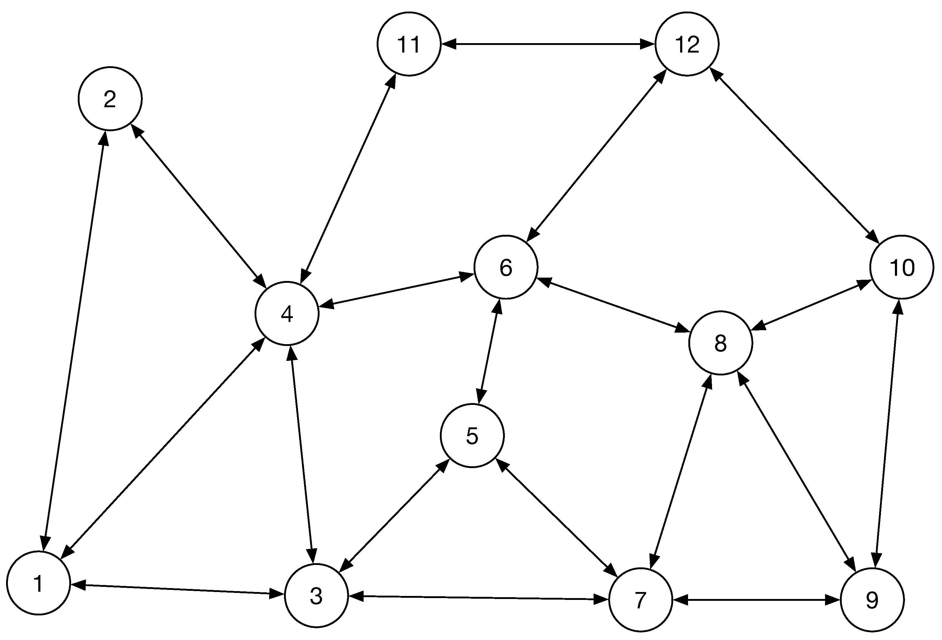
An evaluation of the system model previously presented in Section 3 is given for the network topology shown in Figure 2, whose links offer contact opportunities at an average rate of 1/200 contact/s. The links were defined as having identical channel rates of 800 Kbps and the same packet error rate values. The user workload consisted of 6 flows of 100 kB bundles sent at a designed rate (all at the same rate) whose value was an experimental factor. Table 1 shows details of the source and sink node numbers for each flow. While the test topology and the parameter values were arbitrarily chosen, the scenario included three main essential features found in complex space networks that were relevant to this study: the possibility of using multiple paths for data flows, each of limited availability, the presence of lossy channels, and network congestion occurring at different points due to shared use of links by the multi-hop paths. It is to be expected that other network topologies sharing these characteristics will show similar performance trends.
With the selected values, the nominal (error-free) average transmission time of a bundle over any link was . The one-way propagation delay of the links was defined as a second experimental factor. Two cases were studied.
4.1. Case 1: Homogeneous Network
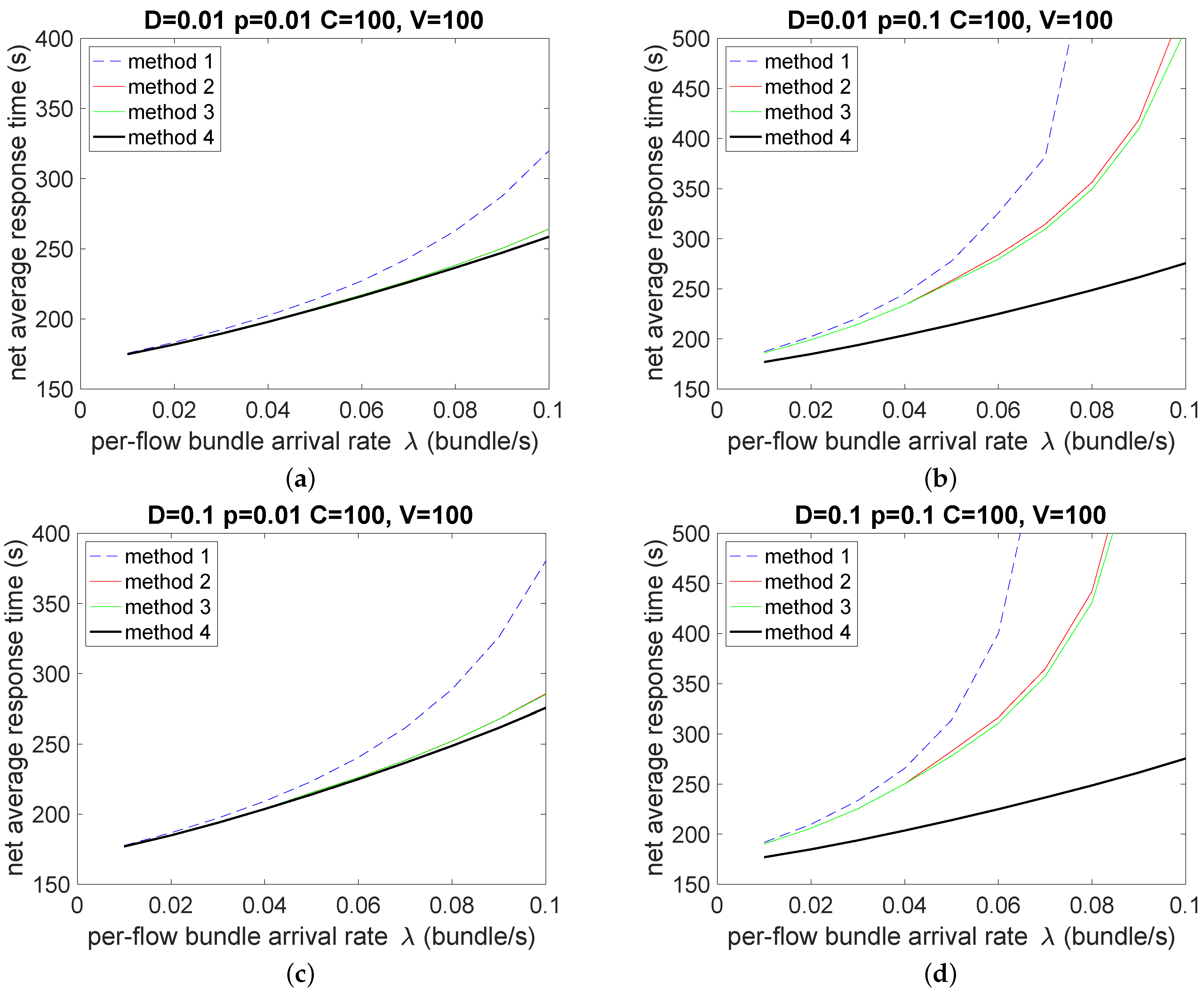
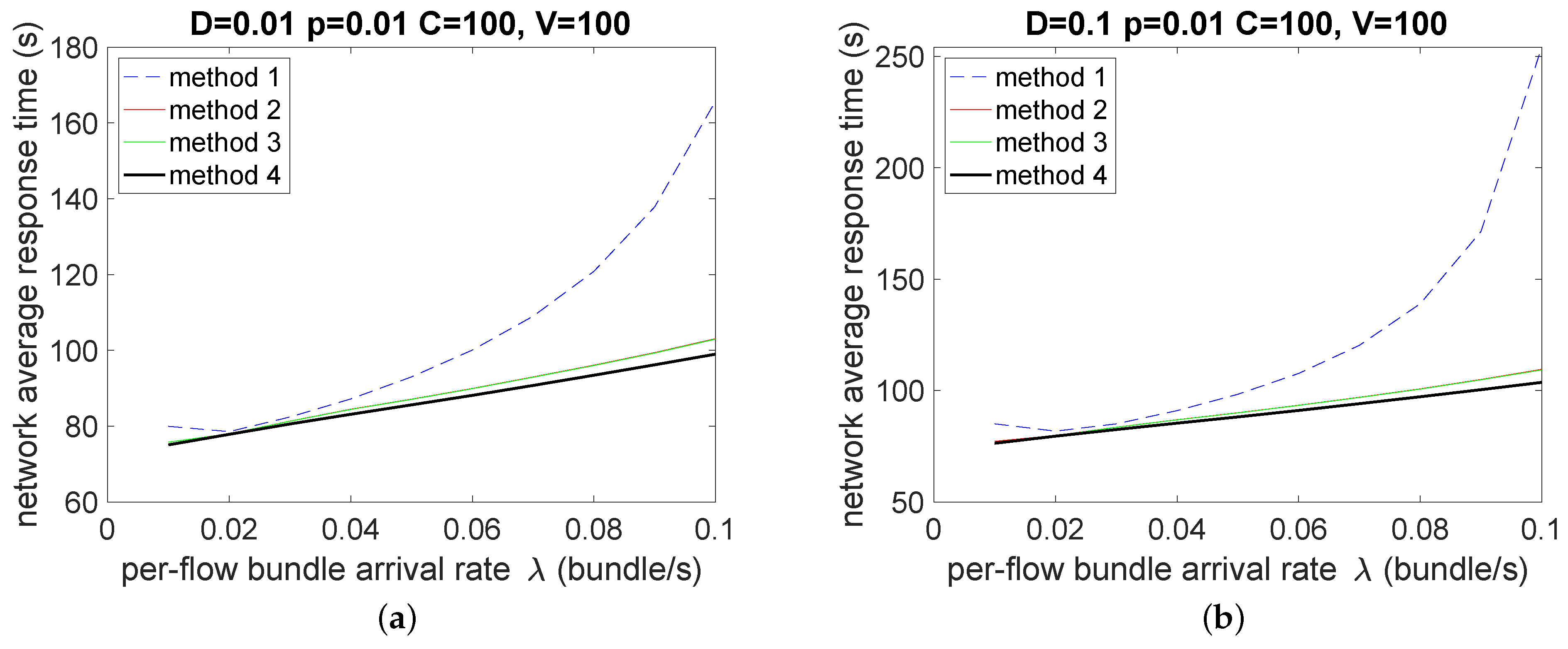
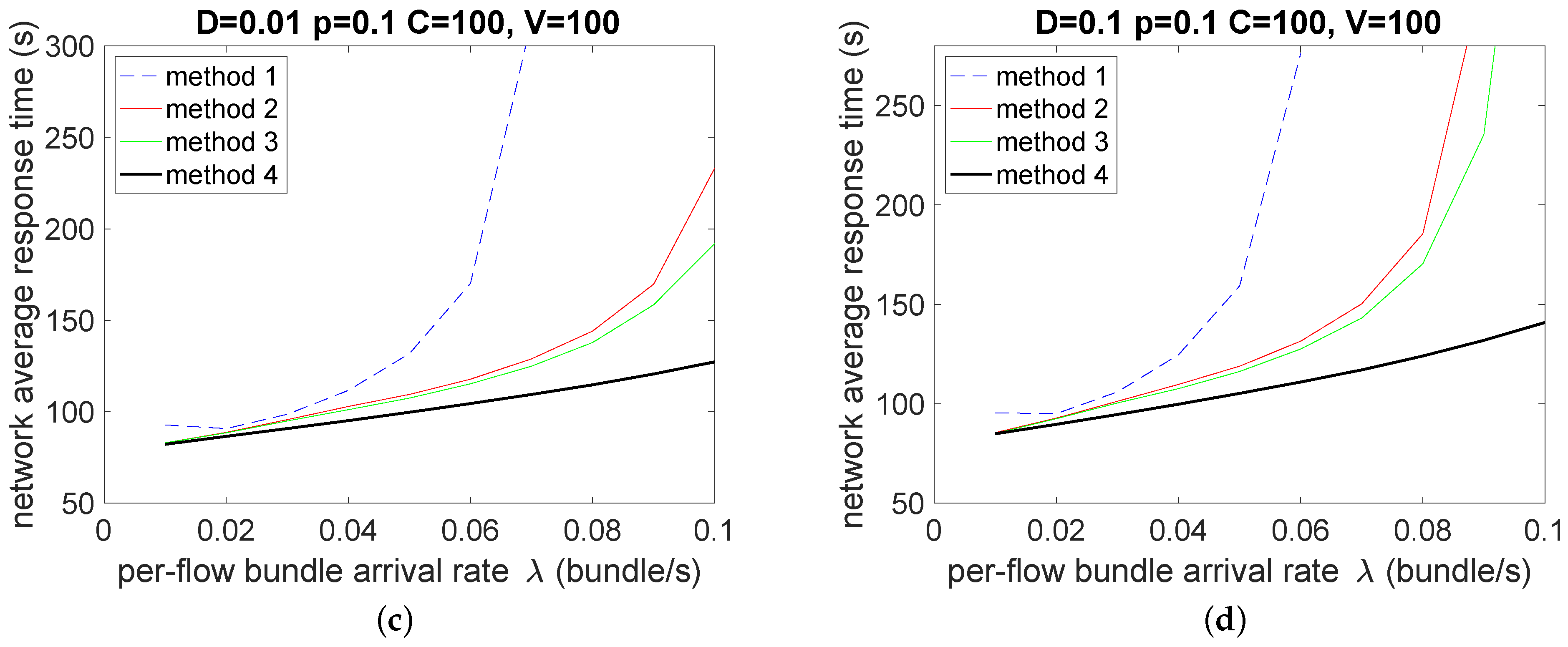
In the homogeneous case, all the network links were affected by the same average duration of 100 s for both link disruptions and contacts. Figure 3 depicts the network response time for four different cases. In Figure 3a, results for the case where both the one-way propagation delay and the packet loss ratio were fixed to 0.01. In Figure 3b, the one-way propagation delay was set to 0.01 but the packet loss ratio to 0.1. In Figure 3c these values were reversed. In Figure 3d, both the propagation delay and the packet loss ratio were fixed to 0.1.
The charts show the results for the average flow response time obtained by calculating the optimal flow routing using each of the four methods for the average service time as described in Section 3.5. The independent variable is the per flow sending rate. Because six flows were tested, the total arriving rate at the network was six times the value depicted in the figures. Given that the values of the propagation delays were selected to be smaller than the bundle transmission time, the sole use of the one-way propagation delay as an estimation of the service time led to response times significantly worse than the other three alternatives. Despite the inclusion of the bundle transmission time producing improvements to the average response time, no significant differences were observed between methods 2 and 3 (i.e., excluding or including the impact of the packet loss ratio), at least for the parameter values that were tested. The use of Equation (4) allowed achieving the lowest response time of the four methods for the entire range of flow rate values.
4.2. Performance Impact of the Packet Loss Ratio
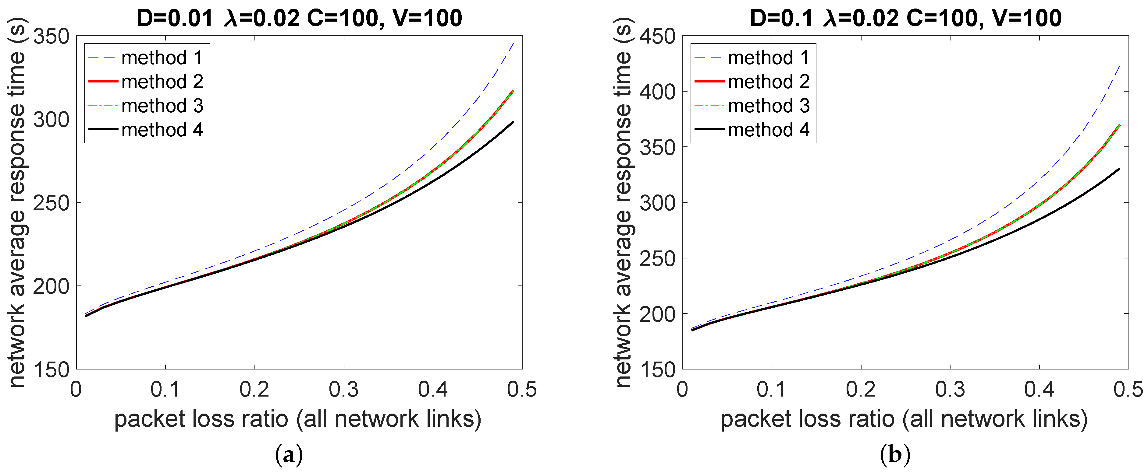
The impact on the flow routing performance of the packet loss ratio can be observed in Figure 4 for the four methods identified to calculate the bundle service time. The per flow bundle sending rate was fixed to a low value of , given that by increasing the packet loss ratio, the effective bundle service rate decreased. Cases for propagation delays of 0.01 s and 0.1 s are shown. The results indicate that increasing values for the packet loss ratio contributed to extending the gap between the performance of the service time methods. No significant difference between methods 2 and 3 was observed. The reason for this is that the disruption times (100 s) mainly drove the performance of the scenario rather than the service times of one second with method 2 and at most two seconds with method 3 (when ). Method 4 did produce noticeably lower response times for the worst transmission conditions.
4.3. Channel BER Deviations from the Contact Plan
While the current practice (i.e., ION-DTN CGR implementation) does not consider per contact BER values, in the possible case that BER values become associated with contacts for computing accurate bundle service times, underestimations are still possible, given that the expected BER values may be lower than the ones to be encountered when transmitting the bundle.
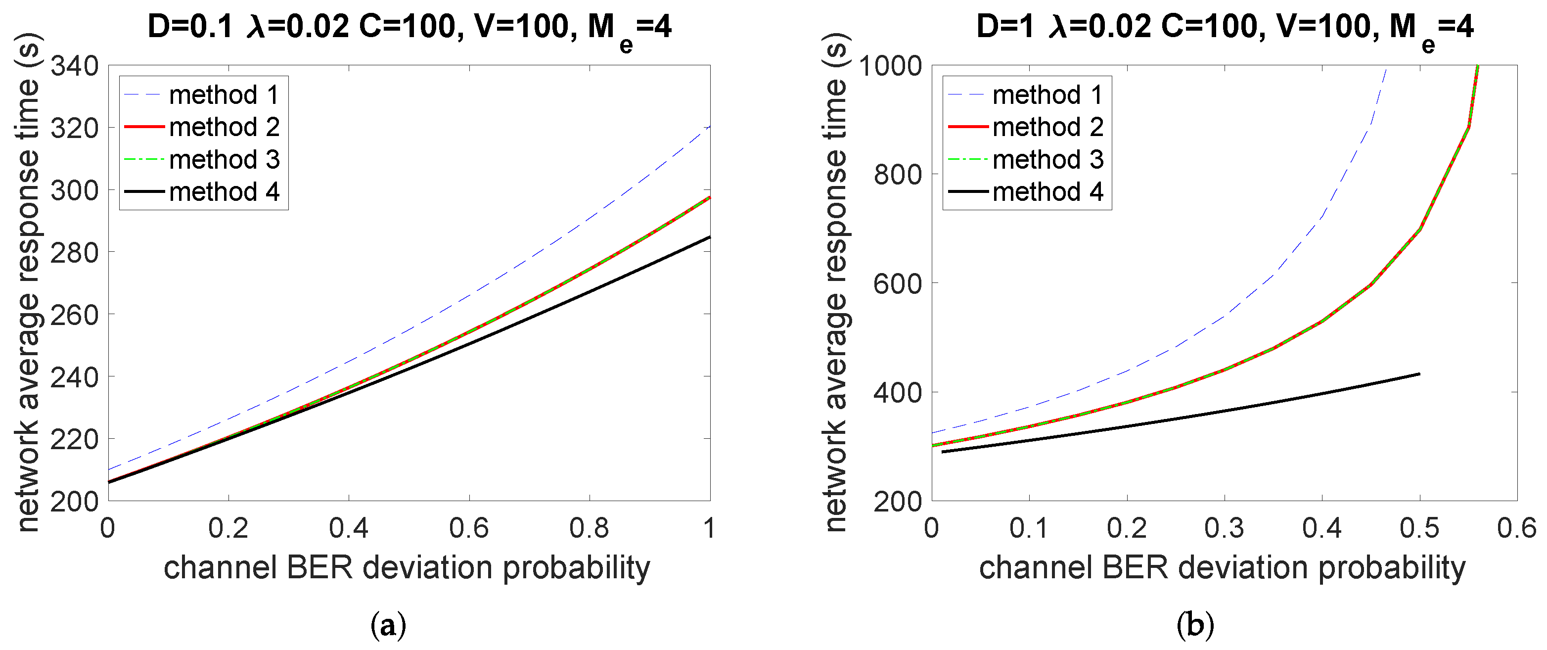
The impact of channel BER deviations from the plan is depicted in Figure 5 for two instances of 0.1 s and 1 s one-way propagation delay. The rest of the parameters were kept identical to the previous cases. To remove extra complexity in the presentation of the results, it was assumed that only one channel BER deviation may occur with a probability of . When that event happens, the effective BER for the bundle transmission increases by a factor of . The case depicted in Figure 5 assumes that . The numerical solution of the optimization problem shows that for small values for the propagation delay, the differences between methods 2–4 were minimal. Methods 2 and 3 performed almost identically for the same reasons given above. Larger propagation delays led to significant performance drops from the ideal performance.
4.4. Case 2: Heterogeneous Network
To observe the impact of heterogeneous link features, the average contact and disruption durations were randomly chosen for each link in the range to approximate the network average of the homogeneous case. To ensure evaluation fairness, the contact and disruption times were fixed to random values at the beginning of the evaluation, and the same values were used to evaluate all four service time estimation methods. Figure 6 depicts the results for the same parameter values that were used in the homogeneous network evaluation so that the results could be contrasted. While the overall trends were very similar to those observed before, the response times tended to be a bit lower than in the first evaluation case because of the specific random sample that was used. In that set, the average contact time was 351.75 s, and the average disruption time was 95.45 s, which offered a larger capacity than the homogeneous case with 100 s for both the contact and disruption periods, despite a lower contact rate of 0.0022 compared with 0.005 in the homogeneous case.
The results from both evaluation cases suggest that the current methods used for the estimation of the bundle transmission time in routing can yield large performance gaps compared with the suggested method. The next section evaluates the method with DTN protocols and a realistic test scenario.
5. Evaluation with DTN Protocols
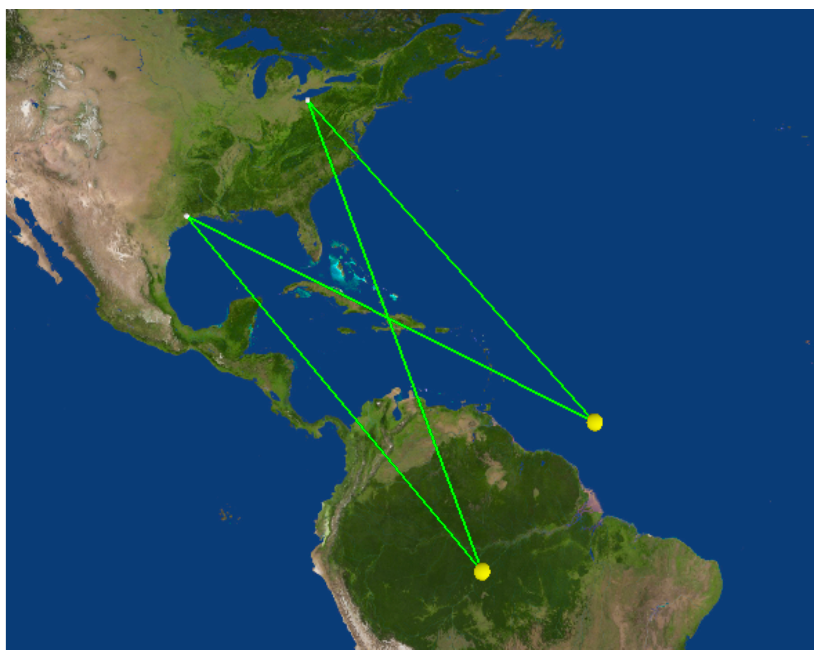
To verify the proposed method with specific DTN protocols and more realistic assumptions than the ones used in the prior section, consider the satellite transmission of data bundles between two locations from node g0, located near latitude 29.7604 and longitude −95.3698, and the destination node g1, located near latitude 41.4993 and longitude −81.6944, via two possible paths that become available periodically. This scenario is highly representative of a typical satellite communications scenario, where satellites are used as relays with multiple satellites within view that are able to provide the same service but only during certain time intervals. In this case, it is assumed that the operations center fixes the schedule that constrains the availability of each satellite for the intended test flow.
The network simulator defines an event-driven model of a queuing network that follows similar assumptions to the one used in the analysis: infinite queues for each outbound link and a first-come first-serve buffer serving policy. Figure 7 depicts the evaluation scenario. Both ground stations g0 and g1 and the satellites s0 and s1 are DTN nodes and therefore each capable of implementing store-carry-and-forward scheme. The satellites were assumed to be part of the tracking and data relay satellite (TDRS) constellation. Each satellite location was determined by the geosynchronous equatorial orbit (GEO) of TDRS-3 (s0) or TDRS-9 (s1) as given by the Skyfield library (https://rhodesmill.org/skyfield, accessed on 1 October 2022). The two-line element (TLE) set of the satellites was obtained from CelesTrak (https://celestrak.org/, accessed on 1 October 2022). The differences in the distance between the nodes produced slight variations in the propagation delay of up to approximately 7 ms, which made the path (g0, s1, g1) slightly faster than (g0, s2, g1). The propagation delay was calculated independently for each bundle at the start time of the transmission, as the wobbling effect of GEO satellites affected the propagation delay.
The test flow consisted of 200 bundles sent at a designated rate . Two cases were considered to better observe the influence of the service time. In the first case, the size of each bundle was 1 MB, and the transmission rate of all of the links was set to 1 Mbps. The links were scheduled to provide unaligned contacts of 100 s each every 1000 s; that is, the link disruptions did not occur in this case due to node mobility but because of link scheduling by mission control. The second case considered smaller bundles of 50 kB each and faster links of 10 Mbps, which cut the nominal radiation period by 200 times. To accelerate the simulations, the contact durations were shortened to 10 s every 100 s for each link. This reduced the realism but still allowed observing the relative performance improvement of the proposed method in a shorter time. In both cases, the downlink (s0, g1) was affected by controllable signal degradation, yielding a different channel BER than the other links. In addition, different tests were run for the flow sent from g0 to g1 and in the reverse direction.
The convergence layer adapter is given by the LTP, configured with a maximum block size equal to the bundle size so that a single LTP block is always needed for every bundle. The LTP implements retransmissions for reliability but is only allowed to retry a given block transmission for a certain number of times, given as a function of the expected channel BER. After that, the LTP drops the bundle. Additionally, the protocol was configured to not resume interrupted transmissions and instead drop the affected bundle, as the interest was in linking the benefits of the improved bundle transmission time estimation in terms of the bundle drop rate, which drove the network’s throughput. Routing was provided by CGR, either by using the original estimation method for the service time (i.e., Method 1) or the proposed approach (Method 4). It is important to note that CGR does not directly attempt to minimize the end-to-end bundle response times. Instead, the graph traversal method used by CGR has the approximated effect of finding the shortest contact path but with capacity considerations.
6. Results
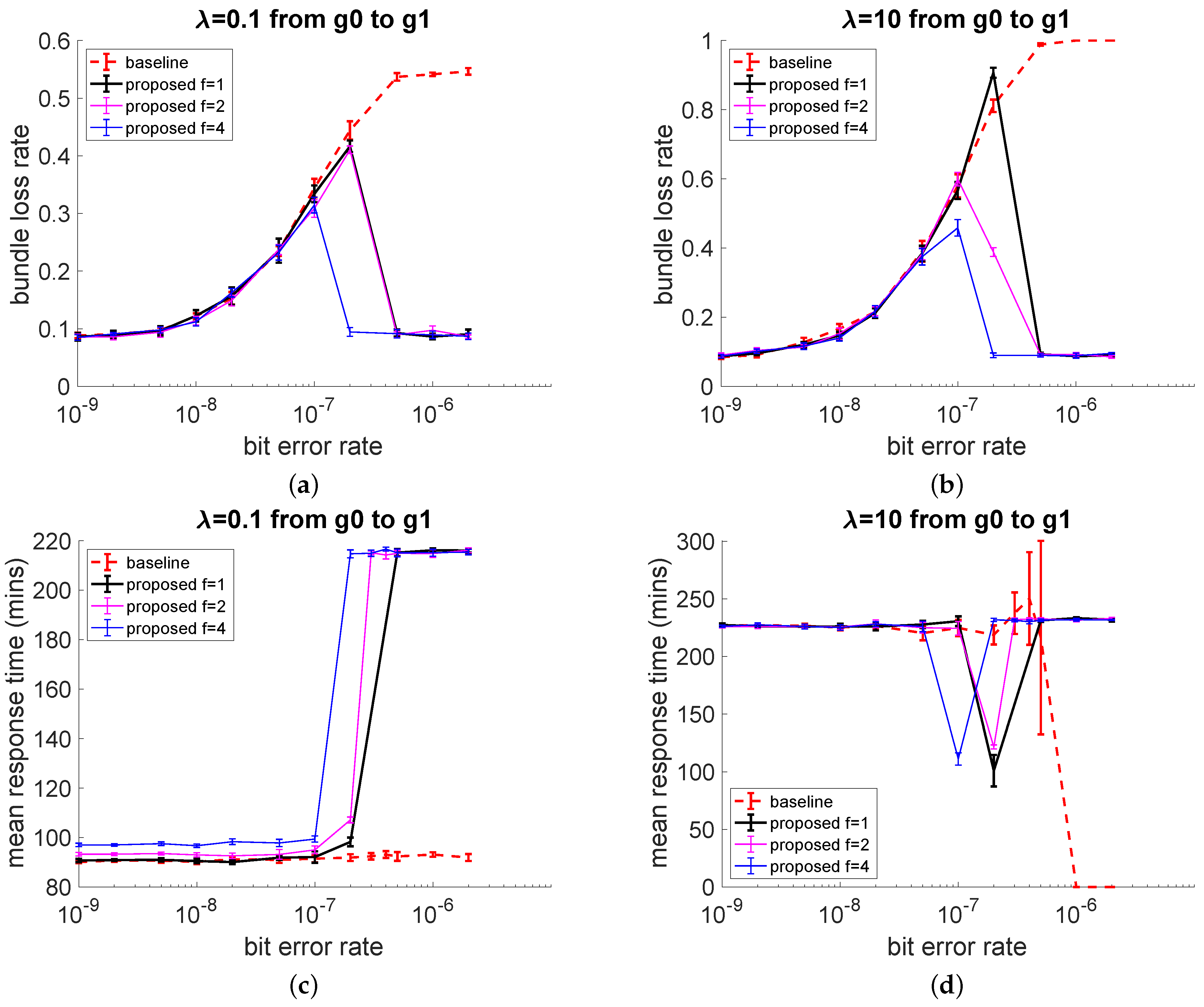
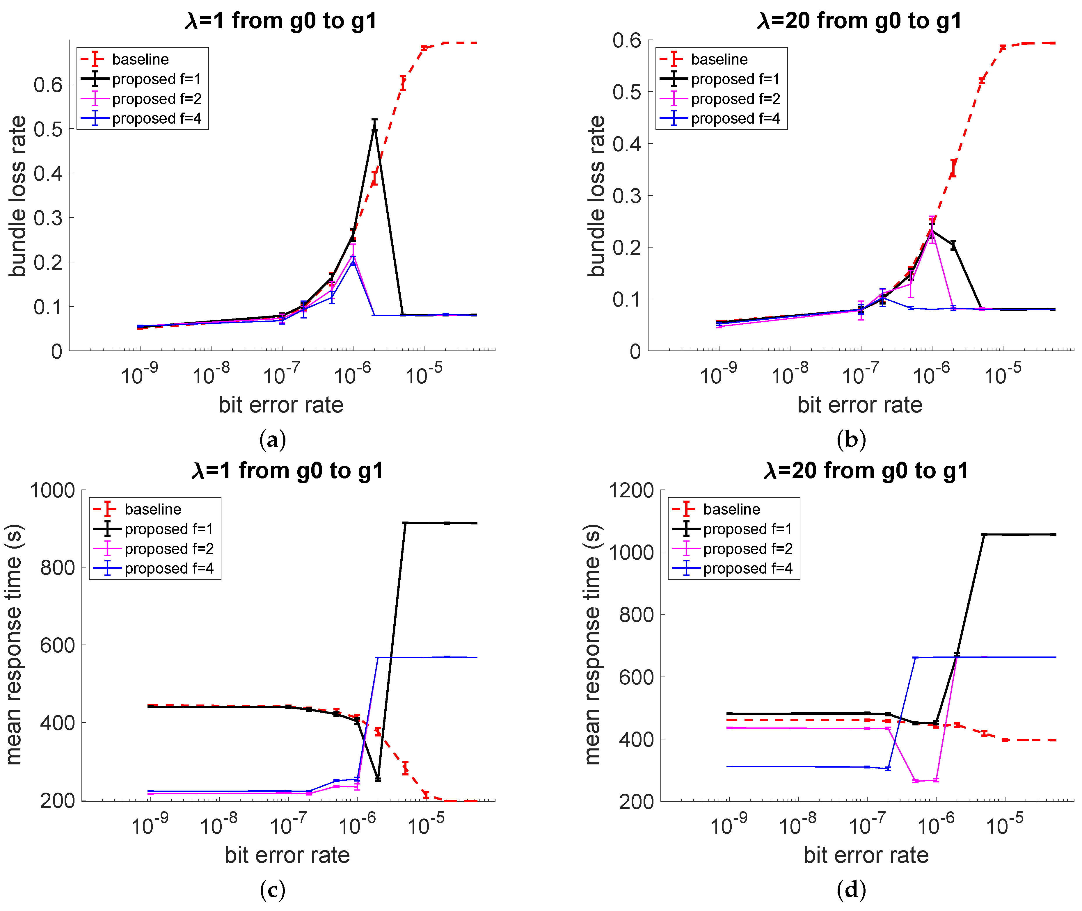
The average performance metrics for the first evaluation case are shown in Figure 8 for sending rates of 0.1 and 10 bundles/s from g0 to g1. The vertical bars indicate the 95% confidence interval. The baseline performance shown in red corresponds to method 2, with the bundle service time calculated without regard for the retransmission time, and this is the method implemented currently for CGR. The results for the improved service time estimation are shown for various values for parameter f (the multiplying factor for the service time estimation given by method 4). The channel BER, along with the LTP segment and block sizes, affects the bundle loss rate, but only the former was allowed to vary in this study. It can be observed that the bundle loss ratio exceeded 0.5 once the channel BER for the link (s0, g1) entered the 10 zone and continued growing with the current service time estimation method. The reported channel BER in this case was the value after the coding gain and therefore the BER that produced the segment losses. With the proposed improvement, it is feasible to continue operating with a low bundle loss ratio by allowing CGR switching to the second path. The response time metric aggregates the effective bundle transmission time (i.e., including retransmissions, and the buffering time).
The average bundle response time was observed to be higher with the improved method than with the standard one, and the reason for this behavior was that the heavy bundle losses experienced by the latter did not contribute to increasing the average response time. The fact that the average response time was higher with the proposed method shows that it allowed CGR to better decide how to switch paths. The results for the flow in the reverse direction (g1 to g0) are depicted in Figure 9. The performance was observed to be higher in this case, given that the higher-loss link was directly connected to the source for this test, allowing CGR to switch paths earlier in the path. In the prior case, after CGR decided to use s1, the next hop necessarily used the affected link, as it was not possible to return the bundle due to the split horizon mechanism for loop prevention.
Similar trends were observed for the second test case, but they occurred at a higher zone of BER values, given that the bundle sizes were reduced to 50 kB (see Figure 10 for the results for the g0 to g1 direction). Figure 11 shows the results for the reverse direction. As in the first case, the bundle loss rate continued to grow with the standard service time estimation method but was better controlled with the proposed method.
The use of actual DTN protocols in the evaluation and the resulting performance metrics from four test sets of different experimental conditions allowed making the following observations:
- The use of the proposed expression for the bundle service time helped CGR better identify the remaining volume of the contacts, yielding a better selection of the contact to be used for a bundle transmission for high BER values. No side effects were observed for low BER values, with the proposed service time expression achieving the same end-to-end performance as the standard.
- The complex interaction of DTN protocols and the stochastic behavior of the channel led to BER zones where the proposed method became less effective but still offered better performance than the standard method used by CGR. Interestingly, with very large BER values, it was easier for CGR to identify the contacts to be avoided. A larger hyperparameter allowed for reducing the gap in some cases.
- While the simulations assumed knowledge of the channel BER values, such knowledge may be replaced or complemented with measurements of the segment loss rate from the convergence layer adapter, given that the LTP uses a NACK mechanism to inform the sender engine what segments require retransmission.
7. Conclusions
In this work, an improved approximation for the bundle forwarding time with the LTP as the convergence layer (i.e., the link service time) was proposed for optimization of the bundle route selection in a space DTN. While it is reasonable to expect that the use of underestimated values for the service time will impact the routing performance, the quantification of such performance degradation is less evident. This study addressed this gap in the literature by conducting a stochastic modeling of a DTN with known statistical properties for the contact and duration times. The results have shown that solely using the propagation delay or the aggregation of the nominal service time (i.e., the expected one-hop delivery time over a lossless channel) and the link propagation delay, as performed in CGR, underestimates the bundle service time, which in turn leads to significant performance drops compared with the optimal levels. Moreover, the results have also shown that a geometric approximation of the extended bundle service time achieved by the reliable LTP is generally not sufficient to achieve the optimal routing performance. The tests with standard space DTN protocols demonstrated that the proposed service time expression for the bundle forwarding time can help CGR discover better paths for bundles. The channel BER is currently not used for routing nor included in the contact plan used by CGR. This study suggests that its inclusion and use of the proposed service time expression can lead to significant performance gains in a space DTN.
Funding
This work was supported by grant no. 80NSSC22K0259 from the National Aeronautics and Space Administration (NASA).
Conflicts of Interest
The author declares no conflict of interest.
Abbreviations
The following abbreviations are used in this manuscript:
| ARQ | Automatic repeat request |
| BER | Bit error rate |
| BP | Bundle protocol |
| CGR | Contact graph routing |
| CGR-ETO | CGR with earliest transmission opportunity |
| DTN | Delay- or disruption-tolerant network |
| GEO | Geosynchronous equatorial orbit |
| IPN | Interplanetary Internet |
| ION | Interplanetary Overlay Network |
| LTP | Licklider transmission protocol |
| NACK | Negative acknowledgment |
| NASA | National Aeronautics and Space Administration |
| SNR | Signal-to-noise ratio |
| TDRS | Tracking and data relay satellite |
| TLE | Two-line element |
References
- Burleigh, S.; Hooke, A.; Torgerson, L.; Fall, K.; Cerf, V.; Durst, B.; Scott, K.; Weiss, H. Delay-tolerant networking: An approach to interplanetary Internet. IEEE Commun. Mag. 2003, 41, 128–136. [Google Scholar] [CrossRef]
- Scott, K.; Burleigh, S.C. Bundle Protocol Specification. Internet Requests for Comments 5050, RFC Editor. 2007. Available online: https://doi.org/10.17487/RFC5050 (accessed on 1 October 2022).
- Araniti, G.; Bezirgiannidis, N.; Birrane, E.; Bisio, I.; Burleigh, S.; Caini, C.; Feldmann, M.; Marchese, M.; Segui, J.; Suzuki, K. Contact graph routing in DTN space networks: Overview, enhancements and performance. IEEE Commun. Mag. 2015, 53, 38–46. [Google Scholar] [CrossRef]
- The Interplanetary Overlay Network (ION) Software Distribution. ION-DTN. Available online: https://sourceforge.net/projects/ion-dtn (accessed on 1 October 2022).
- Lent, R. Analysis of the Block Delivery Time of the Licklider Transmission Protocol. IEEE Trans. Commun. 2019, 67, 518–526. [Google Scholar] [CrossRef] [PubMed]
- Scott, K.; Blanchet, M. Licklider Transmission Protocol (LTP), Compressed Bundle Header Encoding (CBHE), and Bundle Protocol IANA Registries. Internet Requests for Comments 7116, RFC Editor. 2014. Available online: https://doi.org/10.17487/RFC7116 (accessed on 1 October 2022).
- Bezirgiannidis, N.; Tsaoussidis, V. Packet size and DTN transport service: Evaluation on a DTN Testbed. In Proceedings of the International Congress on Ultra Modern Telecommunications and Control Systems, Moscow, Russia, 18–20 October 2010; pp. 1198–1205. [Google Scholar] [CrossRef]
- Lu, H.; Jiang, F.; Wu, J.; Chen, C.W. Performance improvement in DTNs by packet size optimization. IEEE Trans. Aerosp. Electron. Syst. 2015, 51, 2987–3000. [Google Scholar] [CrossRef]
- Alessi, N.; Burleigh, S.; Caini, C.; Cola, T.D. LTP robustness enhancements to cope with high losses on space channels. In Proceedings of the 2016 8th Advanced Satellite Multimedia Systems Conference and the 14th Signal Processing for Space Communications Workshop (ASMS/SPSC), Palma de Mallorca, Spain, 5–7 September 2016; pp. 1–6. [Google Scholar] [CrossRef]
- Shi, L.; Jiao, J.; Sabbagh, A.; Wang, R.; Yu, Q.; Hu, J.; Wang, H.; Burleigh, S.; Zhao, K. Integration of Reed-Solomon codes to licklider transmission protocol (LTP) for space DTN. IEEE Aerosp. Electron. Syst. Mag. 2017, 32, 48–55. [Google Scholar] [CrossRef]
- Wu, H.; Li, Y.; Jiao, J.; Cao, B.; Zhang, Q. LTP asynchronous accelerated retransmission strategy for deep space communications. In Proceedings of the 2016 IEEE International Conference on Wireless for Space and Extreme Environments (WiSEE), Aachen, Germany, 26–28 September 2016; pp. 99–104. [Google Scholar] [CrossRef]
- Wang, R.; Burleigh, S.C.; Parikh, P.; Lin, C.J.; Sun, B. Licklider Transmission Protocol (LTP)-based DTN for Cislunar Communications. IEEE/ACM Trans. Netw. 2011, 19, 359–368. [Google Scholar] [CrossRef]
- Wang, D. Performance of Licklider transmission protocol (LTP) in LEO-satellite communications with link disruptions. In Proceedings of the 2016 IEEE 15th International Conference on Cognitive Informatics Cognitive Computing (ICCI*CC), Palo Alto, CA, USA, 22–23 August 2016; pp. 154–159. [Google Scholar] [CrossRef]
- Acemoglu, D.; Johari, R.; Ozdaglar, A. Partially Optimal Routing. IEEE J. Sel. Areas Commun. 2007, 25, 1148–1160. [Google Scholar] [CrossRef]
- Hylton, A.; Short, R.; Green, R.; Toksoz-Exley, M. A Mathematical Analysis of an Example Delay Tolerant Network using the Theory of Sheaves. In Proceedings of the 2020 IEEE Aerospace Conference, Big Sky, MT, USA, 7–14 March 2020; pp. 1–11. [Google Scholar] [CrossRef]
- Bezirgiannidis, N.; Caini, C.; Montenero, D.P.; Ruggieri, M.; Tsaoussidis, V. Contact Graph Routing enhancements for delay tolerant space communications. In Proceedings of the 2014 7th Advanced Satellite Multimedia Systems Conference and the 13th Signal Processing for Space Communications Workshop (ASMS/SPSC), Livorno, Italy, 8–10 September 2014. [Google Scholar] [CrossRef]
- Segui, J.; Jennings, E.; Burleigh, S.C. Enhancing Contact Graph Routing for Delay Tolerant Space Networking. In Proceedings of the Global Communications Conference, GLOBECOM 2011, Houston, TX, USA, 5–9 December 2011; pp. 1–6. [Google Scholar] [CrossRef]
- Caini, C.; Fiore, V. Moon to Earth DTN communications through lunar relay satellites. In Proceedings of the 2012 6th Advanced Satellite Multimedia Systems Conference (ASMS) and 12th Signal Processing for Space Communications Workshop (SPSC), Vigo, Spain, 5–7 September 2012; pp. 89–95. [Google Scholar] [CrossRef]
- Yang, Z.; Wang, R.; Yu, Q.; Sun, X.; Sanctis, M.D.; Zhang, Q.; Hu, J.; Zhao, K. Analytical characterization of licklider transmission protocol (LTP) in cislunar communications. IEEE Trans. Aerosp. Electron. Syst. 2014, 50, 2019–2031. [Google Scholar] [CrossRef]
- Dudukovich, R.; LaFuente, B.; Hylton, A.; Tomko, B.; Follo, J. A Distributed Approach to High-Rate Delay Tolerant Networking within a Virtualized Environment. In Proceedings of the 2021 IEEE Cognitive Communications for Aerospace Applications Workshop (CCAAW), Cleveland, OH, USA, 21–23 June 2021; IEEE: Piscataway, NJ, USA, 2021. [Google Scholar] [CrossRef]
- Burleigh, S.; Caini, C.; Messina, J.J.; Rodolfi, M. Toward a unified routing framework for delay-tolerant networking. In Proceedings of the 2016 IEEE International Conference on Wireless for Space and Extreme Environments (WiSEE), Aachen, Germany, 26–28 September 2016; pp. 82–86. [Google Scholar]
- Marchese, M.; Patrone, F. E-CGR: Energy-Aware Contact Graph Routing Over Nanosatellite Networks. IEEE Trans. Green Commun. Netw. 2020, 4, 890–902. [Google Scholar] [CrossRef]
- De Jonckère, O.; Fraire, J.A. A shortest-path tree approach for routing in space networks. China Commun. 2020, 17, 52–66. [Google Scholar] [CrossRef]
- Ramadas, M.; Burleigh, S.; Farrell, S. Licklider Transmission Protocol—Specification; Internet Requests for Comments 5326, RFC Editor. 2008. Available online: https://doi.org/10.17487/RFC5326 (accessed on 1 October 2022).
- Yu, Q.; Burleigh, S.C.; Wang, R.; Zhao, K. Performance modeling of licklider transmission protocol (LTP) in deep-space communication. IEEE Trans. Aerosp. Electron. Syst. 2015, 51, 1609–1620. [Google Scholar] [CrossRef]
Figure 1.
Visual verification of the proposed simplified expression for the bundle service time compared to the complete model [5]. It is assumed there are a 100 kB bundle and block size, 1 Mbps channel rate, 1000 B payload, and 100 B headers. Results for one-way propagation delays of 0.1 s, 1 s, 10 s, and 100 s are presented.

Figure 2.
The evaluation network topology consisted of 12 nodes and 17 links. All of the links were subject to temporary but long-term disruptions, offering limited transmission opportunities between any two adjacent nodes.
Figure 2.
The evaluation network topology consisted of 12 nodes and 17 links. All of the links were subject to temporary but long-term disruptions, offering limited transmission opportunities between any two adjacent nodes.

Figure 3.
Average network response time as a function of the per flow sending rate of six concurrent flows obtained using four alternatives for estimating the one-hop bundle service time. Cases (a–d) show results for different comunication scenarios with a one-way propagation delay (D) and the packet loss ratio (p) set to either 0.1 or 0.01.

Figure 4.
Average network response time as a function of the packet loss ratio of (all) the links. With a higher chance of packet drops, the expected response time of the flow increases due to the additional transmission rounds needed for reliability. The differences from the ideal performance also become stronger. Cases with a one-way propagation delay of (a) or (b) are shown.

Figure 5.
Average network response time as a function of channel BER deviation probability. When a deviation occurrs, the BER increases four times, which extends service times and impacts the flow response times. Cases with a one-way propagation delay of (a) or (b) are shown.
Figure 5.
Average network response time as a function of channel BER deviation probability. When a deviation occurrs, the BER increases four times, which extends service times and impacts the flow response times. Cases with a one-way propagation delay of (a) or (b) are shown.

Figure 6.
Average response times on a heterogeneous network for four representative cases as a function of the per flow sending rate. In (a,c), the one-way propagation delay was , whereas in (b,d), . In (a,b) the packet loss ratio was whereas in (c,d), .
Figure 6.
Average response times on a heterogeneous network for four representative cases as a function of the per flow sending rate. In (a,c), the one-way propagation delay was , whereas in (b,d), . In (a,b) the packet loss ratio was whereas in (c,d), .


Figure 7.
Evaluation scenario. Two paths connect nodes g0 and g1 through TDRS-3 (s0) and TDRS-9 (s1).
Figure 7.
Evaluation scenario. Two paths connect nodes g0 and g1 through TDRS-3 (s0) and TDRS-9 (s1).

Figure 8.
Results for test case 1 with the traffic flowing from g0 to g1. The bundle loss ratio for a range of values of BER after the coding gain is shown for a bundle sending rate of (a) 0.1 bundle/s and (b) 10 bundles/s. The average bundle response time with the proposed method tended to be higher for larger BER values, given the queuing delay of the second path. Note that this outcome is not a weakness but is expected given the lower bundle loss. Charts (a,c) depict the results for a low sending rate . Results for a high sending rate are shown in (b,d).

Figure 9.
Results for test case 1 with the traffic flowing from g1 to g0 (reverse direction). Charts (a,c) depict the results with a light sending rate . Results for a high sending rate are shown in charts (b,d).
Figure 9.
Results for test case 1 with the traffic flowing from g1 to g0 (reverse direction). Charts (a,c) depict the results with a light sending rate . Results for a high sending rate are shown in charts (b,d).

Figure 10.
The results for test case 2 with the traffic flowing from g0 to g1, show a similar trend to case 1 but ocurring at a different zone of BER values. Charts (a,c) depict the case of light sending rates . The results for a high sending rate are shown in charts (b,d).
Figure 10.
The results for test case 2 with the traffic flowing from g0 to g1, show a similar trend to case 1 but ocurring at a different zone of BER values. Charts (a,c) depict the case of light sending rates . The results for a high sending rate are shown in charts (b,d).

Figure 11.
Bundle loss rate and mean response time results for test case 2 with the traffic flowing from g1 to g0 (reverse direction). Charts (a,c) depict the results with a light sending rate . Results for a high sending rate are shown in charts (b,d).
Figure 11.
Bundle loss rate and mean response time results for test case 2 with the traffic flowing from g1 to g0 (reverse direction). Charts (a,c) depict the results with a light sending rate . Results for a high sending rate are shown in charts (b,d).


Table 1.
The average network performance is given by the aggregated performance of six bundle flows in the evaluation study. The source-sink pairs were randomly selected and are indicated in this table.
Table 1.
The average network performance is given by the aggregated performance of six bundle flows in the evaluation study. The source-sink pairs were randomly selected and are indicated in this table.
| Flow ID | Source | Destination |
|---|---|---|
| 1 | 1 | 12 |
| 2 | 3 | 10 |
| 3 | 7 | 2 |
| 4 | 11 | 9 |
| 5 | 4 | 10 |
| 6 | 10 | 3 |
Disclaimer/Publisher’s Note: The statements, opinions and data contained in all publications are solely those of the individual author(s) and contributor(s) and not of MDPI and/or the editor(s). MDPI and/or the editor(s) disclaim responsibility for any injury to people or property resulting from any ideas, methods, instructions or products referred to in the content. |
© 2023 by the author. Licensee MDPI, Basel, Switzerland. This article is an open access article distributed under the terms and conditions of the Creative Commons Attribution (CC BY) license (https://creativecommons.org/licenses/by/4.0/).
Share and Cite
MDPI and ACS Style
Lent, R. Improving Bundle Routing in a Space DTN by Approximating the Transmission Time of the Reliable LTP. Network 2023, 3, 180-198. https://doi.org/10.3390/network3010009
AMA Style
Lent R. Improving Bundle Routing in a Space DTN by Approximating the Transmission Time of the Reliable LTP. Network. 2023; 3(1):180-198. https://doi.org/10.3390/network3010009
Chicago/Turabian StyleLent, Ricardo. 2023. "Improving Bundle Routing in a Space DTN by Approximating the Transmission Time of the Reliable LTP" Network 3, no. 1: 180-198. https://doi.org/10.3390/network3010009