

Detection of Malicious Network Flows with Low Preprocessing Overhead

Department of Computer Science, The University of Texas at San Antonio, San Antonio, TX 78249, USA
*
Author to whom correspondence should be addressed.
Network 2022, 2(4), 628-642; https://doi.org/10.3390/network2040036
Submission received: 12 August 2022
/
Revised: 27 October 2022
/
Accepted: 28 October 2022
/
Published: 4 November 2022
(This article belongs to the Special Issue Advanced Technologies in Network and Service Management)
Abstract
:Machine learning (ML) is frequently used to identify malicious traffic flows on a network. However, the requirement of complex preprocessing of network data to extract features or attributes of interest before applying the ML models restricts their use to offline analysis of previously captured network traffic to identify attacks that have already occurred. This paper applies machine learning analysis for network security with low preprocessing overhead. Raw network data are converted directly into bitmap files and processed through a Two-Dimensional Convolutional Neural Network (2D-CNN) model to identify malicious traffic. The model has high accuracy in detecting various malicious traffic flows, even zero-day attacks, based on testing with three open-source network traffic datasets. The overhead of preprocessing the network data before applying the 2D-CNN model is very low, making it suitable for on-the-fly network traffic analysis for malicious traffic flows.
1. Introduction
Network security tools utilize machine learning in various ways, but most machine learning implementations are computationally intensive. For this reason, analysis of large volumes of network traffic is traditionally reserved for a post-mortem or offline analysis of attacks. Machine learning solutions for live analysis are done only for a small fraction of the network traffic. However, by developing a machine learning approach that is comparatively simple while still maintaining high accuracy, that fraction may be increased, and it may even be possible to analyze each network flow in the network traffic.
Network traffic consists of different connections, called flows (defined by the 5-tuple of network protocol and the IP addresses and port numbers of both source and destination), between programs and services connected to the network. Each flow has one or more packets which contain the data being sent. One goal of network traffic analysis is to identify which flows consist of traffic from malicious programs, allowing those flows to be shut down or even prevented entirely. Therefore, it would be highly advantageous to analyze every flow in real time and with high malicious traffic detection accuracy.
Machine learning research is ongoing in various fields, but by far, the most researched forms of machine learning are those related to computer vision. For this reason, converting network traffic analysis, a traditionally non-visual task, to a computer vision task allows for more opportunities to apply novel and advanced analysis techniques to it. Convolutional Neural Networks (CNNs) are a relatively new form of machine learning model with various applications. Two-Dimensional CNNs (2D-CNNs), which take two-dimensional arrays of data such as pixels, are frequently used to analyze images for tasks such as object identification. Recently, several researchers have also used these models to analyze network traffic in a variety of ways [1,2,3,4,5,6,7].
Before analyzing using a machine learning model, the network traffic must generally undergo feature extraction. In feature extraction, features (attributes) that characterize different types of traffic need to be identified and, if necessary, calculated from the traffic, then compiled and packaged in a format suitable for machine learning model input. Examples of commonly used features include packets/second, connections/second, bytes/second, and packet header fields. This preprocessing of network traffic is a necessary time-consuming and resource-intensive step before applying an ML model to detect malicious flows.
Selecting the appropriate features is critical to the model’s performance and malicious flow detection accuracy. The set of essential features varies based on the network and traffic type that needs to be analyzed. Since it is hard to determine the essential features intuitively, it is common to start with a large number of features and select a smaller subset based on the analysis of each feature’s importance using specialized machine learning models or other approaches. Once the desired features are determined, the data corresponding to those features are extracted from the network packet capture (pcap) and converted to an appropriate format for input into the desired machine learning model.
Several research efforts in recent years have consisted of performing this feature extraction process to input the selected data into CNNs. However, an attractive trait of CNNs is that they can analyze raw data and identify noteworthy features quickly and efficiently. Therefore, CNNs are suited to object identification in images, with little or no image modification. The essential visual features are automatically determined and used by a CNN. Therefore, the computationally expensive task of identifying essential features and then extracting them during the data preprocessing stage of analysis may be unnecessary if a CNN is used to analyze the data. Several recent research efforts have focused on using One-Dimensional CNNs (1D-CNNs) to analyze network packets as a single one-dimensional array of bytes.
While these works are shown to detect malicious traffic accurately, the requirements of these techniques are too great. Their machine learning models are often complex. These models feature several convolution layers, each capable of being used as a stand-alone CNN similarly to the first layer in our model, which we will discuss in Section 3. They also have several large densely-connected layers, where every node in the layer is connected to every node in the layers before and after it. Moreover, their preprocessing methods are extensive, generally involving several conversions, calculations, and filters. Many of them also require a network flow to be completed before its features are extracted and analyzed. Owing to the high computational requirements, the current methods of detecting malicious traffic are more suitable for offline or post mortem analysis. Consequently, all of the analyses presented, which are based on post mortem analysis, are unsuitable for on-the-fly malicious flow detection.
The problem we address in this paper is to develop images from network traffic flows with very low overhead and apply deep learning (DL) models for image processing to detect anomalous flows. Specifically, we develop a simple method to convert raw IP (Internet Protocol) packet data directly into bitmap files and analyze with computer vision models such as the 2D-CNN without any significant preprocessing of the raw data. We evaluate our method’s effectiveness on three different network traffic datasets, including the popular USTC-TFC2016 dataset [1] used by numerous other research teams in this field of study, and we compare our results with those presented in the literature.
Our method has several advantages compared to 1D-CNN for raw packet analysis and 2D-CNN analysis based on extracted features or entire pcap file analysis. No extraneous analysis is required to identify what derived features are useful since all or a specified number of bytes of the packet are used for analysis. The 2D-CNN model then performs the work of identifying the useful features during model training; the trained model rapidly identifies anomalous traffic based on the chosen features of raw data.
Since our method uses the DL models developed for image analysis, any improvements in anomalous image detection are easily adapted for anomalous network traffic detection. For example, the research on 2D-CNN usage is ongoing and plentiful due to their visual applications, so there are a wide variety of different models to use for analysis. In contrast, the research into network security has focused mainly on 1D-CNN and other types of machine learning (ML) models. By efficiently converting packets into a format suitable analysis by the models used in visual machine learning tasks, any innovation in the field of computer vision may potentially be applied to network security, as well.
Furthermore, by using raw packet data instead of extracted features, our method allows for real-time traffic classification as soon as a new connection is initiated. In contrast, extraction of features requires collecting a minimum amount of network flow data before the analysis can begin. Therefore, our method uses fewer computational resources than any similar method that requires extracted features before applying a 2D-CNN model for analysis. Instead of storing and computing aggregate data, a necessary step for feature extraction, our method performs as few transformations on the raw packet data as possible before analyzing it. The binary data of a packet are simply appended to a predefined bitmap file header; no other changes need to be made.
Therefore, our methodology will likely be superior to the current malicious traffic detection methods. It allows for real-time analysis with less preprocessing overhead or specialized configuration and focuses on useful information to identify malicious flows. There is also a unique potential for further refinement by repurposing any advancement in computer vision research for use in this methodology.
The contributions we present in this paper are: (i) the proposal and demonstration of an efficient process for converting raw IP datagrams into bitmap images for analysis using DL models from computer vision research and (ii) a simple and effective deep learning model for computer vision capable of analyzing these images. We also (iii) test this method on several datasets. The first contribution is significant because it allows for accessible live malicious traffic detection using computer vision analysis. The second is an extension of the first that provides a practical deployment of the proposed network defense method. The third contribution demonstrates the effectiveness of this method and allows for comparison with other methods of live network defense.
The rest of this paper is structured as follows: Section 2 describes background of this research and related work, Section 3 describes the concept and design of our raw network analysis method, Section 4 outlines the implementation of our design, Section 5 reports the results of our initial experiments with this implementation, Section 6 discusses those results and their merits, and Section 7 summarily concludes the paper.
2. Background
Several researchers have used machine learning to analyze network traffic in ways similar to our proposed method. In this section we will review their techniques and identify how ours differs. First we will discuss researchers that have used similar data preprocessing techniques as ours to classify benign traffic data for network quality assurance. Then we will examine some malicious traffic detection techniques to use 1D-CNN to analyze streams of bytes from packets. Finally, we will discuss those who use 2D-CNN to analyze images generated from malicious packet data, whose techniques most closely resemble our own.
Xu et al. [7] produce images from 784 bytes of each IP datagram payload (transport layer segments) in the UNB ISCX VPN-nonVPN dataset [8] by treating each byte as an eight-bit integer grayscale pixel value. These images and their one-dimensional byte-stream counterparts are then used as input for an ensemble of parallel 2D-CNN, 1D-CNN, and RNN models. Weighted voting between these three models is used for the final classification of the traffic type.
Lim et al. [2] generate images by using four-bit segments of application layer packet data from the UPC dataset [9] as four-bit integer grayscale pixel values. A hybrid 2D-CNN+ResNet architecture is used to analyze these images and classify traffic based on application type.
These attempts to classify normal network traffic have produced promising results and high degrees of accuracy, but they have not attempted to identify malicious traffic types. However, they could potentially be adapted to a network security task. This could be done by adjusting the input and output parameters to accommodate other categories of labels, and training these models using labeled datasets containing malicious traffic as well as benign.
Marín et al. [3] use two different 1D-CNN models to analyze raw packet traces. Their first model is a complex multi-layer model that takes as input 1024 bytes of the first packet of each flow in the USTC-TFC2016 dataset [1]. This is shown to perform poorly (77% accuracy) compared to their second model, a simpler model using only one convolution layer that takes as input the first 100 bytes of the first two packets per flow, which can achieve nearly 100% accuracy on both the USTC-TFC2016 and CTU [10] datasets.
Zhang et al. [4] use the USTC-TFC2016 dataset [1] to analyze CPU usage of a 1D-CNN model while taking multiples of four bytes (between 54 and 784 bytes) from the first packet of each flow as input. They show that detection accuracy increases as more of a packet’s header is included, but CPU usage also increases relative to the number of bytes taken per packet. In order to identify a suitable balance between accuracy and CPU usage, they propose an implementation of their own CPU analysis to detect CPU utilization in deployment and adjust the window size accordingly.
Hwang et al. [5] examine the effects of using different numbers of bytes per packet and packets per flow as input for their 1D-CNN-based analysis on the USTC-TFC2016 [1] and Mirai-RGU [11] datasets using two 1D-CNN layers and seven densely-connected layers with between 10 and 1024 nodes in them. They take from each selected packet multiples of ten bytes, and a range from two to five packets per flow. They show that detection accuracy does not increase significantly by including more than two packets, and also show that including more of a packet’s header improves accuracy.
These 1D-CNN analysis methods are capable of achieving near-100% accuracy with the datasets used [1,10,11], but 2D-CNN is better suited to identifying initially unknown trends and relationships within the input data, depending on how the data are arranged within the image. Moreover, by necessitating input as images, it allows for a layer of abstraction from the original data. This may be a crucial first step towards opening an avenue for sharing packet-level attack data without compromising privacy.
Wang et al. [1] are the creators of the USTC-TFC2016 dataset used by several teams, including this one. They also generate .PNG image files by using the SplitCap tool to separate the dataset .pcap files into unidirectional flows or bidirectional sessions, and include either entire .pcap files or only application layer data. The first 784 bytes of the selected data are encoded into integers used to create pixel values. These images are then input into several types of 2D-CNN. Wang et al. show that the entire .pcap file containing flow data is best for analysis.
Zhang et al. [6] encode packet data into eight-bit integers in a zig-zag format in the corner of an image and then run a discrete cosine transform on the image. They then conduct analysis with a hybrid 2D-CNN and Deep Random Forest model based on the GoogLeNet model.
All of these techniques have produced near-100% detection accuracy, but they all rely on either extensive preprocessing methods, intricate multi-layer models with thousands of nodes, or both. Deep neural networks such as CNN are capable of running as standalone analysis tools without doing extraneous work to give them the answers, and even a small network can produce sufficiently high accuracy without as much computational effort.
Furthermore, several of these positive results rely heavily on the USTC-TFC2016 dataset, which does not have representative benign TCP flows. The benign traffic categories within this dataset contain virtually no samples of the traditional TCP connection sequence; the captured traffic in these categories is almost exclusively taken from connections that were already in progress at the start of the captures. Therefore, any published results that depend heavily on USTC dataset will need to be verified with more rigorous datasets.
We present a viable solution to real-time front-line threat detection based on the concept of minimal requirements. By focusing specifically on transport layer data and altering that data as little as possible except to add the file header necessary to label it an image, our model provides a promising starting point from which to develop an accurate, efficient detection tool.
3. Raw Network Traffic Analysis
Our goal is to create a front-line network security model capable of being used in real-time malicious flow identification with as little computing resources as possible, ideally allowing it to be run on individual switches in the data plane of a Software-Defined Network (SDN). Such an analysis would be well suited to deployment at the perimeter of an organizational network, but could effectively be deployed anywhere. This would not only be a powerful network security tool in its own right, but by requiring less computational resources than similar methods, it would be available to more network operators, thereby enhancing security across the Internet as a whole.
We are interested in ML/DL models that analyze meaningful raw bits (network and transport headers and their payloads) from network traffic and classify the flows as malicious or benign. The most commonly used ML models, such as RF, SVM, and k-NN [12,13], require extraction of features based on several packets of flows or the entire flows. Many DL models such as RNN and LSTM [13] also require feature extraction or aggregation of data over time. To avoid high processing overhead, we do not perform any elaborate feature extraction. We also avoid collecting data over time as much as possible to allow rapid detection. Other DL models such as autoencoders [13] can be used on individual samples of raw data and are suited to anomaly detection, but are not suited to detecting specific anomalies (such as malicious traffic) without carefully tailoring the training data to select portions that clearly demonstrate the anomalies, which is difficult to do broadly with raw packet data.
Neural networks such as Deep Neural Network (DNN) or 2D-CNN are designed to mimic neurological processes in biology, efficiently performing complex analysis of massive amounts of raw data. DNN would potentially be a valid model for our analysis as it can be used with either extracted features or raw data, but we seek to exploit advancements in image analysis techniques. Furthermore, prior research [14,15] indicates that DNN and CNN have similar training and detection speeds as well as detection accuracy when using similarly sized models and the same input features. 1D-CNN is also capable of analyzing raw data, but as we described in Section 2, 2D-CNN may be preferable for a number of reasons. Therefore, we focus on image processing models and converting traffic flows into images for analysis by 2D-CNN models.
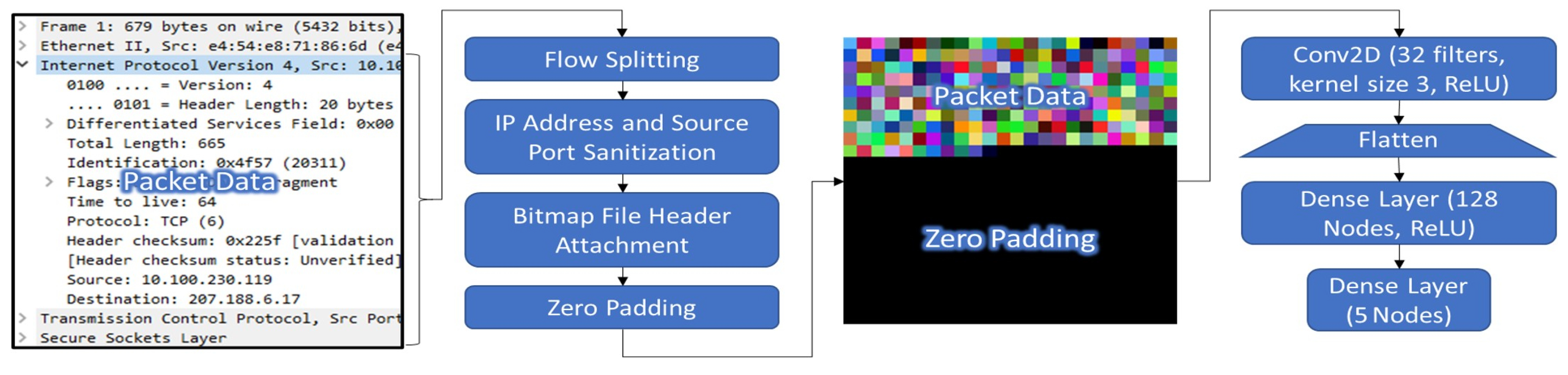
To accomplish our goal, we seek to perform as little processing as possible on the data. Therefore, rather than spending time on each flow waiting for enough data from which to extract features and performing the necessary calculations for feature extraction, we simply analyze the raw packet data directly. We extract the raw bits of IP datagrams from the first packet or two of a network flow and append those extracted bits to a pre-made bitmap file header to create a bitmap of the flow. We then use a simple 2D-CNN-based computer vision model to analyze the resulting bitmaps and classify them as either benign or malicious. The preprocessing steps and model are summarized in Figure 1.
3.1. Proposed Model
Our model consists of a single 2D-CNN layer of 32 filters with a kernel size of 3 and ReLU activation [16]. (Any negative values output by a neuron in the layer are adjusted to zero, and any positive values are simply output unchanged by the ReLU activation.) The configuration of the CNN layer means that 32 windows of 3 × 3 pixels shift across each bitmap to process it. The output of these filters on each section of the bitmap are then flattened into a single array suitable for input into a small densely-connected layer of 128 nodes, also with ReLU activation [16], in order to perform some analysis on the processed data from the CNN layer. This layer is then connected to a final densely-connected layer of 5 nodes; these predict the specific categories the model is meant to identify. The first two predict benign and malicious samples, respectively, while the remaining three consolidate any data which is not useful for the benign/malicious differentiation. The hyperparameters of this model are summarized in Table 1.

Table 1.
The hyperparameters of the 2D-CNN model. Any values not specified are left as the default settings for each layer.
Table 1.
The hyperparameters of the 2D-CNN model. Any values not specified are left as the default settings for each layer.
| 2D-CNN Model Details | |
|---|---|
| Layer | Hyperparameters |
| Conv2D | 32 filters, kernel size 3, ReLU |
| Flatten | N/A |
| Dense | 128 nodes, ReLU |
| Dense | 5 nodes |
The model works with bitmap images created from one or more packets per flow. The preprocessing complexity increases rapidly as more packets in a flow are used to create bitmaps. A table must be kept containing the first packet of each flow awaiting its second packet, methods of correlating each first packet to its second packet must be developed, protocols for dealing with a filled table must be defined, and a slew of security issues such as buffer overflows and denial of service attacks on this table need to be addressed. So any increase in detection accuracy must be balanced against the increase in the preprocessing complexity. In this paper, we consider two cases: images formed using the first packet of a flow and images formed using the first two packets of a flow.
By taking a limited number of packets from the beginning of a flow, the actual flow size and duration is irrelevant to detection speed or processing overhead. This type of analysis could inherently produce results faster than any analysis based on an entire flow, especially in cases where large volumes of data are passed through a single flow.
3.2. Early Flow Classification
One advantage of using only the first packet of a flow is simplicity. If no packets ever need to be correlated and analyzed together, the complexity of the required framework is greatly reduced. For example, for TCP flows, with one-packet images, only SYN packets need to be analyzed, which can be done without processing additional packets in that flow. Another advantage is that the time to detect a malicious flow is decreased. By beginning analysis upon receipt of the very first connection request, there is as little delay as possible from connection to identification. Waiting for additional packets also introduces additional delays, which may be crucial in cases of attacks where the damage done quickly, such as DDoS attacks, where the very act of connecting is the core of the attack.
One advantage of two-packet analysis is that malicious flow detection accuracy based on the first two packets can be significantly higher in some cases than that based on the first packet [3,5]. Our results also indicate that certain types of attacks are detected with a higher degree of accuracy when the second packet is included in analysis. For flows initiated by the external clients, the second packet of a flow is sent by an internal server quickly. Therefore, the additional wait time and the extra preprocessing overheads are not too high.
4. Methodology
In order to test the practicality of our design, we have produced a proof-of-concept working model which converts packet capture (.pcap) files to bitmap (.bmp) images and imports them into a 2D-CNN model designed in Keras [17], as shown in Figure 1.
4.1. Preprocessing
First, the .pcap files are processed to pseudo-randomize the IP addresses and source port numbers while preserving flows, which serves two functions. In small testbed-created datasets [1,18,19], one or very few internet IP addresses are used for attackers, which is not the likely scenario in botnet-based attacks. So, randomization of IP addresses eliminates the possibility that the detection is influenced by a small set of attacker IP addresses. Secondly, it may also be used to improve privacy in information sharing. In actual live detection, this randomization would not be needed for normal detection. However, if the bitmaps were to be shared so that other organizations could train their own models to defend against new attacks, our randomization step could serve as a layer of protection for the anonymity of private data that may be contained within.
Following address randomization, a script identifies each flow in each .pcap file, extracts the IP header and payload from the first n packets, where n is the number of packets being analyzed together from each flow, and appends them as-is to a bitmap file header. In this paper, n is 1 or 2.
4.2. Packets as Images
In order to convert raw packet data into bitmap images for 2D-CNN analysis, we extract individual packets from packet traces and append the IP payload of each packet to a predefined bitmap file header, which can be edited independently of the packet data to accommodate different bitmap features such as changing the image dimensions or color depth. Research into ideal bitmap formats is ongoing, but presently we use a 24-bit image of 24 pixels wide. Thus, each row of the image can store 72 bytes of data.
Due to the design specifications of the bitmap file format, image width must contain data in multiples of four bytes, but image height can be arbitrary. We leverage this to allow for the inclusion of several packets in the same image by tiling them vertically. This allows for packets in the same flow to be analyzed together by the model.
For the commonly used Ethernet frame payloads of 1500-byte packets, the bitmaps are thus 24 × 21 pixels (1512 bytes) for one packet, or 24 × 42 pixels for two packets. Any pixels not filled with packet data are set to all zeroes.
This method is particularly useful because the bitmap file header essentially provides a mapping to the pixel data. Any data can be appended to such a header, and it can be read as pixel data according to the specifications contained within the header. The data do not need to be processed in any way to allow for this conversion.
4.3. Model Implementation
The bitmap files, containing the specified number of packets from each flow in each packet trace, are then labeled as benign or malicious according to the published information provided with each dataset [1,18,19], and a random sample containing equal numbers of bitmaps from each of the categories in the data are used as input for the 2D-CNN model implemented in Keras for binary classification of malicious or benign flows.
We then use this Keras model to train on 90% of the selected bitmaps, and test on the other 10%, ensuring equal distribution from each category. We report results for ten epochs of training and testing.
This model is designed to be a simple representative of computer vision models as a class. This exact model architecture could be used to analyze a variety of input images for tasks such as reading handwritten characters. Thus, its performance should reflect the hypothetical performance of similar computer vision models.
4.4. Datasets
Our initial design has been tested on the USTC-TFC2016 (denoted USTC16) dataset used by several papers which analyze raw network traffic via different methods such as 1D-CNN [1,3,4,5]. This dataset contains ten categories of benign traffic and ten categories of malicious traffic, and at least 6000 flows in each category.
We also use the CIC-Denial-of-Service-2017 (CIC17) dataset [18] and the UTSA-2021-Low-rate-DoS-Attack (UTSA21) dataset [19]. The first dataset (CIC17) contains a benign category of mixed traffic, and eight categories of malicious traffic. The second (UTSA21) contains one benign category of HTTP traffic and two categories of low-rate Denial-of-Service attacks.
We take as many flows as we can from each category of traffic while ensuring that roughly equal numbers are taken, in order to ensure that each category is well-represented in the samples and balanced relative to the other categories. Balancing training is important because machine learning models often have higher classification accuracy when the training samples are balanced [20]. Thus, we also minimize the difference between the number of benign and malicious samples, to further ensure balanced training.
We then also combine these datasets, taking less from the categories containing larger quantities of samples, again so that each category is represented equally. We also limit the overall number of samples to avoid extending training time too much, as our goal is to create a model which can be used quickly and efficiently. Thus, when CIC17 is paired with either or both other datasets, we take fewer samples from each category of USTC16 and UTSA21, and when UTSA21 is paired with USTC16, we take fewer from the categories in the latter dataset. The number of samples used for each different combination are shown in Table 2.
These combinations are meant to create more diverse training and testing sets, allowing the model to analyze data which are more representative of the wide array of traffic occurring across the Internet.
4.5. Analysis Specifications
Each of these different analyses is run 30 separate times with different random seeds for sample selection, sample ordering, and model initialization, and the results of these 30 runs are averaged together to produce our final results for each case. This mimics the cross-validation commonly used in machine learning research [21]. The datasets used during each of the 30 runs in each analysis are available online [22].
This analysis is run using a 40-core Intel(R) Xeon(R) Gold 6230 CPU @ 2.10 GHz CPU and 256 GB of RAM. No GPU is used. During the course of analysis, the multi-threaded program utilizes on average 4 to 5 physical CPU cores (or 8–10 virtual cores).
We examine the results of our analyses using several different metrics: balanced accuracy, false negative rate, false positive rate, recall, precision, and F1 score [23].
Table 2.
The number of training and testing samples taken from each category in each dataset during each separate instance of analysis. Because the benign category of CIC17 contains mixed traffic, we take more from that benign category in all analyses. Specifically, we take 15,000 benign CIC17 samples for training, and 1500 for testing. Additionally, because of the imbalance in the number of benign and malicious categories in the UTSA21 dataset, we take twice as many benign samples for its individual analysis.
| Analysis Sample Selection | ||
|---|---|---|
| Dataset(s) | Training Samples per Category | Testing Samples per Category |
| USTC16 | 4800 | 1200 |
| UTSA21 | 3000 | 250 |
| CIC17 | 2000 | 150 |
| CIC+USTC | 1500 | 150 |
| CIC+UTSA | 2000 | 150 |
| USTC+UTSA | 2000 | 200 |
| CIC+USTC+UTSA | 1500 | 150 |
5. Results
In order to verify the efficacy of our design, we analyze the USTC16 dataset in two different scenarios. First, we examine a scenario in which the model is both trained and tested on all attacks, resembling the methods used in literature (Section 2). This allows us to compare our results to those of prior works directly. The second scenario consists of training the model using malicious flows from all but one category, and then testing on the remaining one, mimicking a ‘zero-day’ attack by treating the tested malicious category as a novel attack. This analysis has not been presented in prior literature referencing this dataset. However, it reflects an especially difficult case for the model to detect malicious traffic in live analysis, demonstrating its potential for real-world applications.
Our first analysis scenario consists of feeding a random sample of 6000 flows from each category into the model, using 90% of flows for training and 10% for testing. When using either one or two packets per flow, our model achieves greater than 99.95% testing balanced accuracy after ten epochs of training.
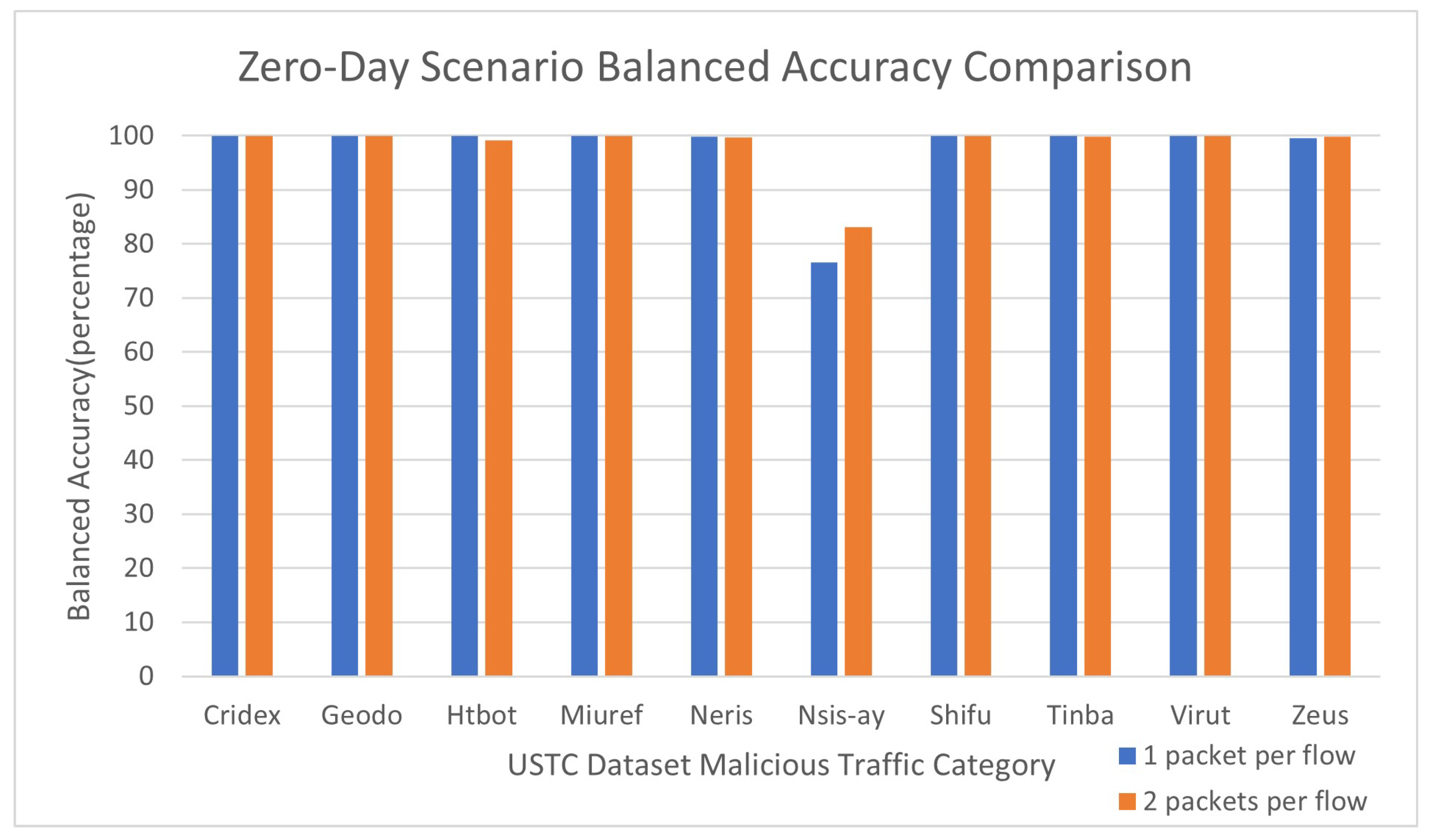
We then create a zero-day attack scenario in which the model encounters a new type of malicious traffic by only training on nine of the malicious categories, and testing on the remaining category separately. Our model performs extremely well (>99.5% balanced accuracy) using only one packet per flow against all malware categories except one (Nsis-ay). When using two packets per flow it performs better against Nsis-ay while also performing slightly worse against Htbot. All other categories are identified with nearly 100% recall and precision in either the 1-packet or 2-packet cases. These data are shown in Table 3. The balanced accuracy values are also shown in Figure 2.
In order to analyze the throughput of our model, we identify the training and testing times in each scenario of USTC analysis and calculate the flows processed per second while running experiments on the hardware described in Section 4. On average, for the one-packet case, training processes 2029 flows per second (fps) and testing 2258 fps. In the two packet scenario, training processes 1600 fps and testing 2286 fps.
This suggests that only training time is significantly affected by image size; the difference in testing time is not statistically significant. Since image size is directly based on how many bytes of a packet and packets per flow are analyzed, this implies that once a model is trained, there is no significant detriment to model throughput when using the full two packets suggested by prior research.
We then analyzed each of the three previously mentioned datasets alone and in tandem with each other, the results of which are summarized in Table 4. Analysis of only the USTC16 or UTSA21 datasets alone or combined with each other yields extremely high accuracy, but analyses including the CIC17 dataset show poorer detection rates and higher false positive and negative rates. However, analysis of two packets per flow performs better than one packet per flow in each of these cases.
Table 3.
An overview of the results of the simulated zero-day scenario using the USTC16 dataset.
| Zero-Day Scenario Results Overview | ||||||
|---|---|---|---|---|---|---|
| 1 Packet per Flow | 2 Packets per Flow | |||||
| Malware | Balanced Accuracy | Recall | Precision | Balanced Accuracy | Recall | Precision |
| Cridex | 100.0 | 100.0 | 100.0 | 100.0 | 100.0 | 99.9 |
| Geodo | 100.0 | 100.0 | 100.0 | 100.0 | 99.9 | 99.7 |
| Htbot | 100.0 | 100.0 | 100.0 | 99.2 | 98.4 | 100.0 |
| Miuref | 100.0 | 100.0 | 99.9 | 100.0 | 100.0 | 100.0 |
| Neris | 99.9 | 99.8 | 100.0 | 99.7 | 99.5 | 100.0 |
| Nsis-ay | 76.5 | 53.1 | 99.9 | 83.1 | 66.4 | 99.9 |
| Shifu | 100.0 | 100.0 | 100.0 | 99.9 | 99.9 | 100.0 |
| Tinba | 100.0 | 100.0 | 100.0 | 99.8 | 99.7 | 100.0 |
| Virut | 100.0 | 100.0 | 100.0 | 100.0 | 100.0 | 100.0 |
| Zeus | 99.5 | 99.1 | 100.0 | 99.9 | 99.8 | 100.0 |
6. Discussion
The results demonstrate that this method of flow analysis may be a powerful tool for network security. Considering that this is merely the first iteration of our design, with virtually no fine tuning, our design produces extremely promising results. This suggests that our proposed preprocessing method to utilize computer vision may be a viable method for malicious flow detection in live networks.
6.1. USTC16 Analysis
When analyzing the USTC16 dataset, the model achieves nearly 100% accuracy with only one packet per flow, demonstrating accuracy approximately equal to that of prior research.
Our model performed relatively poorly against the Nsis-ay category of malware, but prior methods which did report per-category performance also reported poor performance against one or more categories. Furthermore, the two-packet analysis demonstrated improved performance over the one-packet analysis. After investigating the Nsis-ay category manually, we determine that this category contains UDP flows which closely resemble the UDP traffic from several of the benign categories, such as Facetime and Skype.
However, we have found that even in most of these cases, most Nsis-ay flows have closer prediction values from the benign and malicious classifiers in the 5-node final layer of the model than those of the benign categories. These two prediction values are currently compared using a simple threshold; whichever value is higher is the prediction which is accepted. However, given that these values are generally very close for the Nsis-ay flows and generally not close for benign samples, adjusting this prediction threshold may be advantageous in future efforts. Analysis of this phenomenon suggests that a dynamic detection threshold may be able to increase accuracy to approximately 97% in the Nsis-ay category. Additionally, our two-packet analysis has already partially resolved the issue without any changes to the model.
6.2. USTC16 Results Comparison
A comparison of our proposed model with those of previous works which analyze the USTC16 dataset is shown in Table 5. Specifically, while our model demonstrates similar accuracy on the USTC16 dataset, it has lower complexity, less preprocessing, and is designed to be capable of live analysis. Additionally, since USTC16 proved to not be very challenging, the model has been tested on other publicly available datasets. These additional datasets also have a higher degree of attack diversity than those tested by some of the other prior works [3,5]. The additional datasets we used (CIC17 and UTSA21) featured a total of ten malicious categories, whereas the secondary datasets used by prior works only included two and eight categories, respectively.
The works which analyze USTC16 either have a much more complex and thus slower model [5], involve more in-depth preprocessing [1,3,4,5], or are inherently incapable of live detection prior to the end of a flow [1].
In [5], the model in question contains both a 1D-CNN layer with 32 filters of size 6 and another with 64 filters of size 6. This means that, despite using 1D-CNN, the CNN layers of their model are still approximately twice as large as the single CNN layer in ours. Their model also features seven consecutive densely-connected layers with a total of 3363 nodes within them, meaning over 800,000 connections between the dense layers, whereas our two small dense layers have only 640 connections between them.
In [1,3,4,5], extensive preprocessing is used to analyze the USTC16 dataset, involving multiple conversions and filters on the data such as changing the raw packet data into different number and vector formats, or performing several file conversion operations. Our model does not perform any such conversions, directly reading the raw packet data as pixel data instead.
In [1], the model presented can only achieve high accuracy when using entire pcap files containing all packets in completed flows as input to the model. Because our model only requires the first two packets of a flow, ours is able to begin analysis much faster.
Previous research [3] indicates that accuracy would improve when adding a second packet to analysis, but most of our USTC16 results do not reflect this. This may be because the prior research used different models for one- and two-packet analysis, whereas our model architecture is the same between the two cases. Furthermore, whenever the model does not achieve near-100% accuracy with one packet, two-packet analysis does improve detection accuracy. This can also be seen in the additional results in Table 4.
6.3. Analysis of CIC17 and UTSA21 Datasets
Our model has higher FPR and FNR when training and testing on the CIC-DoS-2017 dataset, where other researchers [14] have been able to achieve near-100% accuracy on this same dataset. However, our results are not directly comparable to the prior work, as our model uses only one or two packets per flow, while that work uses extracted features from entire flows. Despite this limited amount of data, our model is still able to detect malicious flows with over 90% accuracy after only one packet has been received.
Our results also resemble the near-100% accuracy of the previous work analyzing the UTSA21 dataset [19], but of the three models presented in that work, only one achieves that level of accuracy, and all of them require data collection over time and some form of feature extraction. All three of these models analyze various aspects of the timing of traffic (average inter-packet arrival time within each flow, inter-arrival time between new flows, and time slice data in windows of time), and thus must wait for a sufficient amount of temporal data before analysis can begin. Our analysis, however, is capable of beginning as soon as a single packet is received, as it is based on the raw characteristics of the packets themselves.
6.4. Confounding Factors
Confounding factors include the fact that within the USTC16 dataset used, most of the benign TCP traffic was captured from connections established prior to the start of the capture files. Thus, we are unable to adequately compare benign TCP connection requests with malicious TCP connection requests. The model is likely able to differentiate easily between the malicious traffic, which consists entirely of connection requests, and the benign traffic, which contains almost no connection requests. It is therefore possible that its high accuracy would not be reproducible on new packet traces where both malicious and benign categories contain TCP connection requests, though the same can be said of every other prior result that relies on the benign data in this dataset [1,3,4,5].
However, after analyzing other datasets, many cases still show high accuracy. This may indicate that these datasets also include some as-yet-unknown feature that allows the model to overtrain for them as well. However, it may also indicate that our model is indeed very useful for detecting malicious flows.
Our analysis has also thus far included packet payloads, which in our current dataset are unencrypted. We are unable to readily identify what features our model uses to classify flows due to the complexity of deep learning models. It is possible that one or more of the key features used by the model can be found within the payload of each packet, and encryption may obfuscate such features. Therefore, further testing is required to identify if the model could perform as well when considering encrypted traffic.
6.5. Live Analysis
To achieve our ultimate goal of live, real-time analysis, further work is required to fully automate the conversion of flows to bitmaps suitable for input into the model. This is done separately in our current tests, but can be easily automated and streamlined to allow for real-time conversion.
Real-time analysis would also require us to develop a means of reliably extracting at least the first packet from each flow. In order to do this, we intend to use the features of Software-Defined Networking (SDN) [24] which allow packets to be copied and forwarded to different sources based on configurable flow rules.
Additionally, though we only test IPv4 in this work, it would be advantageous for live implementation to also include support for IPv6. The model itself could be easily extended to IPv6, as the structure of IPv4 and IPv6 packets is similar in many respects.
7. Conclusions
In this paper, we have presented a novel form of network traffic analysis which consists of rapidly converting data packets directly into bitmap images suitable for visual machine learning analysis models. We then used a popular form of image classification model, the Two-Dimensional Convolutional Neural Network, to analyze these bitmap images, demonstrating comparable accuracy on a variety of datasets to the models reported in related work. This suggests that our method, which is computationally simpler and requires less preprocessing and lower data collection delays than the prior methods, is more suited to real-time analysis.
We still need to demonstrate that it is efficient enough to use for real-time analysis. To do this, we will need to do more thorough testing to identify the run time, throughput, and computational overhead. This will also require some refinements to the preprocessing steps, and a method of extracting packets directly from live network traffic instead of merely from .pcap files.
Additionally, further research into training and testing this analysis method on more datasets and training and testing between datasets is ongoing.
While further research into the practicality and portability of this technique is required, initial results indicate that this may become an important tool for automating network traffic analysis.
Author Contributions
G.F.’s contributions include design and implementation of the model used in this study, analyses of the datasets, and writing the paper. R.V.B.’s contributions include the initial ideas, selection of datasets, evaluation of the analysis results, and writing the paper. All authors have read and agreed to the published version of the manuscript.
Funding
This research was partially supported by grants from the US National Security Agency under contracts H98230-20-1-0392 and H98230-21-1-0171.
Institutional Review Board Statement
Not applicable.
Informed Consent Statement
Not applicable.
Data Availability Statement
Publicly available datasets were analyzed in this study. The sources are cited in the paper. The processed versions of these datasets by the authors were published on Harvard Dataverse and cited in the paper: https://doi.org/10.7910/DVN/O5A0ZV (accessed on 12 August 2022).
Acknowledgments
The opinions expressed and any errors contained in the paper are those of the authors. This paper is not meant to represent the position or opinions of the authors’ institution or the funding agencies.
Conflicts of Interest
The authors declare no conflict of interest.
References
- Wang, W.; Zhu, M.; Zeng, X.; Ye, X.; Sheng, Y. Malware traffic classification using convolutional neural network for representation learning. In Proceedings of the 2017 International Conference on Information Networking (ICOIN), Da Nang, Vietnam, 11–13 January 2017; pp. 712–717. [Google Scholar] [CrossRef]
- Lim, H.K.; Kim, J.B.; Heo, J.S.; Kim, K.; Hong, Y.G.; Han, Y.H. Packet-based Network Traffic Classification Using Deep Learning. In Proceedings of the 2019 International Conference on Artificial Intelligence in Information and Communication (ICAIIC), Okinawa, Japan, 11–13 February 2019; pp. 46–51. [Google Scholar] [CrossRef]
- Marín, G.; Casas, P.; Capdehourat, G. DeepMAL—Deep Learning Models for Malware Traffic Detection and Classification. arXiv 2020, arXiv:2003.04079. [Google Scholar]
- Zhang, W.; Wang, J.; Chen, S.; Qi, H.; Li, K. A Framework for Resource-aware Online Traffic Classification Using CNN. In Proceedings of the 14th International Conference on Future Internet Technologies, Phuket, Thailand, 7–9 August 2019; pp. 1–6. [Google Scholar] [CrossRef]
- Hwang, R.H.; Peng, M.C.; Huang, C.W.; Lin, P.C.; Nguyen, V.L. An Unsupervised Deep Learning Model for Early Network Traffic Anomaly Detection. IEEE Access 2020, 8, 30387–30399. [Google Scholar] [CrossRef]
- Zhang, X.; Chen, J.; Zhou, Y.; Han, L.; Lin, J. A Multiple-Layer Representation Learning Model for Network-Based Attack Detection. IEEE Access 2019, 7, 91992–92008. [Google Scholar] [CrossRef]
- Xu, L.; Zhou, X.; Ren, Y.; Qin, Y. A Traffic Classification Method Based on Packet Transport Layer Payload by Ensemble Learning. In Proceedings of the 2019 IEEE Symposium on Computers and Communications (ISCC), Barcelona, Spain, 29 June–3 July 2019; pp. 1–6. [Google Scholar] [CrossRef]
- Draper-Gil, G.; Lashkari, A.H.; Mamun, M.S.I.; Ghorbani, A.A. Characterization of Encrypted and VPN Traffic using Time-related Features. In Proceedings of the 2nd International Conference on Information Systems Security and Privacy (ICISSP), Rome, Italy, 19–21 February 2016; pp. 407–414. [Google Scholar] [CrossRef]
- Carela-Español, V.; Bujlow, T.; Barlet-Ros, P. Is our ground-truth for traffic classification reliable? In Proceedings of the 2014 International Conference on Passive and Active Network Measurement, Los Angeles, CA, USA, 10–11 March 2014; Springer: Berlin/Heidelberg, Germany, 2014; pp. 98–108. [Google Scholar] [CrossRef]
- Garcia, S.; Grill, M.; Stiborek, J.; Zunino, A.; Vedula, V.; Lama, P.; Boppana, R.V.; Trejo, L.A. An empirical comparison of botnet detection methods. Comput. Secur. 2014, 45, 100–123. [Google Scholar] [CrossRef]
- McDermott, C.D.; Majdani, F.; Petrovski, A.V. Botnet detection in the internet of things using deep learning approaches. In Proceedings of the 2018 International Joint Conference on Neural Networks (IJCNN), Rio de Janeiro, Brazil, 8–13 July 2018; pp. 1–8. [Google Scholar] [CrossRef]
- Ray, S. Commonly Used Machine Learning Algorithms (with Python and R Codes). 2017. Available online: https://www.analyticsvidhya.com/blog/2017/09/common-machine-learning-algorithms/ (accessed on 3 February 2022).
- Brownlee, J. A Tour of Machine Learning Algorithms. 2019. Available online: https://machinelearningmastery.com/a-tour-of-machine-learning-algorithms/ (accessed on 3 February 2022).
- Yungaicela-Naula, N.M.; Vargas-Rosales, C.; Perez-Diaz, J.A. SDN-Based Architecture for Transport and Application Layer DDoS Attack Detection by Using Machine and Deep Learning. IEEE Access 2021, 9, 108495–108512. [Google Scholar] [CrossRef]
- Zhang, Y.; Chen, X.; Guo, D.; Song, M.; Teng, Y.; Wang, X. PCCN: Parallel Cross Convolutional Neural Network for Abnormal Network Traffic Flows Detection in Multi-Class Imbalanced Network Traffic Flows. IEEE Access 2019, 7, 119904–119916. [Google Scholar] [CrossRef]
- Brownlee, J. A Gentle Introduction to the Rectified Linear Unit (ReLU). 2019. Available online: https://machinelearningmastery.com/rectified-linear-activation-function-for-deep-learning-neural-networks/ (accessed on 3 February 2022).
- Chollet, F. Keras; Github: San Francisco, CA, USA, 2015; Available online: https://github.com/fchollet/keras (accessed on 22 September 2022).
- Jazi, H.H.; Gonzalez, H.; Stakhanova, N.; Ghorbani, A.A. Detecting HTTP-based application layer DoS attacks on web servers in the presence of sampling. Comput. Netw. 2017, 121, 25–36. [Google Scholar] [CrossRef]
- Vedula, V.; Lama, P.; Boppana, R.V.; Trejo, L.A. On the Detection of Low-Rate Denial of Service Attacks at Transport and Application Layers. Electronics 2021, 10, 2105. [Google Scholar] [CrossRef]
- Wei, Q.; Dunbrack, R.L., Jr. The role of balanced training and testing data sets for binary classifiers in bioinformatics. PLoS ONE 2013, 8, e67863. [Google Scholar] [CrossRef] [Green Version]
- Cross-Validation (Statistics): Repeated Random Sub-Sampling Validation. 2022. Available online: https://en.wikipedia.org/wiki/Cross-validation_(statistics)#Repeated_random_sub-sampling_validation (accessed on 3 February 2022).
- Fox, G.; Boppana, R.V. Replication Data for: Detection of Malicious Network Flows with Low Preprocessing Overhead. Harv. Dataverse 2022. [Google Scholar] [CrossRef]
- Precision and Recall: Definition (Classification Context). 2022. Available online: https://en.wikipedia.org/wiki/Precision_and_recall#Definition_(classification_context) (accessed on 3 February 2022).
- Kirkpatrick, K. Software-defined networking. Commun. ACM 2013, 56, 16–19. [Google Scholar] [CrossRef]
Figure 1.
The full data pipeline for our analysis. The first half show preprocessing done on PCAP (network traffic) files to produce separate BMP (bitmap image) files for each flow. IP addresses in each bidirectional flow are randomized to create the effect of multiple attack sources. The IP datagrams from each flow are extracted and appended as-is to a predefined BMP file header. The second half shows the 2D-CNN model used for processing, including information about each layer. This information is also shown in Table 1. The packet data show the pipeline for a single packet; in two-packet analysis, the image would be twice the height, with the other half containing the second packet’s data.

Figure 2.
Balanced accuracy of simulated zero-day scenario, training for ten epochs on nine malicious categories from USTC-TFC2016 dataset and testing on the tenth while taking 6000 flows from each benign category in a 90%/10% split for training and testing. All scenarios except testing on Nsis-ay are near 100% balanced accuracy after ten epochs of training.

Table 4.
An overview of the results from training and testing on equal amounts from each category in each of the three datasets in various combinations as listed in Table 2. In general, any case containing CIC-DoS17 traffic demonstrates lower accuracy, but every case not containing that traffic has nearly 100% accuracy.
| Results Overview (1 Packet per Flow) | ||||||
|---|---|---|---|---|---|---|
| Datasets | Balanced Accuracy | Recall | Precision | FNR | FPR | F1 Score |
| CIC17 | 90.6 | 84.3 | 95.6 | 15.7 | 3.2 | 89.6 |
| USTC16 | 100.0 | 100.0 | 100.0 | 0.0 | 0.0 | 100.0 |
| UTSA21 | 100.0 | 100.0 | 100.0 | 0.0 | 0.0 | 100.0 |
| CIC17+USTC16 | 88.4 | 90.0 | 86.5 | 10.0 | 13.1 | 88.2 |
| CIC17+UTSA21 | 91.8 | 87.6 | 95.3 | 12.4 | 4.0 | 91.3 |
| USTC16+UTSA21 | 99.8 | 99.7 | 99.9 | 0.3 | 0.1 | 99.8 |
| CIC16+USTC16+UTSA21 | 89.2 | 93.8 | 85.5 | 6.2 | 15.5 | 89.4 |
| Results Overview (2 Packets per Flow) | ||||||
| Datasets | Balanced Accuracy | Recall | Precision | FNR | FPR | F1 Score |
| CIC17 | 93.2 | 90.8 | 94.4 | 9.2 | 4.4 | 92.6 |
| USTC16 | 100.0 | 99.9 | 100.0 | 0.1 | 0.0 | 100.0 |
| UTSA21 | 100.0 | 100.0 | 100.0 | 0.0 | 0.0 | 100.0 |
| CIC17+USTC16 | 95.3 | 94.0 | 96.2 | 6.0 | 3.4 | 95.1 |
| CIC17+UTSA21 | 94.2 | 92.5 | 95.6 | 7.5 | 4.0 | 94.0 |
| USTC16+UTSA21 | 99.9 | 99.8 | 99.9 | 0.2 | 0.1 | 99.9 |
| CIC16+USTC16+UTSA21 | 95.4 | 94.7 | 96.0 | 5.3 | 3.8 | 95.3 |
Table 5.
A comparison of our proposed model with related works using the USTC16 dataset. All works presented achieve approximately 100% balanced accuracy when analyzing this dataset alone. Model Complexity is reported as a measure of number of layers. The Live column indicates whether the proposed solution’s design allows for live analysis prior to the end of a flow.
| Paper | Models Used | Packets per Flow | Packet Types and Formats | Model Complexity | Live | Datasets Analyzed |
|---|---|---|---|---|---|---|
| This Paper | 2D-CNN | First 2 | Raw IP datagrams | 4 | Yes | CIC17 [18], USTC16 [1], UTSA21 [19] |
| Wang et al. [1] | 2D-CNN | All | Entire pcap files | 7 | No | USTC16 [1] |
| Marín et al. [3] | 1D-CNN | First 2 | Raw packets in pcap files | 5 | Yes | USTC16 [1], CTU [10] |
| Zhang et al. [4] | 1D-CNN | First 1 | Raw packets in pcap files | 14 | Yes | USTC16 [1] |
| Hwang et al. [5] | 1D-CNN + Auto-encoder | First 2 | Raw packets in pcap files | 11 | Yes | USTC16 [1], Mirai-RGU [11] |
Publisher’s Note: MDPI stays neutral with regard to jurisdictional claims in published maps and institutional affiliations. |
© 2022 by the authors. Licensee MDPI, Basel, Switzerland. This article is an open access article distributed under the terms and conditions of the Creative Commons Attribution (CC BY) license (https://creativecommons.org/licenses/by/4.0/).
Share and Cite
MDPI and ACS Style
Fox, G.; Boppana, R.V. Detection of Malicious Network Flows with Low Preprocessing Overhead. Network 2022, 2, 628-642. https://doi.org/10.3390/network2040036
AMA Style
Fox G, Boppana RV. Detection of Malicious Network Flows with Low Preprocessing Overhead. Network. 2022; 2(4):628-642. https://doi.org/10.3390/network2040036
Chicago/Turabian StyleFox, Garett, and Rajendra V. Boppana. 2022. "Detection of Malicious Network Flows with Low Preprocessing Overhead" Network 2, no. 4: 628-642. https://doi.org/10.3390/network2040036