Simulation of a Hybrid Thermoelectric-Magnetocaloric Refrigerator with a Magnetocaloric Material Having a First-Order Transition

Abstract

A simple hybrid thermoelectric-magnetocaloric (TE-MC) system is analytically and numerically simulated using the working parameters of commercial Peltier cells and the properties of a material with a first-order and low-hysteresis magneto-structural phase transition as La(Fe,Mn,Si)${}_{13}$H${}_{1.65}$. The need for a new master equation of the heat diffusion is introduced to deal with these materials. The equation is solved by the Crank–Nicolson finite difference method. The results are compared with those corresponding to a pure TE system and a pure MC system with ideal thermal diodes. The MC material acts as a heat “elevator” to adapt its temperature to the cold or hot source making the TE system very efficient. The efficiency of the realistic hybrid system is improved by at least 30% over the pure Peltier system for the same current supply and is similar to the pure MC with ideal diodes for the same cooling power.

1. Introduction

The Montreal (1987) and Kyoto (1997) protocols were designed to reduce the emission of gases depleting the ozone layer and contributing to the greenhouse effect, respectively. Consequently, alternative more efficient systems, avoiding the use of such gases, have been researched. Among them, the most relevant systems are those based on the thermoelectric (TE) or Peltier effect and those based on the the magnetocaloric (MC) effect. The former is based on the fact that, in P- and N-type semiconductors, the charge carriers, also heat carriers, move in opposite directions when a given electric current flows through them. A thermolectric cell is formed by a couple of such semiconductors connected electrically in series and thermally in parallel. The heat flows to one side of the cell when the current goes from the N to the P direction and to the opposite side if the current is reversed. Therefore, the junction cools in one case and heats if the current is inverted. This is an extremely simple conception, since the system has no moving parts, avoids the use of fluids, and can work on very small devices (e.g., electronic components) or in spacecraft. Moreover, the system can also work as a thermal electric generator when a hot source and a cold sink are available (e.g., TE generation for solar energy conversion [1]).

The weak point of TE refrigerators is their low coefficient of performance (COP), defined as the ratio between the heat extracted from a cold source and the work performed in doing so, $COP=Q_c/W$. This is a consequence of three conflicting properties: a good TE material should have a high Seebeck coefficient $ϵ$, high electrical conductivity $\sigma$, and low thermal conductivity $\lambda$ (a TE couple with ideal materials with $\sigma \to \infty$ and $\lambda =0$ has the maximum or Carnot’s $COP$). But a high Seebeck coefficient needs a high effective mass and low carrier density (Mott’s formula), which implies low electrical conductivity. On the other hand, high $\sigma$ usually also implies high $\lambda$ (Wiedemann–Franz law), but this law is not necessarily obeyed by semiconductors and, in practical TE materials, the phonon heat conduction is more important than the electron or hole conduction. A way to reduce the phonon contribution to $\lambda$ is the use of semiconductors of high molar mass, such as Bi${}_2$Te${}_3$. A practical index to characterize the efficiency of a material is the figure of merit $ZT=\sigma {ϵ}^{2}T/\lambda$. The maximum $COP$ of a TE refrigerator working between a cold heat source at temperature $T_c$ and a hot heat sink at $T_h$ is [2].

$$CO{P}_{max}=\frac{T_c}{T_h-T_c}\frac{\sqrt{1+ZT}-T_h/T_c}{\sqrt{1+ZT}+1}$$

(1)

where $ZT\to \infty$ corresponds to the Carnot efficiency. Today, $ZT\simeq 3$ for Bi-doped PbSeTe/PbTe [3], but commercial TE materials usually have $ZT\simeq 1$. This means, that near room temperature, at $T_h$ = 300 K, and for a temperature interval of 20 K (i.e., $T_c$ = 280 K), $CO{P}_{max}$ cannot be higher than 31% of the Carnot efficiency with the most advanced TE materials, and with commercial Peltier cells $CO{P}_{max}\simeq$ 14% of Carnot’s $COP$ at most. For revision of the TE materials, we suggest reference [3].

On the other hand, since the discovery of the so-called “giant magnetocaloric effect” [4], MC refrigeration has become a real alternative to traditional systems. From the thermodynamic point of view, this method is highly efficient (up to 60% Carnot efficiency [5]), but there are also several difficulties with these systems. First, the limited temperature span that is achieved with MC materials (MCM). This is solved via regeneration, which is essentially a battery or a continuum of systems working in series, one delivering heat to the next one at a higher temperature. Second, the means of transferring heat from the cold heat source to the MCM and from this source to the hot heat sink. Thermal diodes or switches have been proposed [6], but, in most room temperature prototypes, the heat transfer is achieved via a fluid consisting of water with anti-corrosion additives. Use of this fluid generates new problems: weak thermal contact (and then, low frequency and low cooling power), the pressure to move the fluid, viscose dissipation, thermal and fluid leakages, and so on. A review of the materials and systems for magnetocaloric refrigeration is provided in the book by Tishin and Spichkin [5]. For a recent review, we suggest, among others [7].

The possibility exists of combining the strengths of the TE and MC methods to produce a hybrid system. Tomc et al. [8] and Egolf et al. [9] proposed a combination of TE and MC methods to achieve a substantial improvement compared to use of the MC method alone. 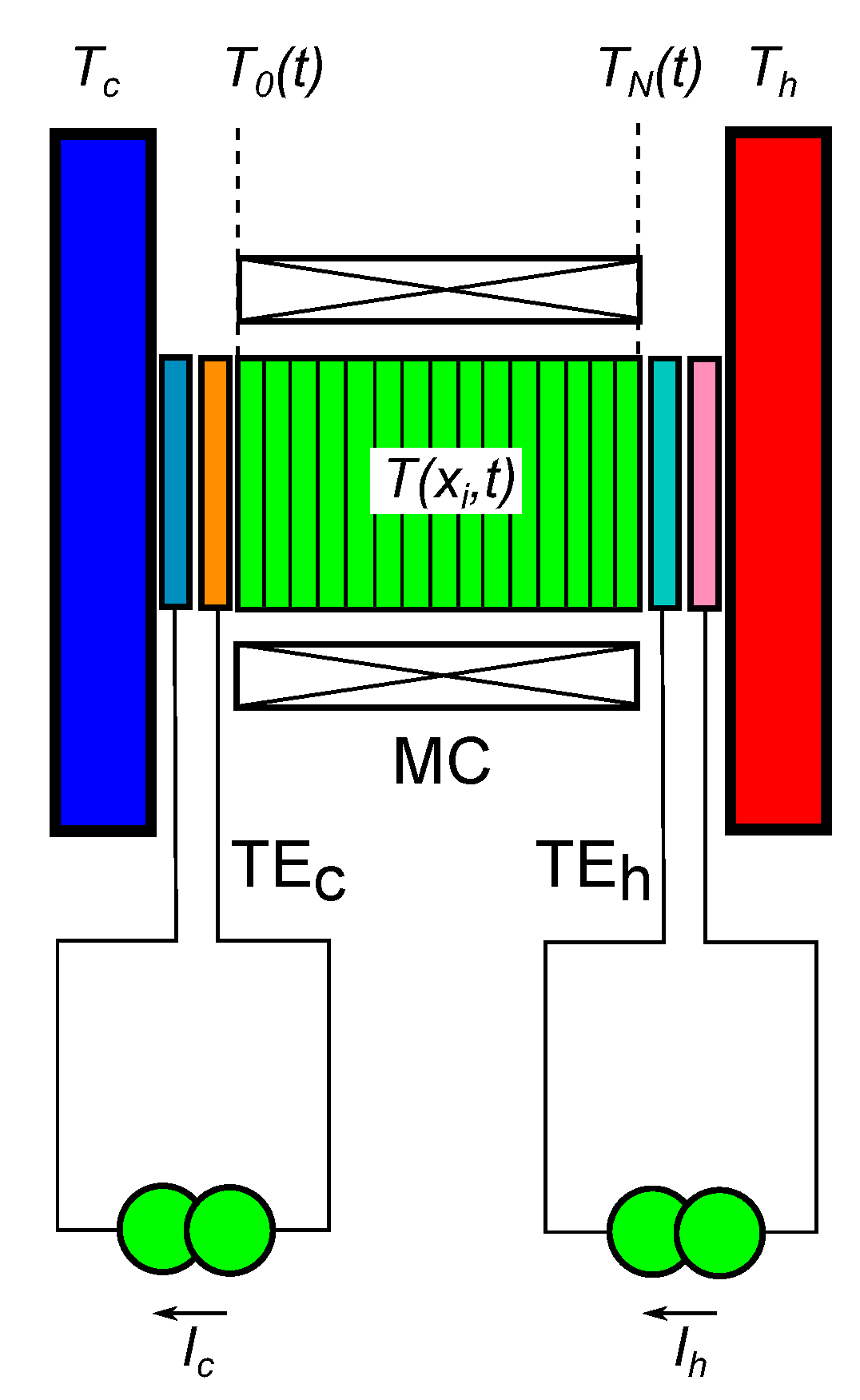This occurs because the TE method has low efficiency for a high temperature span $\mathrm{\Delta }T=T_h-T_c$, but increases strongly for low, or even negative, $\mathrm{\Delta }T$, which can be supplied by the MC subsystem. As outlined in Figure 1, a TE-MC-TE sandwich is placed between a cold heat source at temperature $T_c$ and a hot heat sink at $T_h$. An alternating magnetic field is applied to the MCM. When the magnetic field is on, the MCM is at its highest temperature, close to $T_h$. Then, the right-side TE cell is activated and pumps heat from the MCM to the hot sink. When the magnetic field is off, the MCM is cold, eventually being near or colder than $T_c$. The left side TE cell is then activated, transferring heat from the cold source to the MCM. De Vries and van der Meer [10] performed a simulation of a similar system, concluding that the cooling capacity was similar to that of Peltier cells alone, but their system used a fluid as a regenerator. Moreover, it is likely that the working parameters were not optimized. Huang et al. [11], very recently, reported a simulation for a complete MC system using Peltier cells as thermal diodes. This study involved simulation of Gd as the MC material and obtained moderate efficiencies. The key problem, that of using a material with second-order transition, was diluted among many other influences on heat losses and leaks. We presented some preliminary results of the simulation of a single sandwich in the conference THERMAG VIII [12], concluding that the TE-MC hybrid system was an interesting procedure, but that there were many variables to be optimized. Monfared [13] simulated a battery of sandwiches which were designed to reach higher temperature spans.

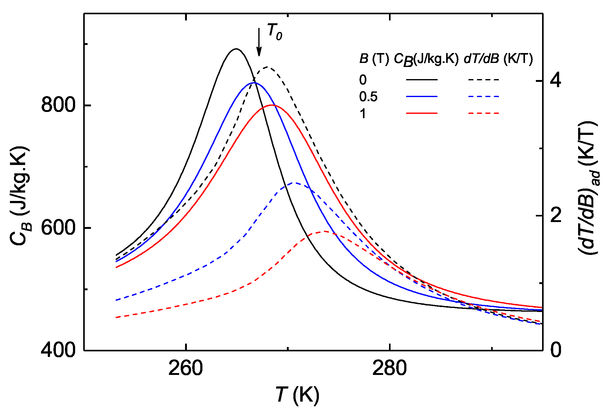
In this investigation, we found that the properties and dimensions of the MCM require to be correlated with the TE cells to achieve optimum performance in $COP$ or in cooling power. We simplified the properties of a TE cell, characterizing it with only three parameters: the effective Seebeck coefficient $ϵ$, the electrical resistance $R_0$, and the thermal conductance $\mathrm{\Lambda }$. The simulations undertaken take into account the properties of commercial TE cells. For the MCM, a material with a first-order transition and low hysteresis provides virtually infinite heat capacity, which is crucial to improve the efficiency. This is because, in the coexistence paramagnetic/ferromagnetic phase, the temperature is entirely determined by the magnetic field. The experimental properties of some doped La(Fe,Si)${}_{13}$ alloys are considered. A new master equation is derived for the heat transfer in the MCM, since the most used equation [13] is not valid for a material with a first-order transition, leading to a $\infty /\infty$ indetermination. The output of the simulation program ($COP$, magnetocaloric and thermoelectric work, extracted and released heat, etc.) is monitored for very slow continuous variation of certain working parameters. To simplify the case, only one sandwich is focused on, considering that a battery is essentially a superposition of sandwiches.

The potential applications of the system are not different to those of a refrigeration system with MC or TE materials, and are not discussed further here. The object of this investigation is to show that the combined TE-MC system results in higher efficiency and versatility than that achieved for pure magnetocaloric or thermoelectric systems.

Section 2 describes a simplified, but very faithful, model of the operation of a typical commercial Peltier cell. Section 3 presents, in a simplified manner, the working principles of a hybrid TE-MC system using materials with a first-order transition, such as La(Fe,Si)${}_{13}$, to highlight the essential details. Section 4 describes a numerical simulation using realistic parameters. Section 4.1 introduces an original master equation for the heat flow in an MCM having a first-order transition and the finite difference approximation that is used to solve the master equation. Section 4.2 discusses the realistic values for the working parameters. The following sub-sections present the simulation results for the cooling efficiency, the extracted and released heat powers, and the thermal evolution for the three cases being compared. A pure Peltier system is described in Section 4.3, a pure MC system with quasi-ideal thermal diodes is described in Section 4.4, and the combined MC-TE system with two Peltier cells and one MCM is described in Section 4.5. Finally, Section 5 presents the conclusions from a comparison of the three systems.

2. Model for Thermoelectric Cells

The effective values of $ϵ$, $R_0$, and $\mathrm{\Lambda }$ for a module consisting of many thermoelectric elements were used. The modelization was tested using the reported curves of extracted heat power ${\dot{Q}}_c$ against the temperature difference $\mathrm{\Delta }T$ for several electric current supplies I, and against the voltage V for different I values. In particular, the data for a cell from RTM Ltd. were tested against the model.

From first principles of irreversible thermodynamics [14], assuming a constant Seebeck coefficient, the voltage in a Peltier cell connected between two heat sources/sinks at temperatures $T_1$ and $T_2$ is,

$$V=ϵ(T_2-T_1)+R_{0}I$$

(2)

The extracted heat power from side 1 (let us assume the cold side), ${\dot{Q}}_1$, the heat power released to side 2 (the hot side), ${\dot{Q}}_2$, and the work power supplied by the cell, $\dot{W}$, are given by

$${\dot{Q}}_1=T_1ϵI+\mathrm{\Lambda }(T_1-T_2)-\frac{1}{2}{R}_0{I}^2$$

(3)

$${\dot{Q}}_2=T_2ϵI+\mathrm{\Lambda }(T_1-T_2)+\frac{1}{2}{R}_0{I}^2$$

(4)

$$\dot{W}={\dot{Q}}_2-{\dot{Q}}_1=(T_2-T_1)ϵI+R_0{I}^2=VI$$

(5)

From these equations, it follows that if $R_0\to 0$ and $\mathrm{\Lambda }\to 0$, $COP={\dot{Q}}_1/\dot{W}\to T_1/(T_2-T_1)$, and then, the efficiency of a Peltier cell is the Carnot efficiency. A very important detail is that, for small temperature differences, the conduction term can be neglected, resulting in

$$COP(\mathrm{\Delta }T\to 0)\simeq \frac{T_1-0.5R_{0}I/ϵ}{T_2-T_1+R_{0}I/ϵ}$$

(6)

For the cell 1ML07-050-15AN25 from RMS Ltd. at $T_2=298$ K, the parameters set are (

Table 1. Typical parameters used in the calculation for a TE-MC sandwich with an ideal MCM working in the phase coexistence region. The TE cells used are model 1ML07-050-15AN25 from RMT Ltd.

Symbol	Value	Units	Description
$2\tau$	2	s	Period
$T_c,T_h$	273, 275	K	Cold source and hot sink temperatures
$\mathrm{\Delta }T$	$T_h-T_c$	K	Temperature difference
TE cells
$ϵ$	25	mV/K	Effective Seebeck coefficient
$\mathrm{\Lambda }$	55	mW/K	Thermal conductance
$R_0$	1.0	$\mathrm{\Omega }$	Electric resistance
$I,I_c,I_h$	0.04–1.0	A	Currents in the TE cells
V		V	Voltage in a TE cell
$I_{1c},I_{2c}$	0.04–1.0	A	Max. and min. currents in the cold TE cell
$I_{1h},I_{2h}$	0.04–1.0	A	Min. and max. currents in the hot TE cell
MC material
$T_m,T_M$	267–281	K	Min. and max. MCM temperature
B	0–1.5	T	Magnetic field
$B_0$	1.5	T	Maximum magnetic field
$T_0$	267–273	K	Transition temperature at 0 T
$\beta =dT/dB$	4	K/T	Slope of the phase coexistence line
$\alpha$	1		Efficiency coefficient of the MC subsystem
Results
${\dot{Q}}_{1c},{\dot{Q}}_{2c}$		W	Heat power extracted at $T_m,T_M$
${\dot{Q}}_{1h},{\dot{Q}}_{2h}$		W	Heat power released at $T_m,T_M$
${\dot{Q}}_{1i},{\dot{Q}}_{2i}$		W	Heat power supplied to the MCM at $T_m,T_M$
${\dot{Q}}_{1f},{\dot{Q}}_{2f}$		W	Heat power extracted from MCM at $T_m,T_M$
$Q_c,Q_h$		J	Integrated extracted and released heats
$W_c,W_h$		J	Work performed by the cold and hot TE cells
$W_M$		J	Magnetic work
W		J	Total work
$COP$	$Q_c/W$		Coefficient of performance

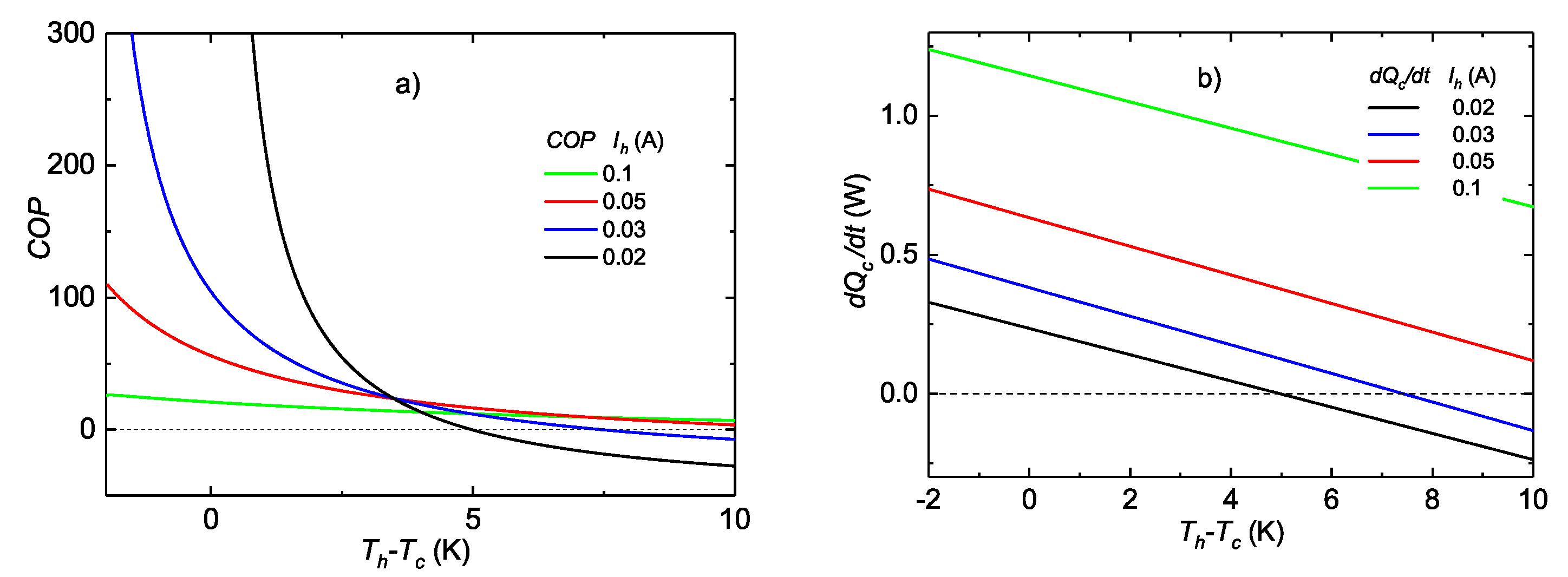
) $R_0=1.0$$\mathrm{\Omega }$, $\mathrm{\Lambda }=55$ mW/K and $ϵ=25$ mV/K (the cell is a combination of many TE elemental couples). For $T_2-T_1=0$, $COP=4.47/I\left(\mathrm{A}\right)-1/2$, producing an enormous value for low currents. For instance, for $I=0.1$ A, $COP=44.2$. For a negative temperature difference $T_2-T_1=-1$ K, and $I=0.1$ A, $COP=52$. However, for higher positive differences, the performance decays rapidly and the cell can barely transfer heat to the hot side if $T_2-T_1\ge 7.823$ K ($\dot{Q_1}\le 0$) with $I=$ 0.1 A. Nevertheless, it is able to prevent heat leakage from the hot side to the cold side.

A magnetocaloric material (i.e., a LaFeSi-type alloy) can increase the temperature by $\mathrm{\Delta }{T}_{MC}\simeq 4$ K upon application of a magnetic field, making the transfer possible very efficiently, for starting $T_2-T_1<\mathrm{\Delta }{T}_{MC}$. Consequently, the statement in [10] that the hybrid system produces the same performance as a TE system, is only valid for a particular, and not very fortunate, choice of parameters, but it is not generalizable. It is most likely that, in the simulation performed in this study, the Peltier subsystem was much more powerful than the MC system, preventing its effective action. Both subsystems should be adequately dimensioned.

3. Simple Model for a Sandwich Having an Ideal MCM with a First-Order Transition

The typical values of the parameters used in this section are listed in Table 1.

In this section, to establish the main physical principles of the combined system, we perform some simple mathematics using a proposed model for a TE cell and a simple model for the behavior of the MCM in the phase coexistence region. Let us assume that there is a heat “reservoir” (it will be seen that this has to be a heat pump), representing the MCM, that is assumed to be of infinite heat capacity at temperature T, regulated externally by a magnetic field. An MCM with a first-order transition fulfills these conditions under paramagnetic/ferromagnetic phase coexistence. As a simple case, let us consider that T has a constant low value, $T_m$, for a time $\tau$ and a higher value, $T_M$, for the same time, the period being $2\tau$. Let us assume that we apply some electrical current to the high and low temperature cells $I_h$ and $I_c$ in the following way

$$\begin{array}{c}\hfill 0<t<\tau :T=T_m;I_h=I_{1h},I_c=I_{1c}\end{array}$$

(7)

$$\begin{array}{c}\hfill \tau <t<2\tau :T=T_M,I_h=I_{2h},I_c=I_{2c}\end{array}$$

(8)

with constant values of $I_{1c}$, $I_{2c}$, $I_{1h}$ and $I_{2h}$. The current $I_{2c}$ is intended to prevent heat leakage to the cold source at $T_c$, through the TE cell on the left side (the cold TE cell), when the MCM is at its highest temperature $T_M$. During this time, the cold TE cell plays the role of a thermal diode, but it requires a small electrical work supply to achieve this purpose. $I_{1c}$ is intense enough to extract heat from the cold source when the MCM is at its lower temperature, $T_m$, and the transfer can be performed efficiently. During this stage, the TE cell is an active device. Similarly, in the hot TE cell, $I_{1h}$ prevents heat leakage to the MCM, when it is at $T_m$, and $I_{2h}$ transfers heat from the MCM when it is at $T_M$ to the hot sink at $T_h$. We also assume that the change between $T_m$ and $T_M$ takes a negligible time. In the interim, the magnetic subsystem performs an adiabatic process from $T_m$ to $T_M$ or vice versa. This assumption is an idealization, but not far removed from the real case. Equations (3)–(5), replacing $T_1$ and $T_2$ by the temperatures at both sides of each cell, give the following instantaneous heat powers extracted from the cold source by the cold TE cell: ${\dot{Q}}_c$, released to the intermediate system, ${\dot{Q}}_i$, extracted from the intermediate system by the hot TE cell, ${\dot{Q}}_f$, released to the hot source, ${\dot{Q}}_h$, and the work power made by each cell, ${\dot{W}}_c$ and ${\dot{W}}_h$. We assign the subscript 1 or 2 to these powers, according to the temperature of the intermediate MCM, obtaining

$$\begin{array}{c}\hfill 0<t<\tau (T=T_m):\end{array}$$

$$\begin{array}{c}\hfill {\dot{Q}}_{1c}=T_cϵI_{1c}+\mathrm{\Lambda }(T_c-T_m)-\frac{1}{2}{R}_0{I}_{1c}^2;{\dot{Q}}_{1h}=T_hϵI_{1h}+\mathrm{\Lambda }(T_m-T_h)+\frac{1}{2}{R}_0{I}_{1h}^2\end{array}$$

(9)

$$\begin{array}{c}\hfill {\dot{Q}}_{1i}=T_mϵI_{1c}+\mathrm{\Lambda }(T_c-T_m)+\frac{1}{2}{R}_0{I}_{1c}^2;{\dot{Q}}_{1f}=T_mϵI_{1h}+\mathrm{\Lambda }(T_m-T_h)-\frac{1}{2}{R}_0{I}_{1h}^2\end{array}$$

(10)

$$\begin{array}{c}\hfill {\dot{W}}_{1c}=(T_m-T_c)ϵI_{1c}+R_0{I}_{1c}^2;{\dot{W}}_{1h}=(T_h-T_m)ϵI_{1h}+R_0{I}_{1h}^2\\ \hfill \tau <t<2\tau (T=T_M):\end{array}$$

(11)

$$\begin{array}{c}\hfill {\dot{Q}}_{2c}=T_cϵI_{2c}+\mathrm{\Lambda }(T_c-T_M)-\frac{1}{2}{R}_0{I}_{2c}^2;{\dot{Q}}_{2h}=T_hϵI_{2h}+\mathrm{\Lambda }(T_M-T_h)+\frac{1}{2}{R}_0{I}_{2h}^2\end{array}$$

(12)

$$\begin{array}{c}\hfill {\dot{Q}}_{2i}=T_MϵI_{2c}+\mathrm{\Lambda }(T_c-T_M)+\frac{1}{2}{R}_0{I}_{2c}^2;{\dot{Q}}_{2f}=T_MϵI_{2h}+\mathrm{\Lambda }(T_M-T_h)-\frac{1}{2}{R}_0{I}_{2h}^2\end{array}$$

(13)

$$\begin{array}{c}\hfill {\dot{W}}_{2c}=(T_M-T_c)ϵI_{2c}+R_0{I}_{2c}^2;{\dot{W}}_{2h}=(T_h-T_M)ϵI_{2h}+R_0{I}_{2h}^2\end{array}$$

(14)

These equations are trivially integrated to give the extracted and released heats by every subsystem and the thermoelectric work in a cycle resulting

$$\begin{array}{c}\hfill Q_c=\tau \left[ϵT_c(I_{1c}+I_{2c})+\mathrm{\Lambda }(2T_c-T_m-T_M)-\frac{1}{2}{R}_0(I_{1c}^2+I_{2c}^2)\right]\end{array}$$

(15)

$$\begin{array}{c}\hfill Q_h=\tau \left[ϵT_h(I_{1h}+I_{2h})+\mathrm{\Lambda }(T_m+T_M-2T_h)+\frac{1}{2}{R}_0(I_{1h}^2+I_{2h}^2)\right]\end{array}$$

(16)

$$\begin{array}{c}\hfill Q_i=\tau \left[T_mϵI_{2c}+T_MϵI_{1c}+\mathrm{\Lambda }(2T_c-T_m-T_M)+\frac{1}{2}{R}_0(I_{1c}^2+I_{2c}^2)\right]\end{array}$$

(17)

$$\begin{array}{c}\hfill Q_f=\tau \left[T_mϵI_{1h}+T_MϵI_{2h}+\mathrm{\Lambda }(T_m+T_M-2T_h)-\frac{1}{2}{R}_0(I_{1h}^2+I_{2h}^2)\right]\end{array}$$

(18)

$$\begin{array}{c}\hfill W_c=\tau \left[(T_m-T_c)ϵI_{1c}+(T_M-T_c)ϵI_{2c}+R_0(I_{1c}^2+I_{2c}^2)\right]\end{array}$$

(19)

$$\begin{array}{c}\hfill W_h=\tau \left[(T_h-T_m)ϵI_{1h}+(T_h-T_M)ϵI_{2h}+R_0(I_{1h}^2+I_{2h}^2)\right]\end{array}$$

(20)

The intermediate “reservoir” should actually be a thermodynamic heat pump which receives ${\dot{Q}}_i$ at a temperature $T_m$ or $T_M$ and transfers ${\dot{Q}}_f$, making a work value of $W_M$ in a cycle. We assume that the intermediate system works cyclically, without any thermal connection with the environment (in a real device this point is not fulfilled, since the magnetic subsystem has a weak thermal leakage to or from the environment). Hence, the work performed by the magnetic subsystem is $W_M=Q_f-Q_i$ and the total work $W=W_c+W_h+W_M=Q_h-Q_c$. For compatibility with the second law of thermodynamics, the entropy released by the intermediate device should be higher than that extracted; this is

$$\begin{array}{c}\hfill \tau \alpha \left(\frac{{\dot{Q}}_{1i}}{T_m}+\frac{{\dot{Q}}_{2i}}{T_M}\right)=\tau \left(\frac{{\dot{Q}}_{1f}}{T_m}+\frac{{\dot{Q}}_{2f}}{T_M}\right)\end{array}$$

(21)

with $\alpha \ge 1$. The value $\alpha =1$ holds for an ideal Carnot device, working without entropy production.

Moreover, the value of $W_M$ is determined by the properties of the MCM for a given $T_m$ and $T_M$ (i.e., $W_M$ is the area of the thermodynamic cycle in the magnetization/field or entropy/temperature diagrams for that substance), which imposes another relation between $Q_i$ and $Q_f$. The pair of relations (17) and (18), involving $T_m$, $T_M$, $I_{1c}$, $I_{2c}$, $I_{1h}$, and $I_{2h}$, indicate that only four of these six quantities can be chosen arbitrarily. Let us assume that $\alpha =1$ and the four currents through the TE cells are fixed. Then, the intermediate system has to adapt its maximum and minimum temperatures $T_m$ and $T_M$ to achieve the Carnot efficiency, since the extracted and released heats are determined by the currents at the TE cells. If the MCM is a typical ferromagnet without a phase transition (strictly, a second-order transition at the Curie temperature occurs only at zero field, but there is no transition for any other field in a typical ferromagnet), the steady regime is reached when Equation (21) is obeyed and $W_M=Q_f-Q_i$.

In an MCM with a first–order transition, such as a La(Fe,Si)${}_{13}$ alloy, working in the phase coexistence region, the temperatures $T_m$ and $T_M$ are both determined by the minimum and maximum magnetic fields (this is a requirement of the Gibbs phase rule, i.e., the state of the MCM is a point of the phase coexistence line in a $B/T$ diagram and B determines the temperature). However, if the relation (21) is not fulfilled, the MCM will gain or lose net heat every cycle (then, $W_M\ne Q_f-Q_i$). This net heat will gradually transform one phase to the other phase and the material will change to a single-phase state when one of the phases is exhausted. After this, the temperature of the resulting phase, $T_m$ or $T_M$, will change slowly until Equation (21) is satisfied, reaching a steady regime. It is desirable to have the MCM in the phase coexistence region as long as possible, where the MC effect is much more powerful. Most often, the lowest magnetic field is zero, and then $T_m$ is the transition temperature at zero field, $T_0$, (frequently referred to as the Curie temperature, but its character differs markedly from that of a typical ferromagnet). On the other hand, the phase coexistence line is very approximately a straight line $T=T_0+\beta B$ and $T_M$ is determined by the maximum applied field. Therefore, for an MCM with a first-order transition, and for a maximum applied field B, only three parameters can be chosen among $I_{1c}$, $I_{2c}$, $I_{1h}$, and $I_{2h}$, if we want to work in the steady regime and always in the phase coexistence region. For instance, if we apply equal currents to both TE cells, making $I_{1c}=I_{2h}$ and $I_{2c}=I_{1h}$ (two constraints), the MCM will leave the coexistence state region before reaching the steady regime, except for the precise value of the magnetic field B, which determines $T_M$, such that the relation (21) is satisfied.

A natural working hypothesis is to take $I_{2c}$ and $I_{1h}$ as the minimum values which prevent thermal leakage from the MCM to the cold source and from the hot sink to the MCM. This is achieved in Equation (12) imposing ${\dot{Q}}_{2c}=0$ and in Equation (10) ${\dot{Q}}_{1f}=0$. These relations determine the two low currents. We can arbitrarily choose the maximum current at the cold cell, $I_{1c}$, which determines the heat-per-cycle extracted from the cold source, according to Equation (15). With given $T_m$ and $T_M$, and chosen $I_{1c}$, $I_{2c}$, and $I_{1h}$, Equation (21) gives the value of $I_{2h}$ for the steady regime. The cooling power, $Q_c/2\tau$, and the other heat and work values are obtained via Equations (15)–(20). Finally the COP in the steady regime is computed as

$$COP=\frac{Q_c}{W}=\frac{Q_c}{Q_h-Q_c}$$

(22)

Assuming the linear dependence of T with B for the phase coexistence line, $T_0$ can be tailored by manipulating the chemical composition of several MC alloys. $\beta \simeq 4$ K/T for typical alloys derived from La(Fe,Si)${}_{13}$. Let us assume that the magnetic subsystem follows a Carnot cycle between the magnetic fields 0 and B. Then, the temperatures of the MCM are $T_m=T_0$ and $T_M=T_0+\beta B$. The steady regime, while keeping the MCM in the phase coexistence region, imposes the relation of Equation (21).

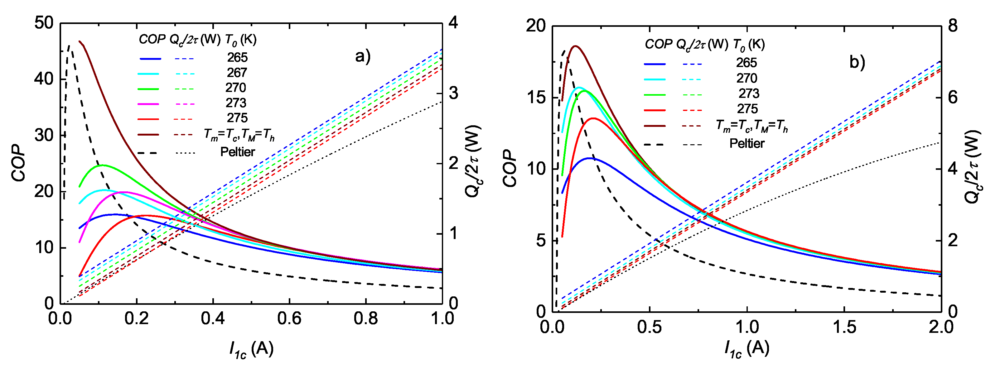
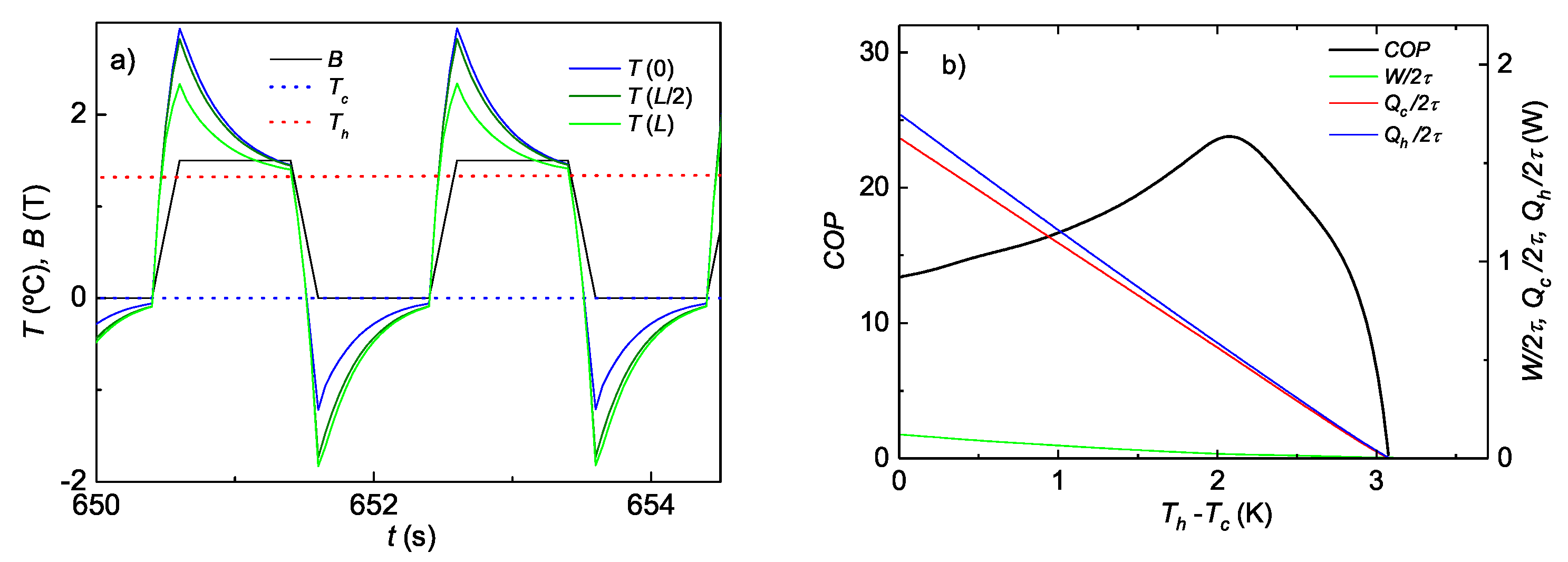
Figure 2a shows $COP$ and the cooling power $Q_c/2\tau$ for $T_c=273$ K, $T_h=275$ K ($\mathrm{\Delta }T=$ 2 K), for several characteristic temperatures of the MCM and a fixed increment $T_M-T_m=\beta B=8$ K. For the interesting case, included in the figures, in which the low and high temperatures of the MCM coincide with the temperatures of the cold source and the hot sink, respectively, $T_m=T_c$ and $T_M=T_h$, the magnetic field is adjusted to be $B=(T_h-T_c)/\beta$ instead of 2 T. This figure also shows the data for a pure Peltier heat transfer; that is, two Peltier cells in series, working continuously, with the same current, $I_{1c}$, without any intermediate system. To compare with the hybrid system, the power of the pure Peltier method is divided by two, because, in the hybrid system, each cell works actively only during one half of the period.

The curves in Figure 2a show how the choice of the transition temperature of the material, $T_0$ at zero field, and the applied magnetic field, which fixes the maximum temperature of the MCM, are critical. For a cold source at $T_c=273$ K and a hot sink at $T_h=275$ K, and a maximum applied field of 2 T (therefore, $T_M=281$ K), the maximum COP is obtained for $T_0=270$ K, and decays sharply for higher or lower values. If $T_0=T_m=T_c$ and the magnetic field is regulated to reach the maximum temperature $T_M=T_h$, the efficiency (brown curve in Figure 2a) increases dramatically and overcomes that of a pure Peltier system by a large amount, doubling its COP except for very low heat flow given for low currents. Similar features occur, but with lower COP, for a higher temperature span. 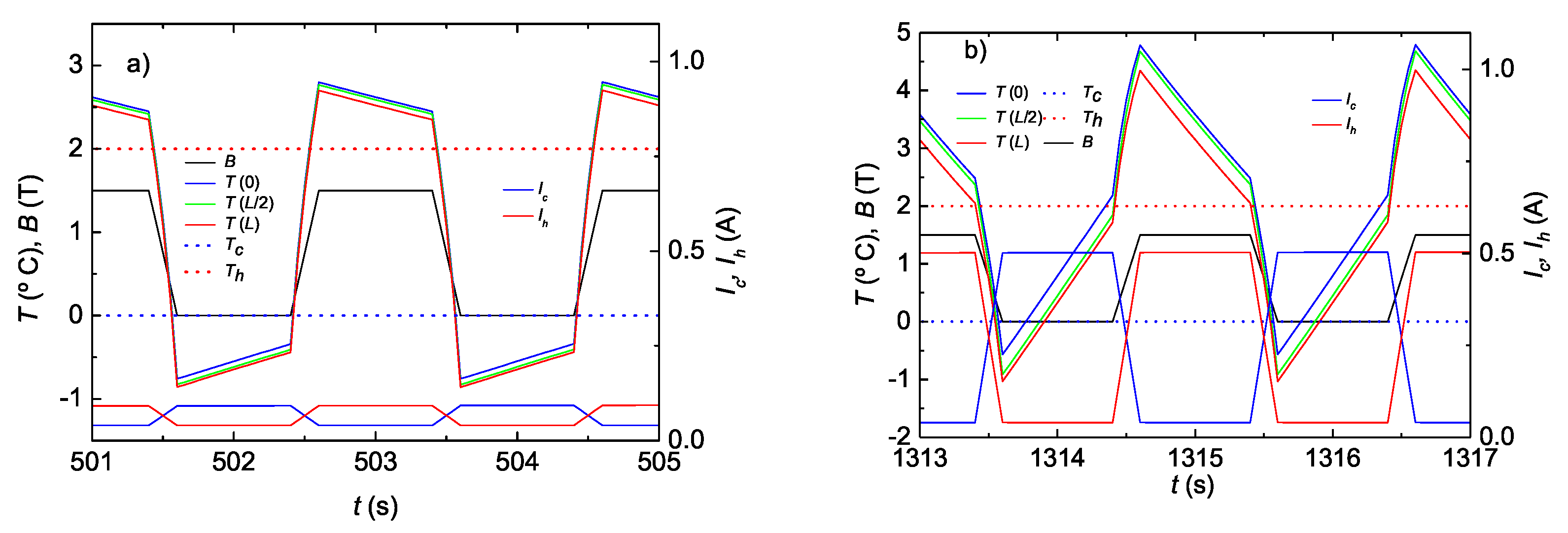Figure 2b shows the results for $T_c=273$ K and $T_h=278$ K. Except for very weak currents, the $COP$ is clearly higher for the hybrid system, even more than twice in most of the range $I_{2c}=I_{1c}<1$ A. The cooling power is also greater than that of the pure Peltier method. The $COP$ of the hybrid system decreases if $T_m>T_c$ (e.g., for $T_m=T_0=275$ K) or $T_M<T_h$ (e.g., for $T_m=T_0=265$ K, $T_M=T_0+8$ K = 273 K). The highest $COP$ occurs if the MCM and the magnetic field are chosen to have $T_m=T_c$ and $T_M=T_h$ (brown curves in Figure 2).

As the main conclusion of this section, a hybrid sandwich in which the MCM has a first-order transition improves the efficiency with respect to a pure TE system if working in the phase coexistence region, but the working parameters have to be properly chosen.

4. Numerical Simulation

The ideal case described in Section 3 shows a significant advantage of the hybrid system against the pure Peltier system with the same cells, but the behavior of a real MCM is neither so simple, nor so efficient. In this section, we describe a numerical simulation for a more realistic case, taking the measured properties of a La(Fe,Mn,Si)${}_{13}$H${}_{1.65}$ alloy, including real dimensions. A 1D simulation for the spatial distribution requires little computation time and allows for many different conditions to be tested.

4.1. Master Equation

For the heat transfer in the MCM, the following equation is used

$$\frac{\partial T}{\partial t}=\frac{1}{\rho C_B}\overrightarrow{\nabla }·\left(\lambda \overrightarrow{\nabla }T\right)+{\left(\frac{\partial T}{\partial B}\right)}_{ad}\frac{dB}{dt}$$

(23)

where $\rho$ is the density, $C_B$ is the field-dependent specific heat, and $\lambda$ is the thermal conductivity of the MCM. This equation is slightly different than the widely used Equation (2) of [13], where the adiabatic temperature change with the field, ${\left(\partial T/\partial B\right)}_{ad}$, is replaced by $(-T/C_B){\left(\partial S/\partial B\right)}_T$. Actually, both expressions are equivalent in equilibrium thermodynamics, but not necessarily in the case of a material with a hysteretic first-order transition. Moreover, in Equation (2) of [13], both factors ${\left(\partial S/\partial B\right)}_T$ and $C_B$ depend strongly on the field and temperature. Therefore, their ratio is ill-conditioned and experimental errors in the parameters can lead not only to wrong results, but also to results incompatible with the fundamental laws of thermodynamics, for instance, if the heat capacity is taken for granted as a constant. The above master equation solves this problem for the actual numerical simulation. In a first-order transition, $(T/C_B){\left(\partial S/\partial B\right)}_T$ involves a $\infty /\infty$ indetermination, when both $C_B\to \infty$ and ${\left(\partial S/\partial B\right)}_T\to \infty$. Using experimental data, these quantities are not infinite, but produce an ill-conditioned value (i.e., in the phase coexistence region $C_B$ can change enormously with slight temperature or field changes, or from one sample to another of the same compound, or even in different thermal cycles of the same material). On the other hand, in a first-order transition, ${\left(\partial T/\partial B\right)}_{ad}$ is the slope of the transition line in a $T/B$ diagram and is very well-determined. Incidentally, ${\left(\partial T/\partial B\right)}_{ad}$ can be constant only if it is zero or if $C_B\to \infty$, as happens in a first-order transition while two phases coexist.

A 1D Crank–Nicolson (CN) [15] finite difference approximation was used for Equation (23). The position $0\le x\le L$ of $N+1$ discrete points of the MCM is considered at $x_i=i\mathrm{\Delta }x,i=0,1,\dots ,N$, with $\mathrm{\Delta }x=L/N$, at the time values $t_n=n\mathrm{\Delta }t,n=0,1,2,\dots$. Assuming constant $\lambda$, the master equation is replaced by the approximate system

$$\begin{array}{c}\hfill T_i^{n+1}=T_i^n+\frac{1}{2}{D}_i^n(T_{i-1}^n+T_{i+1}^n-2T_i^n)+\frac{1}{2}{D}_i^{n+1}(T_{i-1}^{n+1}+T_{i+1}^{n+1}-2T_i^{n+1})+\\ \hfill +\frac{1}{2}{\tau }_i^n\frac{dB\left(t_n\right)}{dt}+\frac{1}{2}{\tau }_i^{n+1}\frac{dB\left(t_{n+1}\right)}{dt}\end{array}$$

(24)

being $T_i^n=T(x_i,t_n)$, $D_i^n=\lambda \mathrm{\Delta }t/\left[\rho C_B(T_i^n,B\left(t_n\right))\mathrm{\Delta }{x}^2\right]$, ${\tau }_i^n=\mathrm{\Delta }t{\left(\partial T_i^n/\partial B\right)}_{ad}$. The error of this approximation is of the order of $\mathrm{\Delta }{t}^2$ for the time derivative and of $\mathrm{\Delta }{x}^2$ for the second derivative with respect to x. This is one order of approximation better than for the explicit or implicit Euler methods. Moreover, the CN method always converges and there is no restriction to the values of the parameters $D_i^n$ and ${\tau }_i^n$, putting aside restrictions related to the precision desired in the calculation.

The boundary conditions are imposed by the energy conservation at the edges of the MCM, according to the heat flux between the MCM and the TE cells

$$\begin{array}{cc}\hfill x=0;& \frac{\lambda A}{\mathrm{\Delta }x}(T_0^n-T_1^n)=T_0^nϵI_c+\mathrm{\Lambda }(T_c-T_0^n)+\frac{1}{2}{R}_0{I}_c^2\\ \hfill x=L;& \frac{\lambda A}{\mathrm{\Delta }x}(T_{N-1}^n-T_N^n)=T_N^nϵI_h+\mathrm{\Lambda }(T_N^n-T_h)-\frac{1}{2}{R}_0{I}_h^2\end{array}$$

(25)

with A being the section of the MCM, and $I_c$, $I_h$, the currents trough the TE cells at the cold and hot sides.

The set of Equations (24) and (25) form a non-linear system, since $D_i^n$ and ${\tau }_i^n$ depend on the instantaneous temperature and magnetic field at every point. Knowing the temperatures $T_i^n$ at any time $t_n$, the solution of the system gives the values at the next time step, $t_{n+1}$. The solution can be obtained by the iterative Gauss–Seidel method. The first iteration starts by taking $T_i^{n+1}=T_i^n$, $D_i^{n+1}=D_i^n$, and ${\tau }_i^{n+1}={\tau }_i^n$ at the right side of Equation (24) and obtaining explicitly a new set of values for the time $t_{n+1}$. The calculation is repeated, inserting the new values in the right side, until a desired convergence is reached. The whole procedure was achieved with a home-made FORTRAN code.

4.2. Typical Parameters

The set of parameters used for each simulation is specified in the corresponding subsection.

Table 2. Typical parameters used in the numerical simulation. The parameters which cover a range of values, except $t_{end}$, can vary slowly and linearly with time from $t_{start}$ to $t_{end}$.

Symbol	Value	Units	Description
MC material:	La(Fe,Mn,Si)${}_{13}$H${}_{1.65}$
$T_0$	267	K	Transition temperature at 0 T
$\lambda$	100	W/m·K	Thermal conductivity
$C_B$	function	J/kg·K	Heat capacity
${(\partial T/\partial B)}_{ad}$	function	K/T	MCE
$\rho$	7260	kg/m${}^3$	Density
L	2.5	mm	Length
A	1.0	cm${}^2$	Section
B	variable	T	Magnetic field
$B_0$	1.5	T	Maximum magnetic field
$T_c$	273.15	K	Cold source temperature
$T_h$	273.15–281.15	K	Hot sink temperature
$\mathrm{\Delta }T$	$T_h-T_c$	K	Temperature difference
Simulation
$2\tau$	2	s	Period
$\mathrm{\Delta }t$	$1.0\times {10}^{-4}$	s	Time step
$t_n=n\mathrm{\Delta }t$	variable	s	Simulated time
$t_{start}$	400	s	Time for steady regime
$t_{end}$	2000–5000	s	End of simulation
$x_i=iL/N$	variable	mm	Position in the MCM
N	16		Number of x intervals
$\mathrm{\Delta }x=L/N$	0.15625	mm	Step length
$D_i^n$	variable		Reduced diffusivity
${\tau }_i^n=\mathrm{\Delta }t{(\partial T_i^n/\partial B)}_{ad}$	variable	s·K/T	Reduced MCE

shows the typical values used when not explicitly specified. Most often, the simulation keeps all parameters constant for $t<t_{start}$ to reach a steady regime. After this time, one parameter varies slowly and linearly with time to produce a continuous plot of the results as functions of the variable parameter in a quasi-steady regime. There are slight differences with respect to the results for a true steady regime (which can be clearly observed upon passing from steady to quasi-steady), but this procedure saves computation time, avoiding waiting for the steady regime, for each value of the variable parameter.

The cold source is at a fixed temperature $T_c$, while the hot sink is at a variable or constant temperature, depending on the simulated case: $T_h=T_c+\mathrm{\Delta }T$ with $\mathrm{\Delta }T=0$–5 K (a small increment, considering the sandwich as a single element in a battery). The working parameters of the simulated Peltier cells are given in Table 1.

For the MCM, the experimental data tables for $C_B(T,B)$ and ${(\partial T/\partial B)}_{ad}$ of some La(Fe,Mn,Si)${}_{13}$H${}_{1.65}$ alloys have been taken as the basis for obtaining the simulated values. An interpolation procedure to obtain these properties for every value of T and B from the experimental data tables is not a trivial task (e.g., when $C_B\left(T\right)$ is a sharp function picked at the transition temperature for each measured field, for an intermediate field it is not the average, but a function picked at an intermediate temperature) as explained in [16]. Figure 3 shows the simulated values for $T_0=267.15$ K. A change in $T_0$ is simulated by a translation of $C_B$ and ${(\partial T/\partial B)}_{ad}$ along the T axis. The density $\rho =7260$ kg/m${}^3$ is taken as a typical value for these alloys. The thermal conductivity is enhanced to values about $\lambda =100$ W/(m·K), which can be obtained by intercalating copper sheets around the MCM. At a given field B, the coexistence temperature is not a single T value in a real material, due to inhomogeneities in composition, grain size, stress, etc. Considering the temperature for the $C_B$ maximum as the nominal phase coexistence $(T,B)$ point, the slope of the phase coexistence line is approximately $dT/dB\simeq 4$ K/T; this datum is implicitly included in the simulated function. Typical dimensions of the MCM are, section $A=1$ cm${}^2$, length $L=2.5$ mm. The temperature of the MCM is only saved and plotted at five representative points taken at $x=0,L/4,L/2,3L/4,L$. These are at the center, at the edges, and at half-way between the center and the edges.

The magnetic field B is varied in a quasi-square wave form (see Section 4.4 below) between 0 and $B_0\simeq 1.5$ T, with a typical frequency $\nu =0.5$ Hz, but simulations were also undertaken with other frequencies. In this wave shape, the field has a constant minimum value of zero and a constant maximum value for two-fifths of the period each, and it changes between these extremes, with ramps of one tenth of the period, seeking to emulate an ideal adiabatic magnetization or demagnetization, but with a realistic rate of change, for a rotating magnet [18]. The discretization parameters were taken to be smaller and smaller until no substantially different results were found. In the CN method, enhanced precision is achieved if $D_i^n<<1$.

From the $T_i^n$ values, the instantaneous heat and work powers are computed as ${\dot{Q}}_c$, ${\dot{Q}}_h$, and ${\dot{W}}_{TE}$ by Equations (3)–(5), applied to the cold and the hot Peltier cells, respectively. The heat power released by the MCM is ${\dot{Q}}_{MC}=\lambda A(T_1^n-T_0^n+T_{N-1}^n-T_N^n)/\mathrm{\Delta }x$. These powers are integrated over one cycle to obtain the integrated heat and work values $W=Q_h-Q_c$, assuming a quasi-steady regime, which is not true during the transient stage.

The magnetic work is $W_{MC}=Q_{MC}$ in a cycle. Finally, the performance coefficient is $COP=Q_c/(W_{TE}+W_{MC})=Q_c/(Q_h-Q_c)$.

4.3. Pure Thermoelectric Cooling

Figure 4a shows the temperature of the MCM at five points $x=0,L/4,L/2,$$3L/4,L$, with $t_{start}=100$ s and increasing the current supply $I_h=I_c$ through the TE cells, for $T_h-T_c=2$ K. The conductivity of the MCM was set to $\lambda =10$ W/m·K (ten times lower than in other simulations). At $t=118$ s, $I_h=0.008$ A, this weak current is enough to avoid heat leakage from the hot side to the cold side, since the T gradient is nearly zero in the MCM. For higher currents, the Peltier cells transfer heat from the cold side to the hot side. Figure 4b shows that $\dot{Q_c}$ increases with $I_h$, but reaches a maximum outside the figure. The maximum $CO{P}_{max}=44$, which is $32\%$ of $COP$(Carnot), occurs for $I_c=I_h=0.023$ A, a very high $COP$ value, but lower than that obtained for the same $\mathrm{\Delta }T$ without the MCM (see Figure 2a). This is due to the relatively low thermal conductivity of the MCM. The heat flow by conduction imposes a large T gradient, making the thermal jump greater than $(T_h-T_c)/2$ on each TE cell, which reduces its efficiency. Therefore, when the MCM does not play its role, it is a handicap for the system performance. A high conductivity of the MCM becomes critical. It can be increased by alternating copper sheets ($\lambda$(Cu) $\simeq 400$ W/m·K, forty times higher than that of the La(Fe,Si)${}_{13}$ alloys) parallel to the heat flow. For higher currents, $COP$ decreases rapidly as is usual in a TE refrigerator.

Figure 5a shows $COP$ of the pure TE system with an increasing temperature difference $\mathrm{\Delta }T=T_h-T_c$ for several current supplies, $I_h=I_c$, to both TE cells. For very weak currents, $COP$ reaches very high values for small or negative $\mathrm{\Delta }T$ (for negative $\mathrm{\Delta }T$, the Carnot $COP$ is also negative since the system transfers heat from $T_c$ (higher) to $T_h$ (lower) and produces work). For higher currents the system can pump heat across higher $\mathrm{\Delta }T$, but with low efficiency. Figure 5b shows the cooling power ${\dot{Q}}_c$, which decreases with $\mathrm{\Delta }T$ and increases with the current, for low currents. In particular, it is clear that, for $I_h=I_c=0.02$ A, the Peltier cells can transfer heat with high efficiency for $\mathrm{\Delta }T<2$ K and are able to stop heat leakage for $\mathrm{\Delta }T<5$ K. On the other hand, it is also clear that a Peltier system supplied with high current, $I_h=I_c>0.1$ A, does not benefit greatly from a small or negative $\mathrm{\Delta }T$. In our opinion, this is the cause of the small effect of the MCM in [10], where currents of 0.01 A might be too strong given the size of the Peltier cells used there.

4.4. Pure Magnetocaloric Cooling with Passive Thermal Diodes

Pure magnetocaloric cooling using thermal diodes can be simulated with the same program, fixing $I_h=I_c=0$, but imposing different conductances in opposite directions for the TE cells. Let ${\mathrm{\Lambda }}_r$ be the thermal conductance to the right side and ${\mathrm{\Lambda }}_l$ to the left side. We assume ${\mathrm{\Lambda }}_l=55$ mW/K to be equal to the real conductance of the Peltier cell 1ML07-050-15AN25 and ${\mathrm{\Lambda }}_r=100{\mathrm{\Lambda }}_l$. This high rectification ability is difficult to achieve with real thermal diodes [19], but serves to evaluate the pure MC refrigeration. Figure 6a shows the evolution of the temperatures at three points of the MCM described in Section 4.2, while the magnetic field varies as a quasi-square wave between 0 and $B_0=$ 1.5 T, with frequency $\nu =0.5$ Hz. The hot-side temperature $T_h$ is forced to increase linearly and slowly with time (this variation cannot be noticed in the time range plotted in Figure 6a), at $d{T}_h/dt=5.26$ mK/s, from $t_{start}$ = 400 s to the end of calculation, $t_{end}$ = 1219 s. The gradient of $T\left(x\right)$ is high during, and just after the end of, the field variation, but the MCM tends to thermal equilibrium with either the cold source or the hot sink during the time span of constant B. The frequency should be adjusted for the conductivity, dimensions, and properties of the material. The relaxation time of the MCM is ${\tau }_{relax}=\rho L^2{C}_B/\lambda \simeq 0.27$ s. This value should not be much lower than $1/\left(2\nu \right)$ (more precisely the time with constant field, which in the simulation of Figure 6a is $0.4/\nu =0.8$ s). If $\tau <<{\tau }_{relax}$, the system does not present any advantage and if $\tau >>{\tau }_{relax}$, the MCM reaches the thermal equilibrium with the hot or the cold source too early in each semi-period and spends a long time afterwards transferring no heat. Figure 6b shows $COP$ and the cooling power of the system with thermal diodes. The maximum $COP$ occurs for a given $\mathrm{\Delta }T$ value ($\simeq 2$ K in this example) which is determined by the material, the dimensions, and the magnetic field. All these parameters are difficult to change, assuming the magnetic field is produced by a permanent magnet. Therefore, the dimensions should be well-designed for a given application. The system with thermal diodes with La(Fe,Mn,Si)${}_{13}$H${}_{1.65}$ cannot pump heat for $\mathrm{\Delta }T>3$ K in a single stage with $B_0=1.5$ T, but the temperature jump can be increased using several sandwiches in series, with alternate fields on consecutive elements.

4.5. Hybrid MC-TE Cooling with La(Fe,Mn,Si)${}_{13}$H${}_{1.65}$

Figure 7 shows a few periods of the evolution of the temperatures at five points along the length of the MCM for a simulation where the currents at the TE cells, $I_c\left(t\right)$, $I_h\left(t\right)$, and the magnetic field $B\left(t\right)$ are varying as quasi-square waves. After reaching the steady regime, at $t_{start}$ = 400 s, the current amplitudes increase very slowly, starting at 0.04 A (estimated to prevent heat leakage) up to 1 A, always with constant magnetic field amplitude $B_0=1.5$ T and fixed temperatures of the cold source and the hot sink, $T_c=273$ K, $T_h=275$ K. The quasi-steady regime can always be assumed. The characteristic temperature (transition at zero field) of the MCM is $T_0=268.15$ K. Assuming a similar notation to that of Table 1 for the temperatures and currents ($T_m\left(t\right)$, $T_M\left(t\right)$, now time-dependent, are the average temperatures of the MCM when the field is off and on, respectively). As shown in Figure 7a, left panel (where the currents are low: $I_{1c}=I_{2h}\simeq 0.093$ A), when the field amplitude is increasing from 0 to $B_0$, the temperatures also increase, reaching a maximum, $T_{M,ini}>T_h$, at the time of maximum field. Then, the hot TE cell is activated, transferring heat to the hot sink. In contrast to an ideal system in phase coexistence, $T_M\left(t\right)$ depends on time (it also has a negative gradient allowing the heat to diffuse towards the right side edge). $T_M\left(t\right)$ decreases slowly and quasi-linearly (since the transferred heat power is approximately proportional to the current, constant in this stage), down to $T_{M,fin}$, at the end of the maximum field stage. Then, the hot TE cell is deactivated (i.e., with $I_h$ reduced to $I_{1h}=0.04$ A), and the field is rapidly decreased to zero in one tenth of the period. The temperatures drop down to a value $T_{m,fin}<T_c$. At this point the cold cell is activated and $T_m\left(t\right)$ increases slowly up to $T_{m,fin}$, while some heat is transferred from the cold source to the MCM. Finally, the cold TE is deactivated and the magnetic field is increased again, repeating the process quasi-periodically. The current amplitudes are very slowly increasing. This increase can barely be noticed within a few periods, but the different currents are clearly distinguished between $t\simeq 500$ s (Figure 7a) and $t\simeq 1300$ s (Figure 7b).

For the low currents shown in Figure 7a, $T_{M,fin}>T_h$ and $T_{m,fin}<T_c$. As sketched in Section 3, in the ideal working condition $T_m\simeq T_c$ and $T_M\simeq T_h$, which is not fulfilled by the simulated system for such low currents. Too wide a temperature oscillation interval of the MCM means a high $W_M$, which is not compensated for by the increase in the TE cells’ efficiency. For these low currents the frequency should be reduced. Figure 7b shows the same data for $I_{1c}=I_{2h}\simeq 0.50$ A. In this case, $T_m$ and $T_M$ decrease more markedly during the constant field time range. The interval is adequate for the value of $T_h-T_c$, but the averages are $\langle T_m\rangle >T_c$ and $\langle T_M\rangle >T_h$. As explained in Section 3, the MCM temperatures adapt themselves until the net heat flow per cycle to or from the MCM is zero. In this case, a material with a lower $T_0$ would be more appropriate.

Figure 8a shows the instantaneous heat powers extracted from the cold source and released to the hot sink. It can be observed that, when the magnetic field is high, the hot TE cell transfers heat to the hot sink and the cold TE cell extracts a small heat power from the cold source. However, when the field is zero, the cold TE cell extracts heat from the cold source and the lowest current is just enough to avoid heat leakage. Figure 8b shows the COP, the cooling and heating average powers, and the average work power per cycle, along those for a pure Peltier cooling. In the last case, the powers are divided by two, taking into account that, in the combined method, each cell is activated for one half of the period. Choosing suitable parameters, the COP and the cooling power are higher for the hybrid system, although lower than for an ideal Carnot device with the MC subsystem. In particular, for low currents, the COP can show a relevant increase. For instance, for $I_{c,max}=I_{h,max}=0.1$ A, $COP$ increases from 24 to 31. As a comparison, with these data, the pure MC cooling with ideal thermal diodes (Figure 6b) has a fixed cooling power $Q_c/2\tau =$ 0.56 W and $COP$ = 23.6, which can be compared with $COP=22.8$ obtained with the hybrid system for the same cooling power and the same $\mathrm{\Delta }T$.

5. Conclusions

A hybrid TE-MC-TE sandwich containing an MCM with a first-order transition was analyzed. A 1D finite difference simulation enabled testing of many working conditions without severe loss of relevance of the results. The virtue of the intermediate MC subsystem is the potential for increasing or decreasing its temperature under the action of a magnetic field B, enabling more efficient heat transfer of the adjoining TE cells. In comparison to a pure Peltier system, the calculation for an ideal MCM with a first-order transition, working in the phase coexistence region, has much higher efficiency, which highlights the possibilities of the combined method. When a more realistic system is simulated, using La(Fe,Mn,Si)${}_{13}$H${}_{1.65}$ as the MCM, $COP$ decreases significantly. However, with a good choice of working parameters, it is still higher than for a pure Peltier system with the same cells. The lower efficiency obtained for a real MCM is connected to the moderate thermal conductivity and the distribution of transition temperatures, which occurs in a real material, instead of having a sharp transition.

In comparison with pure MC cooling, using ideal thermal diodes, the hybrid system achieves almost the same efficiency, but with more versatility. The hybrid system can work with any cooling power (but with lower $COP$ for high powers), unlike the pure MC system, in which the cooling power is practically fixed. Finally, an open question is whether the much more complex set-up of the hybrid system compensates for the higher efficiency obtained.

This study can be extended in the future, to consider a complete cooling system with a hybrid TE-MC refrigerator, using the operating parameters selected based on the results of Section 3 and Section 4. Making random choices of the parameters would most likely lead to irrelevant results.