Low-Frequency Dynamic Magnetic Susceptibility of Antiferromagnetic Nanoparticles with Superparamagnetic Properties

Abstract

As is known, the multi-sublattice structure of antiferromagnets (AFMs) entails that, under size diminution to the nanoscale, compensation of the sublattice magnetizations becomes incomplete. Due to that, the nanoparticles acquire small, but finite permanent magnetic moments. An AC field applied to such particles induces their magnetic response, the measurement of which is well within the sensitivity range of the experimental technique. Given the small size of the particles, their magnetodynamics is strongly affected by thermal fluctuations, so that their response bears a considerable superparamagnetic contribution. This specific feature is well-known, but usually is accounted for at the estimation accuracy level. Herein, a kinetic model is proposed to account for the magnetic relaxation of AFM nanoparticles, i.e., the processes that take place in the frequency domain well below the magnetic resonance band. Assuming that the particles possess uniaxial magnetic anisotropy, the expressions for the principal components of the both linear static and dynamic susceptibilities are derived, yielding simple analytical expressions, including those for the case of a random distribution of the particle axes.

1. Introduction

In 1961, Louis Néel [1,2] predicted that nanoparticles of the materials that in the bulk phase are conventional antiferromagnets (AFM), i.e., the systems consisting of fully compensated spin sublattices, should possess, albeit weak, but quite discernible permanent magnetic moments. In other words, it had been established that there is no such object as a completely antiferromagnetic nanoparticle. Instead, one always deals with an entity whose magnetic response combines the contributions from: (i) its antiferromagnetic spin order, which ensures anisotropic susceptibility, and (ii) a permanent magnetic moment resulting from the decompensation of the sublattices, which otherwise have identical properties. This decompensation may have diverse origins, but the main two are: unequal spin populations of the sublattices due to the limited number N of atomic spins in the particle and an incomplete spin closely surrounding the particle surface. As surmised by Néel, the uncompensated magnetic moment ${\mu }_u$ should be of the order ${\mu }_{B}z{N}^{1/2}$ if the spin-site occupation fluctuations occur in the bulk of a particle; here, z is the number of electron spins per atom and ${\mu }_B$ the Bohr magneton. In general, some other hypotheses of spin-ordering imperfection may be invented, which establish the possible value of ${\mu }_u$ between ${\mu }_{B}z{N}^{1/3}$ and ${\mu }_{B}z{N}^{2/3}$ [1].

Néel’s predictions had been confirmed in numerous experiments on various materials, including most customary AFMs: transition metal oxides and the species of the iron hydroxide and oxyhydroxide families, of which ferritin is the best-known one. This knowledge had been accumulating for quite a time in an academic, rather than application-oriented manner because the boost of magnetic nanotechnologies was focused on the use of ferromagnet and ferrite particles. However, in recent decades, the interest has turned considerably towards nanosized antiferromagnets. Their unbeatable advantages are very low stray fields, which virtually exclude field-induced agglomeration, and notable drift in a gradient field—the effects of which are inherent to and unavoidable with their ferromagnetic analogues. It has turned out that, despite their relatively low magnetization, the AFM nanoparticles are very appropriate for spintronics and magneto-optoelectronics [3], as well as for high-density data storage and various biomedical applications [4,5,6,7]. An important difference is that, for the AFM spintronics proper, one needs the particles with zero ${\mathbf{\mu }}_u$[3,8], whereas for other purposes the presence of a small, but nonzero ${\mathbf{\mu }}_u$ is quite desirable, e.g., for MRI contrast [4,6]. Therefore, the identification and quantification of the uncompensated magnetic moment of AFM particles are important and practically useful issues.

If we look at the methods by which the uncompensated magnetic moments are detected and measured, we find out that those are mainly magnetic measurements of quasistatic [9,10,11] or low (up to 100 Hz) frequencies [12,13], always involving a field of a rather high strength. With these data, one is able to distinguish the linear effect of the AFM susceptibility as such from the nonlinear Langevin-like curve, which renders the contribution of ${\mathbf{\mu }}_u$. Meanwhile, AC probing, whose frequency range (≲1 MHz) is well below the magnetic resonance one (≳10 GHz), provides a direct way to diagnose the nano-AFM samples, and such experiments do not require fields of any substantial strength, i.e., no higher than a few hundreds of Oersteds. The measurements of that kind have been performed extensively on ferritin powders below room temperature [10,14,15], where the frequency dispersion due to superparamagnetic relaxation is well discernible.

In a theoretical interpretation, when considering the dynamic measurements, the AFM nature of the nanoparticles is, most often, ignored, and the latter are treated as generic ferromagnet single-domain particles possessing superparamagnetism with ${\mathbf{\mu }}_u$ [10,14]. Recently, however, a much more adequate approach, which takes into account that an AFM particle comprises two interacting sublattices and possesses a non-compensated magnetic moment began to develop. A brief outline was given in [16]. Soon afterwards, in [17,18,19], the authors, using the energy expression heuristically proposed in [16], considered the magnetodynamics of AFM nanoparticles with the aid of Brown’s kinetic equation, directly applying it to the uncompensated magnetic moment ${\mathbf{\mu }}_u$, i.e., treating an AFM particle as an effectively ferrimagnetic one. The goal of the present paper is to modify the approach of [17,18,19], explicitly taking into account that ${\mathbf{\mu }}_u$ is the result of the decompensation of the sublattices from which an AFM nanoparticle is built. In the framework of the developed model, one may consider the particles with an arbitrary magnetic moment including the case ${\mathbf{\mu }}_u\to 0$, i.e., a true antiferromagnet.

2. Magnetic Energy of an Antiferromagnetic Nanoparticle

Consider a mechanically fixed single-domain antiferromagnetic (AFM) nanoparticle with the easy-axis anisotropy. Its magnetic structure is described in the continuum approximation, i.e., as a set of two uniform interpenetrating and interacting sublattices, each of which unites the spins with the same orientation. The sublattice magnetizations are denoted as ${\mathit{M}}_1$ and ${\mathit{M}}_2$; in the absence of an external field, these vectors are antiparallel. The magnetic part ${\mathcal{U}}_m$ of the particle energy comprises: the exchange energy, the Zeeman energy in the external field $\mathit{H}$, and the anisotropy energy; the surface contributions are neglected. This enables one to deal with the energy volume density $U={\mathcal{U}}_m/V$ (where V is the particle volume):

$$U=\mathsf{\Lambda }\left({\mathit{M}}_1{\mathit{M}}_2\right)-\mathit{H}({\mathit{M}}_1+{\mathit{M}}_2)-\frac{K}{2M_1^2}{\left({\mathit{M}}_1\mathit{n}\right)}^2-\frac{K}{2M_2^2}{\left({\mathit{M}}_2\mathit{n}\right)}^2;$$

(1)

here, $\mathsf{\Lambda }>0$ is the sublattice exchange parameter, K the anisotropy constant, which is the same for both sublattices, and $\mathit{n}$ a unit vector that defines the direction of the anisotropy axis. Given that the conditions of the magnetic equilibrium are

$${\mathit{M}}_1\times \frac{\partial U}{\partial {\mathit{M}}_1}=0,{\mathit{M}}_2\times \frac{\partial U}{\partial {\mathit{M}}_2}=0.$$

(2)

After substitution of (1), they take the form

$$\begin{array}{cc}\hfill & -\mathsf{\Lambda }{\mathit{M}}_1\times {\mathit{M}}_2+{\mathit{M}}_1\times \mathit{H}+\frac{K}{M_1^2}\left({\mathit{M}}_1\mathit{n}\right)({\mathit{M}}_1\times \mathit{n})=0,\hfill \\ \hfill & -\mathsf{\Lambda }{\mathit{M}}_2\times {\mathit{M}}_1+{\mathit{M}}_2\times \mathit{H}+\frac{K}{M_2^2}\left({\mathit{M}}_2\mathit{n}\right)({\mathit{M}}_2\times \mathit{n})=0.\hfill \end{array}$$

(3)

Let us introduce the net magnetization and antiferromagnetic vector of the particle as

$${\mathit{M}}_p={\mathit{M}}_1+{\mathit{M}}_2,{\mathit{L}}_p={\mathit{M}}_1-{\mathit{M}}_2$$

(4)

and make them nondimensional in the following way:

$$\mathit{m}={\mathit{M}}_p/2M_0,\mathit{l}={\mathit{L}}_p/2M_0,M_0=\sqrt{M_1{M}_2}.$$

(5)

Using these definitions, one finds that under zero external field, where the sublattice magnetizations are antiparallel, the values

$$m_0=\frac{M_1-M_2}{2\sqrt{M_1{M}_2}},l_0=\frac{M_1+M_2}{2\sqrt{M_1{M}_2}},l_0=\sqrt{1+m_0^2}$$

(6)

are known quantities. Evidently, $m_0$ renders the extent of magnetic decompensation in the particle in the initial state. Under full compensation, $m_0=0$ and $l_0=1$; if the decompensation is present, but small ($m_0\ll 1$), the correction to $l_0$ is of the second-order of magnitude:

$$l_0\approx 1+\frac{1}{2}{m}_0^2.$$

(7)

In an arbitrary field, vectors $m$ and $l$ are related to each other as

$$\left(\mathit{m}\mathit{l}\right)=\frac{M_1^2-M_2^2}{4M_0^2}=\frac{M_1-M_2}{2\sqrt{M_1{M}_2}}·\frac{M_1+M_2}{2\sqrt{M_1{M}_2}}=m_0{l}_0,m^2+l^2=2l_0^2-1.$$

(8)

Making equilibrium conditions (3) nondimensional and subtracting the first from the second one, one obtains

$$\mathit{l}\times \mathit{m}-\frac{K}{4\mathsf{\Lambda }}\left(\frac{\mathit{1}}{M_2^2}+\frac{1}{M_1^2}\right)\left[\left(\mathit{m}\mathit{n}\right)(\mathit{l}\times \mathit{n})+\left(\mathit{l}\mathit{n}\right)(\mathit{m}\times \mathit{n})\right]-\frac{\mathit{1}}{2\mathsf{\Lambda }{M}_0}\left(\mathit{l}\times \mathit{H}\right)=0,$$

(9)

where the coefficient of the second term may be transformed to

$$\frac{K}{4\mathsf{\Lambda }}\left(\frac{1}{M_1^2}+\frac{1}{M_2^2}\right)=\frac{K}{M_0}·\frac{1}{\mathsf{\Lambda }{M}_0}·\frac{{(M_1+M_2)}^2-2M_0^2}{4M_0^2}=\frac{H_A}{H_E}\left(l_0^2-\frac{1}{2}\right);$$

(10)

here, $H_A\equiv K/M_0$ is the effective anisotropy field and $H_E\equiv \mathsf{\Lambda }{M}_0$ is the exchange field.

An estimate of the exchange field follows from a comparison of the exchange and thermal energies:

$${\mu }_B{H}_E\sim k_B{T}_N,$$

(11)

where ${\mu }_B$ is Bohr’s magneton and $T_N$ the Néel temperature. For all the typical antiferromagnets, $T_N\sim {10}^1$–${10}^2$ K, i.e., $H_E\sim {10}^5$–${10}^6$ Oe, whereas the anisotropy field $H_A$ as a rule does not exceed $\sim {10}^4$ Oe; hence, the condition $H_A\ll H_E$ holds for the majority of cases. Given that Equation (9) simplifies and admits an explicit solution for the magnetization:

$$\mathit{m}=\frac{1}{2\mathsf{\Lambda }{M}_0}\left[\mathit{H}-\frac{\mathit{l}\left(\mathit{l}\mathit{H}\right)}{l^2}\right]+\frac{m_0{l}_0}{l^2}·\mathit{l},$$

(12)

where the first term yields the induced (proportional to the field) contribution, while the second term—we denote it as ${\mathit{m}}_u$—is the non-compensated magnetization. As is seen, vector ${\mathit{m}}_u$ is always directed along $\mathit{l}$ and, according to Equation (12), in zero field ${\mathit{m}}_u={\mathit{m}}_0$.

The application of the external field, generally speaking, should change the length of vector $\mathit{l}$ and, as a consequence, the magnetization $\mathit{m}$. However, the corrections are of the order of ${(H/H_E)}^2$—we recall that $l=\sqrt{2l_0^2-1-m^2}$; see (8)—and under condition $H\ll H_E$ may be neglected. On that basis, in what follows, we assumed that relations $l=l_0$ and $m_u=m_0$ hold whatever the external field strength. Then, introducing a unit AFM vector as $\mathit{e}=\mathit{l}/l_0$, from (12), one has

$$\mathit{m}=\frac{1}{2\mathsf{\Lambda }{M}_0}\left[\mathit{H}-\mathit{e}\left(\mathit{e}\mathit{H}\right)\right]+m_u\mathit{e}.$$

(13)

The part of the volume energy density U that depends on the applied field is obtained with the aid of definition ${\mathit{M}}_p=-\partial U/\partial \mathit{H}$:

$$U_H=\frac{1}{2\mathsf{\Lambda }}\left[{\left(\mathit{e}\mathit{H}\right)}^2-H^2\right]-M_u\left(\mathit{e}\mathit{H}\right),$$

(14)

where $M_u=2M_0{m}_u$ is the non-compensated magnetization in dimensional form.

The anisotropy energy density (see (1)) expressed in terms of $\mathit{m}$ and $\mathit{l}$ takes the form

$$U_A=-\frac{K}{2M_1^2}{\left({\mathit{M}}_1\mathit{n}\right)}^2-\frac{K}{2M_2^2}{\left({\mathit{M}}_2\mathit{n}\right)}^2=K(1+2m_0^2)\left[{\left(\mathit{l}\mathit{n}\right)}^2+{\left(\mathit{m}\mathit{n}\right)}^2\right]+4K{m}_0{l}_0\left(\mathit{m}\mathit{n}\right)\left(\mathit{l}\mathit{n}\right),$$

(15)

where, after applying the previously adopted approximations $m^2\ll l^2$ and $l\approx 1$, one obtains

$$U_A\approx -K(1+2m_0^2)l_0^2{\left(\mathit{e}\mathit{n}\right)}^2\approx -K{\left(\mathit{e}\mathit{n}\right)}^2.$$

(16)

The summation of (14) and (16), for the overall energy density, yields

$$U=U_H+U_A=\frac{1}{2\mathsf{\Lambda }}\left[{\left(\mathit{e}\mathit{H}\right)}^2-H^2\right]-M_u\left(\mathit{e}\mathit{H}\right)-K{\left(\mathit{e}\mathit{n}\right)}^2;$$

(17)

this expression justifies the heuristic one proposed in [16].

The equilibrium orientation of vector $\mathit{e}$ at zero temperature is determined from the requirement that the effective magnetic torque $\mathit{N}$ equals zero:

$$\mathit{N}=-\mathit{e}\times \frac{\partial U}{\partial \mathit{e}}=-\frac{1}{\mathsf{\Lambda }}\left(\mathit{e}\mathit{H}\right)(\mathit{e}\times \mathit{H})+M_u\left(\mathit{e}\times \mathit{H}\right)+2K\left(\mathit{e}\mathit{n}\right)(\mathit{e}\times \mathit{n})=0.$$

(18)

3. Static Susceptibility

At a finite temperature, the AFM vector $\mathit{e}$ and, thus, magnetization $\mathit{M}$ of each particle experiences orientational thermal fluctuations. In equilibrium, the probability density, i.e., the orientational distribution function $W\left(\mathit{e}\right)$ obeys the Boltzmann law:

$$W\left(\mathit{e}\right)={\mathrm{Z}}^{-1}exp\left[-{\mathcal{U}}_m/T\right],\mathrm{Z}=\int d\mathit{e}exp\left[-{\mathcal{U}}_m/T\right];$$

(19)

integration in the normalizing factor Z spans over all possible orientations of vector $\mathit{e}$. Note that in Formulas (19), temperature is measured in energy units.

The ratio of the orientational-dependent magnetic energy ${\mathcal{U}}_m=UV$ to the thermal one T,

$$\frac{{\mathcal{U}}_m}{T}=-\frac{M_{u}V}{T}\left(\mathit{e}\mathit{H}\right)-\frac{KV}{T}{\left(\mathit{e}\mathit{n}\right)}^2+\frac{V}{2\mathsf{\Lambda }T}{\left(\mathit{e}\mathit{H}\right)}^2,$$

(20)

may be equivalently presented as

$$\frac{{\mathcal{U}}_m}{T}=-2\beta \sigma q\left(\mathit{e}\mathit{h}\right)-\sigma {\left(\mathit{e}\mathit{n}\right)}^2+\sigma q^2{\left(\mathit{e}\mathit{h}\right)}^2,$$

(21)

where $q=H/H_{*}$ is the nondimensional strength of the external field, $\mathit{h}=\mathit{H}/H$ is a unit vector, whereas $H_{*}=\sqrt{2H_E{H}_A}=\sqrt{2K\mathsf{\Lambda }}$ is a scaling factor. The temperature parameter is defined as $\sigma =KV/T$, and $\beta =M_u{H}_{*}/4K$ stands for the non-compensated magnetization of the sublattices.

Consider a monodisperse ensemble of mechanically trapped non-interacting antiferromagnetic particles. If we denote the volume fraction of AFM particles as $\varphi$, then the projection of the ensemble magnetization in direction $\mathit{h}$ of the applied field—this variable is, as a rule, measured in experiments—in the herein-adopted notations, takes the form

$$M=\varphi \langle \mathit{M}\mathit{h}\rangle =\varphi \left[M_u\langle \mathit{e}\mathit{h}\rangle +\frac{H}{\mathsf{\Lambda }}\left(1-\langle {\left(\mathit{e}\mathit{h}\right)}^2\rangle \right)\right];$$

(22)

here, angular brackets denote averaging with the distribution function $W\left(\mathit{e}\right)$ from (19). As the corresponding nondimensional characteristic of the ensemble, we take function

$$\mathfrak{m}=\sqrt{\frac{\mathsf{\Lambda }}{4K}}\langle \mathit{M}\mathit{h}\rangle =\beta \langle \mathit{e}\mathit{h}\rangle +q\left[1-\langle {\left(\mathit{e}\mathit{h}\right)}^2\rangle \right],$$

(23)

which is independent of the particle concentration.

In a rectangular coordinate frame with the $Oz$ axis along anisotropy axis $\mathit{n}$ and the $Ox$ axis in the plane made by $\mathit{n}$ and $\mathit{h}$, one has $h_x=sin\psi$, $h_y=0$, $h_z=cos\psi$, where $\psi$ is the angle under which the field is inclined to $\mathit{n}$. In the linear approximation, the relations between the averaged components of $\mathit{e}$ are

$$\langle e_x\rangle ={\langle e_x\rangle }_0+q{\alpha }_{\perp }{h}_x,\langle e_z\rangle ={\langle e_z\rangle }_0+q{\alpha }_{\Vert }{h}_z;$$

(24)

here, ${\alpha }_{\perp }$ and ${\alpha }_{\Vert }$ are the independent components of a second-rank tensor, which defines the response of the AFM vector to a constant field; angular brackets ${\langle \dots \rangle }_0$ denote averaging for the case of zero external field.

The symmetry of distribution function W at $q=0$ establishes that ${\langle e_x\rangle }_0={\langle e_z\rangle }_0=0$, so that

$$\langle \mathit{e}·\mathit{h}\rangle =\left[{\alpha }_{\perp }\left(h_x^2+h_y^2\right)+{\alpha }_{\Vert }{h}_z^2\right]q=\left({\alpha }_{\perp }{sin}^2\psi +{\alpha }_{\Vert }{cos}^2\psi \right)q.$$

(25)

To evaluate magnetization in the linear approximation, it suffices to find the average of the squared scalar product in (23) just in the zero-field limit. Taking into account that ${\langle e_x{e}_z\rangle }_0=0$, it yields

$${\langle {\left(\mathit{e}\mathit{h}\right)}^2\rangle }_0={\langle e_x^2\rangle }_0{sin}^2\psi +{\langle e_z^2\rangle }_0{cos}^2\psi .$$

(26)

The nondimensional magnetization in the direction of the field is then

$$\mathfrak{m}=\chi \left(\psi \right)q,\chi \left(\psi \right)=1+\left(\beta {\alpha }_{\Vert }-{\langle e_z^2\rangle }_0\right){cos}^2\psi +\left(\beta {\alpha }_{\perp }-{\langle e_x^2\rangle }_0\right){sin}^2\psi ,$$

(27)

where $\chi \left(\psi \right)$ is the static susceptibility of an antiferromagnetic particle to a field inclined under a given angle $\psi$. Denoting $\chi \left(0\right)\equiv {\chi }_{\Vert }$ and $\chi (\pi /2)\equiv {\chi }_{\perp }$, for an angle $\psi$, one finally brings Expression (27) to a standard form of the susceptibility of a uniaxial medium:

$$\chi \left(\psi \right)={\chi }_{\Vert }{cos}^2\psi +{\chi }_{\perp }{sin}^2\psi .$$

(28)

3.1. Static Susceptibility in Longitudinal Field

In a configuration where the external field is imposed along the anisotropy axis ($\psi =0$), the equilibrium distribution function depends only on the angle $\vartheta$ between vectors $\mathit{e}$ and $\mathit{n}$:

$$W\left(\vartheta \right)={\mathrm{Z}}^{-1}exp\left[2\beta \sigma qcos\vartheta +\sigma (1-q^2){cos}^2\vartheta \right];$$

(29)

with a pertinent normalizing factor.

For that situation, the in-field projection of averaged magnetization writes

$$\mathfrak{m}=\beta \langle cos\vartheta \rangle +q\left[1-\langle {cos}^2\vartheta \rangle \right],$$

(30)

where

$$\langle cos\vartheta \rangle =2\pi \underset{0}{\overset{\pi }{\int }}d\vartheta ·sin\vartheta cos\vartheta ·W\left(\vartheta \right)=\frac{4\pi }{\mathrm{Z}}\underset{0}{\overset{1}{\int }}dx·sinh\left(2\beta \sigma qx\right)exp\left[\sigma (1-q^2)x^2\right];$$

$$\langle {cos}^2\vartheta \rangle =2\pi \underset{0}{\overset{\pi }{\int }}d\vartheta ·sin\vartheta {cos}^2\vartheta ·W\left(\vartheta \right)=\frac{4\pi }{\mathrm{Z}}\underset{0}{\overset{1}{\int }}dx·x^2·cosh\left(2\beta \sigma qx\right)exp\left[\sigma (1-q^2)x^2\right].$$

At zeroth-order with respect to the field strength, the normalizing factor and the mean square of the cosine are, respectively,

$$\mathrm{Z}=4\pi \underset{0}{\overset{1}{\int }}dx·exp\left(\sigma x^2\right)=4\pi R\left(\sigma \right),{\langle {cos}^2\vartheta \rangle }_0=\frac{R^{\prime }\left(\sigma \right)}{R\left(\sigma \right)},$$

with

$$R\left(\sigma \right)=\underset{0}{\overset{1}{\int }}dx·exp\left(\sigma x^2\right),R^{\prime }\left(\sigma \right)=\frac{dR}{d\sigma },$$

whereas the mean cosine evaluated up to the first-order in q is

$$\langle cos\vartheta \rangle =2\beta \sigma q\frac{R^{\prime }\left(\sigma \right)}{R\left(\sigma \right)}.$$

As a result, magnetization (23) takes the form

$$\mathfrak{m}=q\left[1+\frac{R^{\prime }\left(\sigma \right)}{R\left(\sigma \right)}\left(2{\beta }^2\sigma -1\right)\right],$$

(31)

where, for the longitudinal susceptibility, one obtains

$${\chi }_{\Vert }=\left[1-\frac{R^{\prime }\left(\sigma \right)}{R\left(\sigma \right)}\right]+2{\beta }^2\sigma \frac{R^{\prime }\left(\sigma \right)}{R\left(\sigma \right)}.$$

(32)

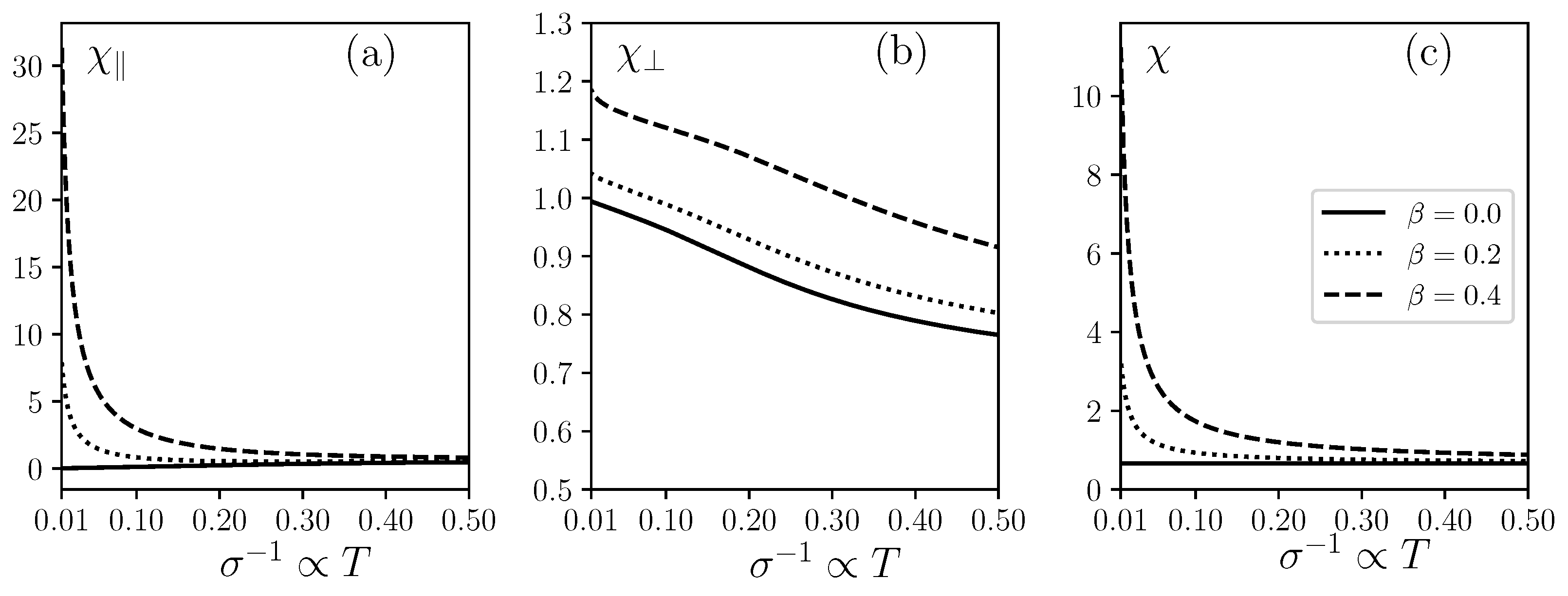
As is seen, for an AFM particle with fully compensated sublattice magnetizations ($\beta =0$), this formula reduces to just its first term.

It is useful to present ${\chi }_{\Vert }$ for the cases of low ($\sigma \gg 1$) and high ($\sigma \ll 1$) temperatures. The pertinent expansions for function $R^{\prime }\left(\sigma \right)/R\left(\sigma \right)$ were derived in [20]:

$$\frac{R^{\prime }\left(\sigma \right)}{R\left(\sigma \right)}=1-\frac{1}{\sigma }-\frac{1}{2{\sigma }^2}+\dots ,(\sigma \gg 1);\frac{R^{\prime }\left(\sigma \right)}{R\left(\sigma \right)}=\frac{1}{3}·\left(1+\frac{4\sigma }{15}+\frac{8{\sigma }^2}{315}+\dots \right),(\sigma \ll 1).$$

With this asymptotics, one obtains

$${\chi }_{\Vert }=\left\{\begin{array}{cc}\frac{1}{\sigma }+2{\beta }^2\left(\sigma -\frac{1}{2\sigma }\right),\hfill & \hfill \mathrm{for}\sigma \gg 1,\\ \frac{2}{3}\left[1+\sigma \left({\beta }^2-\frac{2}{15}\right)\right],\hfill & \hfill \mathrm{for}\sigma \ll 1.\end{array}\right.$$

(33)

Equation (33) shows that in the low-temperature limit $T\to 0$ ($\sigma \to \infty$), the susceptibility ${\chi }_{\Vert }$ tends to zero in the particles with full magnetic compensation ($\beta =0$) and grows boundlessly provided $\beta \ne 0$. In the high-temperature ($\sigma \to 0$) range, ${\chi }_{\Vert }$ tends to a constant value $2/3$ whatever the decompensation parameter. The plots of Figure 1a illustrate this behavior.

3.2. Static Susceptibility in Perpendicular Field

In the transverse configuration, where the external field is perpendicular to the anisotropy axis, the energy function scaled with the thermal energy writes

$${\mathcal{U}}_m(\vartheta ,\phi )/T=-2\beta \sigma qsin\vartheta cos\phi +\sigma q^2\left({sin}^2\vartheta {cos}^2\phi \right)-\sigma {cos}^2\vartheta ,$$

with $\vartheta$ and $\phi$ being the polar and azimuth angles defining the orientation of the AFM vector $\mathit{e}$; we remind that the polar axis points along the anisotropy one. In this case, the projection of nondimensional magnetization in the field direction takes the form

$$\mathfrak{m}=\beta \langle sin\vartheta cos\phi \rangle +q\left(1-\langle {sin}^2\vartheta {cos}^2\phi \rangle \right).$$

(34)

To find the linear susceptibility, we expand it to the first order in the field strength. The mean value of the product $sin\vartheta cos\phi$, evaluated with that accuracy, is

$$\begin{array}{c}\langle sin\vartheta cos\phi \rangle =\frac{1}{4\pi R\left(\sigma \right)}\underset{0}{\overset{\pi }{\int }}d\vartheta ·{sin}^2\vartheta exp\left(\sigma {cos}^2\vartheta \right)\underset{0}{\overset{2\pi }{\int }}d\phi ·\left(1+2\beta \sigma qsin\vartheta cos\phi \right)cos\phi \hfill \\ \hfill =\frac{\beta \sigma q}{2\pi R\left(\sigma \right)}\underset{0}{\overset{\pi }{\int }}d\vartheta ·{sin}^3\vartheta exp\left(\sigma {cos}^2\vartheta \right)\underset{0}{\overset{2\pi }{\int }}d\phi {cos}^2\phi =\beta \sigma q\left[1-\frac{R^{\prime }\left(\sigma \right)}{R\left(\sigma \right)}\right],\end{array}$$

whereas for $\langle {sin}^2\vartheta {cos}^2\phi \rangle$, it suffices to find it in the zeroth approximation:

$$\begin{array}{c}\hfill \langle {sin}^2\vartheta {cos}^2\phi \rangle =\frac{1}{4\pi R\left(\sigma \right)}\underset{0}{\overset{\pi }{\int }}d\vartheta ·{sin}^3\vartheta exp\left(\sigma {cos}^2\vartheta \right)\underset{0}{\overset{2\pi }{\int }}d\phi ·{cos}^2\phi =\frac{1}{2}\left[1-\frac{R^{\prime }\left(\sigma \right)}{R\left(\sigma \right)}\right].\end{array}$$

With the aid of these expressions, the magnetization induced by the perpendicular field takes the form

$$\mathfrak{m}={\beta }^2\sigma q\left[1-\frac{R^{\prime }\left(\sigma \right)}{R\left(\sigma \right)}\right]+q\left[1-\frac{1}{2}\left(1-\frac{R^{\prime }\left(\sigma \right)}{R\left(\sigma \right)}\right)\right],$$

(35)

so that the transverse susceptibility is

$${\chi }_{\perp }=\frac{1}{2}\left[1+\frac{R^{\prime }\left(\sigma \right)}{R\left(\sigma \right)}\right]+\sigma {\beta }^2\left[1-\frac{R^{\prime }\left(\sigma \right)}{R\left(\sigma \right)}\right]$$

(36)

with the following asymptotic expressions obtained for it with the aid of Formulas (33):

$${\chi }_{\perp }=\left\{\begin{array}{cc}1+{\beta }^2-\frac{1}{2\sigma }(1-{\beta }^2),\hfill & \hfill \mathrm{for}\sigma \gg 1,\\ \frac{2}{3}\left[1+\sigma \left({\beta }^2+\frac{1}{15}\right)\right],\hfill & \hfill \mathrm{for}\sigma \ll 1.\end{array}\right.$$

(37)

In the athermal limit ($\sigma \to \infty$), the transverse susceptibility, as is seen from Equation (37), equals $1+{\beta }^2$.

The temperature behavior of ${\chi }_{\perp }$ is illustrated in Figure 1b. It is seen that the transverse susceptibility goes down with temperature at any value of the decompensation parameter $\beta$; however, this decay is not very fast.

3.3. Ensemble of Particles with Random Axes’ Orientation

The susceptibility of an ensemble of particles with an arbitrary distribution of the anisotropy axes’ orientations is obtained by averaging Formula (28) with a given distribution function of the orientation angle:

$$\chi ={\chi }_{\Vert }\overline{{cos}^2\psi }+{\chi }_{\perp }\overline{{sin}^2\psi },$$

where the overline denotes the angular, not statistical ensemble, averaging. An instructive example is the situation where this distribution is random, i.e., the axes are spread uniformly over the whole spatial angle. In that case, $\overline{{cos}^2\psi }=1/3$ and $\overline{{sin}^2\psi }=2/3$, so that the ensemble susceptibility simplifies to

$$\chi =\frac{1}{3}\left({\chi }_{\Vert }+2{\chi }_{\perp }\right),$$

and, after substitution of Expressions (32) and (36), takes the form

$$\chi =\frac{2}{3}\left(1+\sigma {\beta }^2\right).$$

(38)

Going back to the susceptibility defined in terms of dimensional quantities, one obtains

$${\chi }_H=\frac{\varphi }{\mathsf{\Lambda }}·\chi =\frac{1}{3}\varphi \left(\frac{2}{\mathsf{\Lambda }}+\frac{M_u^{2}V}{T}\right).$$

(39)

Being a combination of Equations (32) and (36), Formula (39) comprises two qualitatively different contributions. The first one depends neither on magnetic decompensation, nor on temperature; it renders the result of the relative inclination of the sublattices due to the applied field. The second one is the superparamagnetic origin: it is non-zero only if the AFM particles possess a non-compensated magnetic moment; this part goes down with the temperature increase. As expected, this part coincides with the susceptibility of an assembly of imaginary identical ferromagnetic particles with volume V and permanent magnetization $M_u$. As it should be in the case where the easy axes’ distribution is random, the linear static susceptibility of the ensemble does not depend on the magnetic anisotropy of the particles. The plots of Figure 1c illustrate these conclusions. The evident close resemblance of Figure 1a,c is due to the relatively small reference values of the transverse susceptibility ${\chi }_{\perp }$; see Figure 1b.

4. Dynamic Susceptibility

4.1. Kinetic Equation

The assumption that both the applied and intrinsic anisotropy field strengths are far lower than that of the exchange one facilitates substantially the problem of the dynamic response of an antiferromagnet. Then, the magnetic relaxation process in an AFM particle may be treated as a sequence of two stages, which differ greatly in their time scales. Initially, under the dominating effect of the exchange field during a short time ${\tau }_E$, the coherence of sublattice magnetizations is established: settling antiparallelly, they fix the length of the AFM vector ${\mathit{L}}_p$. The reference scale of this process may be associated with the decay time of the Larmor precession of magnetization of either of the sublattices in the exchange field $H_E$, viz. ${\tau }_E\sim {\left(\alpha \gamma \mathsf{\Lambda }{M}_0\right)}^{-1}$, where $\alpha$ is the “friction” coefficient and $\gamma$ the gyromagnetic ratio. For typical antiferromagnets with $H_E\sim {10}^5$–${10}^6$ Oe, this yields ${\tau }_E\sim {10}^{-13}$ s. Evidently, the same time lapse is required to establish a time-independent (20) link between the AFM vector and particle non-compensated magnetization The second stage of relaxation is a relatively slow decaying precession of the antiferromagnetic vector about the effective field, which is a superposition of the applied and anisotropy fields.

Therefore, over the intervals, which notably exceed ${\tau }_E$, the AFM vector rotates, keeping its length constant. Given the precessional character of this motion, if describing it phenomenological, it seems reasonable to use an equation of the Landau–Lifshitz–Gilbert type:

$$\frac{d\mathit{L}}{dt}=-\gamma \mathit{N}+\frac{\alpha }{L}\mathit{L}\times \frac{d\mathit{L}}{dt},$$

where $\mathit{N}$ is the effective magnetic torque; see Formula (18). As already mentioned, if neglecting corrections of the order of $\sim {(H/H_E)}^2$, the length of the AFM vector equals $2M_0$, so that this equation may be written for the unit vector $\mathit{e}$ as

$$\frac{d\mathit{e}}{dt}=\frac{\gamma }{2M_0}\left(\mathit{e}\times \frac{\partial U}{\partial \mathit{e}}\right)+\alpha \mathit{e}\times \frac{d\mathit{e}}{dt}.$$

(40)

To account for the orientational fluctuations of the AFM vector in nanoparticles, one has to transit from the deterministic Equation (40) to a kinetic equation of the Brown type for the distribution function $W(\mathit{e},t)$:

$$2{\tau }_D\frac{\partial W}{\partial t}={\widehat{\mathit{J}}}_{\mathit{e}}W{\widehat{\mathit{Q}}}_{\mathit{e}}\left(\frac{{\mathcal{U}}_m}{T}+lnW\right),{\widehat{\mathit{J}}}_{\mathit{e}}=\mathit{e}\times \frac{\partial }{\partial \mathit{e}},{\widehat{\mathit{Q}}}_{\mathit{e}}={\widehat{\mathit{J}}}_{\mathit{e}}+\frac{1}{\alpha }\frac{\partial }{\partial \mathit{e}}.$$

(41)

The relaxation time, herein introduced, defines the rate of rotary diffusion of the AFM vector in a particle with negligible magnetic anisotropy; for its estimate expression, ${\tau }_D=M_{0}V/\alpha \gamma T$, which follows from the fluctuation–dissipation theorem applied to Equation (41). However, in general, ${\tau }_D$ should be looked at as a phenomenological parameter deduced from the comparison of the theory with the experiment. It is worth noting that in the developed model, the time ${\tau }_D$ does not depend on the existence of non-compensated magnetization and, because of that, does not tend to zero when $M_u$ is absent in the particle. By that, our result differs essentially from the models developed in [17,18,19].

In the low-frequency interval (i.e., far below the microwave range), one may neglect in Equation (41) the probability flux that renders the precessional motion of vector $\mathit{e}$ and treat the magnetic response of the system as a purely relaxational one. A formal transition is performed by replacing in the kinetic Equation (42) operator ${\widehat{\mathit{Q}}}_{\mathit{e}}$ with ${\widehat{\mathit{J}}}_{\mathit{e}}$; the modified equation takes the form

$$2{\tau }_D\frac{\partial W}{\partial t}={\widehat{\mathit{J}}}_{\mathit{e}}W{\widehat{\mathit{J}}}_{\mathit{e}}\left(\frac{{\mathcal{U}}_m}{T}+lnW\right).$$

(42)

Note that the function W refers to the orientation distribution of the antiferromagnetic vector $\mathit{l}$, not the uncompensated magnetic moment ${\mathbf{\mu }}_u$, although in the developed model, they are always parallel. Therefore, Equation (42) is equally applicable to fully compensated AMF nanoparticles like those considered in [8]. An equation of that type was used in [21], where only the longitudinal response of AFM nanoparticles was investigated; herein, kinetic Equation (42) is used for the case of arbitrary field orientation. Assuming that the probing field is harmonic, the solution of Equation (42) is Fourier transformed, so that the sought after dynamic magnetic susceptibility is found from the linear relation $m_{\omega }=\chi \left(\omega \right)q_{\omega }$ between the Fourier components of the statistically averaged nondimensional magnetization and field. Repeating for the case of the AC field the considerations that led to Expression (28), one comes to the relation

$$\chi \left(\omega \right)={\chi }_{\Vert }\left(\omega \right){cos}^2\psi +{\chi }_{\perp }\left(\omega \right){sin}^2\psi ,$$

(43)

where indices mark the susceptibility components for the cases of the probing field being directed either along or across the particle anisotropy axis.

4.2. Longitudinal Dynamic Susceptibility

The expression for the longitudinal dynamic susceptibility of a nanosized AFM particle with a non-compensated magnetization was obtained in [21]. In brief, this was performed as follows. The solution of Equation (42) is constructed in the Gilbert functional space, whose unit vectors are spherical harmonics

$$Y_{l,k}(\vartheta ,\phi )={(-1)}^k\sqrt{\frac{(2l+1)(l-k)!}{4\pi (l+k)!}}{P}_{l,k}(cos\vartheta ){\mathit{e}}^{ik\phi },-l\le k\le l,Y_{l,k}^{*}={(-1)}^k{Y}_{l,-k},$$

(44)

which constitute a canonical basis of rotational group representation in 3D space. For the case $U/T\to 0$, they are eigenfunctions of the coordinate part of the operator of the kinetic Equation (43). If $\mathit{h}\Vert \mathit{n}$, distribution function W depends only on the angle $\vartheta$ that AFM vector $\mathit{e}$ makes with the anisotropy axis, so that expansion:

$$W(\vartheta ,t)=\sum _{l=0}^{l=\infty }{b}_l\left(t\right)Y_{l,0}\left(\vartheta \right)$$

comprises only spherical harmonics (44) with $k=0$. Substituting this series in (42), one arrives at the set of linear equations for coefficients $b_l$:

$$\begin{array}{c}\frac{{\tau }_0}{l(l+1)}\frac{d{b}_l}{dt}=\left(\frac{1-q^2}{(2l-1)(2l+3)}-\frac{1}{2\sigma }\right)b_l+\frac{1}{2}\beta q\left(\sqrt{\frac{1}{(2l-1)(2l+1)}}{b}_{l-1}-\sqrt{\frac{1}{(2l+1)(2l+3)}}{b}_{l+1}\right)\hfill \\ \hfill +(1-q^2)\left(\frac{l-1}{2l-1}\sqrt{\frac{1}{(2l-3)(2l+1)}}{b}_{l-2}-\frac{l+2}{2l+3}\sqrt{\frac{1}{(2l+1)(2l+5)}}{b}_{l+2}\right),\end{array}$$

with the reference time ${\tau }_0={\tau }_D/\sigma =M_0/\left(\alpha \gamma K\right)$, which in this representation, is both temperature- and particle-size-independent In the superparamagnetic theory, the ratio $f_0=1/\left(2\pi {\tau }_0\right)$ is usually identified with the so-called attempt frequency, which characterizes oscillations of the magnetic moment inside the potential well imposed on it by the anisotropy energy.

By introducing a column vector:

$$\mathit{X}=\left(\begin{array}{c}{b}_1\\ b_2\\ ⋮\\ b_N\end{array}\right),$$

this set of equations may be transformed to matrix form:

$${\tau }_0\frac{d\mathit{X}}{dt}=\mathbf{A}·\mathit{X}+\mathit{B}.$$

(45)

The number N of elements is chosen on the requirement that, upon increasing it, the results would not change within the prescribed accuracy; the elements of the free term vector $\mathit{B}$ are proportional to coefficient $b_0=1/\sqrt{4\pi }$.

To find the susceptibility, Equation (45) is linearized. For that, the to-be-evaluated vector $\mathit{X}$ is presented as the sum of equilibrium components ${\mathit{X}}_0$; it corresponds to zero applied field ($q=0$) and a small non-equilibrium additive ${\mathit{X}}_1$. In the same approximation, matrix $\mathbf{A}$ and column vector $\mathit{B}$ are expanded as

$$\mathbf{A}={\mathbf{A}}_0+q{\mathbf{A}}_1,\mathit{B}={\mathit{B}}_0+q{\mathit{B}}_1;$$

here, ${\mathbf{A}}_0=\mathbf{A}(q=0)$ and ${\mathit{B}}_0=\mathit{B}(q=0)$ refer to the unperturbed state, whereas the non-equilibrium parts should be evaluated from the equation

$${\tau }_0\frac{d{\mathit{X}}_1}{dt}={\mathbf{A}}_0·{\mathit{X}}_1+q\left({\mathbf{A}}_1·{\mathit{X}}_0+B_1\right).$$

At a short time lapse, its solution is

$${\mathit{X}}_1(t+dt)=\sum _{k=1}^{\infty }{\alpha }_k{\mathit{V}}_k{\mathit{e}}^{-{\lambda }_k^{0}dt}+{\tilde{\mathit{X}}}_1,$$

where ${\mathit{V}}_k$ and ${\lambda }_k^0$ are the eigenvectors and absolute values of eigenvalues of matrix ${\mathbf{A}}_0$; the terms in this sum are settled in ascending order with respect to ${\lambda }_k^0$. At the time interval $dt$, vector

$${\tilde{\mathit{X}}}_1=-q\mathit{F},\mathit{F}={\mathbf{A}}_0^{-1}·({\mathbf{A}}_1·{\mathit{X}}_0+{\mathit{B}}_1)$$

(46)

yields a constant contribution to the solution.

In [21], it is shown that the smallest eigenvalue of unperturbed matrix ${\mathbf{A}}_0$ is

$${\lambda }_1^0=\frac{1}{{\tau }_0}\sqrt{\frac{4\sigma }{\pi }}{e}^{-\sigma },\sigma =\frac{KV}{T}.$$

(47)

As the temperature parameter $\sigma$ grows, ${\lambda }_1^0$ goes down exponentially and at $\sigma \gtrsim 1$ becomes far smaller than any of the other eigenvalues ${\lambda }_k^0$. This enables one to proceed to a more rough time scale, where the time lapses $dt\gg 1/{\lambda }_k^0$ for any $k⩾2$, so that the system response becomes a single-mode one:

$${\mathit{X}}_1(t+dt)={\alpha }_1{\mathit{V}}_1{\mathit{e}}^{-{\lambda }_1^0·dt}+{\tilde{\mathit{X}}}_1,$$

and the equation for the non-equilibrium additive simplifies to

$$\frac{d{\mathit{X}}_1\left(t\right)}{dt}=-{\lambda }_1^0\left[{\mathit{X}}_1\left(t\right)-{\tilde{\mathit{X}}}_1\left(t\right)\right],$$

which leads to the following Fourier representation:

$${\mathit{X}}_1^{\omega }=\frac{{\tilde{\mathit{X}}}_1^{\omega }}{1+i\omega {\tau }_1}=\frac{\mathit{F}}{1+i\omega {\tau }_1}{q}_{\omega },{\tau }_1=1/{\lambda }_1^0.$$

(48)

In terms of the components of vector $\mathit{X}$, the nondimensional ensemble magnetization (23) is expressed as

$$\mathfrak{m}\left(t\right)=\beta \langle cos\vartheta \rangle +q\left[1-\langle {cos}^2\vartheta \rangle \right]=\sqrt{\frac{4\pi }{3}}\beta b_1\left(t\right)+q\left(\frac{2}{3}-\sqrt{\frac{16\pi }{45}}\right)b_2\left(t\right).$$

(49)

Performing Fourier transformation, one obtains

$${\mathfrak{m}}_{\omega }=\sqrt{\frac{4\pi }{3}}\beta b_1^{\omega }+\left(\frac{2}{3}-\sqrt{\frac{16\pi }{45}}{b}_2^0\right)q_{\omega }.$$

(50)

In this formula, $b_1^{\omega }$ is the first element of vector ${\mathit{X}}_1^{\omega }$, whereas $b_2^0$ equals the equilibrium value of coefficient $b_2$ under zero field, making the second element of vector ${\mathit{X}}_0$. With the allowance of the representation (49) for ${\mathit{X}}_1^{\omega }$ and for the frequency independence of vector ${\mathit{X}}_0$, Expression (50) may be transformed to ${\mathfrak{m}}_{\omega }={\chi }_{\Vert }·q_{\omega }$, where

$${\chi }_{\Vert }\left(\omega \right)={\chi }_{\Vert }^{\left(0\right)}+\frac{{\chi }_{\Vert }^{\left(1\right)}}{1+i\omega {\tau }_1}.$$

(51)

The frequency-independent term ${\chi }_{\Vert }^{\left(0\right)}$ in the susceptibility expression (51) is

$${\chi }_{\Vert }^{\left(0\right)}=\frac{2}{3}-\sqrt{\frac{16\pi }{45}}{b}_2^0=1-{\langle {cos}^2\vartheta \rangle }_0=1-\frac{R^{\prime }\left(\sigma \right)}{R\left(\sigma \right)};$$

(52)

it does not depend on decompensation parameter $\beta$ and delivers the susceptibility of a fully compensated antiferromagnet. As Equation (52) shows, the frequency dependence of the magnetic response of an AFM particle is of the Debye type. Therefore, at $\omega =0$, the sum of ${\chi }_{\Vert }^{\left(0\right)}+{\chi }_{\Vert }^{\left(1\right)}$ should reduce to the longitudinal static susceptibility (32). Given that, one finds that the Debye (dispersion) part of Equation (50) depends quadratically on decompensation parameter $\beta$:

$${\chi }_{\Vert }^{\left(1\right)}=2{\beta }^2\sigma ·\frac{R^{\prime }\left(\sigma \right)}{R\left(\sigma \right)}.$$

(53)

4.3. Arbitrary Orientation of Anisotropy Axes

As the previously presented results show, to evaluate the dynamic susceptibility in the single-mode approximation, it suffices to find the static components and—for determining the frequency dependence—to know the lowest (by its modulus) eigenvalue of the unperturbed kinetic matrix. If the system is subject only to a probing field (no permanent bias), then the mentioned eigenvalue is delivered by Formula (47) and is independent of the particle orientation. Following this pattern, the transverse dynamic susceptibility of an AFM nanoparticle may be presented as

$${\chi }_{\perp }\left(\omega \right)={\chi }_{\perp }^{\left(0\right)}+\frac{{\chi }_{\perp }^{\left(1\right)}}{1+i\omega {\tau }_1},\mathrm{where}{\tau }_1={\tau }_0·\sqrt{\frac{\pi }{4\sigma }}{e}^{\sigma }.$$

(54)

The frequency-independent term ${\chi }_{\perp }^{\left(0\right)}$ is the static susceptibility of a magnetically compensated particle; according to Equation (36), it is

$${\chi }_{\perp }^{\left(0\right)}=\frac{1}{2}\left(1+\frac{R^{\prime }\left(\sigma \right)}{R\left(\sigma \right)}\right).$$

(55)

The difference between the static transverse susceptibilities of non-compensated and compensated (55) particles yields the coefficient of the dispersion term in (54):

$${\chi }_{\perp }^{\left(1\right)}=\sigma {\beta }^2\left(1-\frac{R^{\prime }\left(\sigma \right)}{R\left(\sigma \right)}\right).$$

(56)

The above-obtained expressions for the longitudinal and transverse components and Formula (43) enable one to find the linear magnetic response of an AFM particle at an arbitrary inclination of the probing field to the anisotropy axis. Besides that, averaging Equation (43) over a given distribution function of $\psi$ yields the susceptibility of an ensemble of those particles with any prescribed orientational texture. In particular, if the axes are distributed at random, so that $\overline{{cos}^2\psi }=1/3$, the dynamic susceptibility is rendered by the expression

$$\chi \left(\omega \right)=\frac{2}{3}\left[1+\frac{\sigma {\beta }^2}{1+i\omega {\tau }_1}\right].$$

(57)

5. Discussion

The most probable orientation texture of a solid ensemble of AFM nanoparticles, given the low if any values of the particle magnetic moments, is the random one, in whichever way the system is prepared: by solidification of a colloid or by phase separation in a solid solution. In principle, this applies even to a true (liquid) colloid if there are no non-magnetic (e.g., chemical) sources of the particle structuring. Then, from the experimental viewpoint, the susceptibility of type (57) seems to be the subject of prime interest.

As follows from the problem formulation, herein, we addressed only the low-frequency dynamics of the AFM particles, setting aside the processes in the Larmor frequency range. Because of that, in our model, the susceptibility components come out as simple analytical formulas. In particular, the orientation-averaged function (57) that characterizes a random system comes out as two-term expression that combines the constant contribution due to the exchange coupling of the sublattices and a temperature-dependent term entailed by the presence of the uncompensated magnetization.

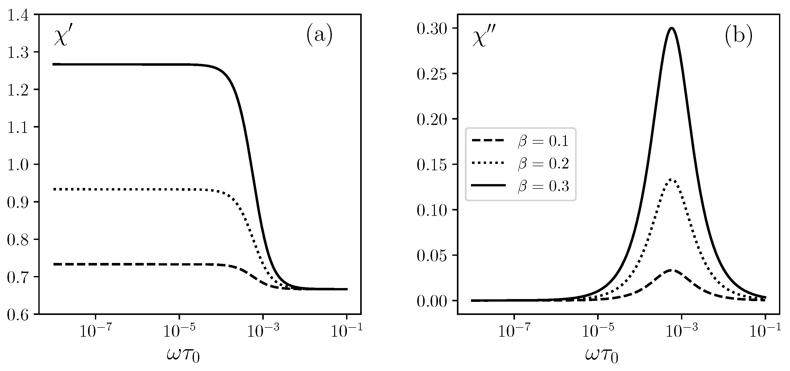
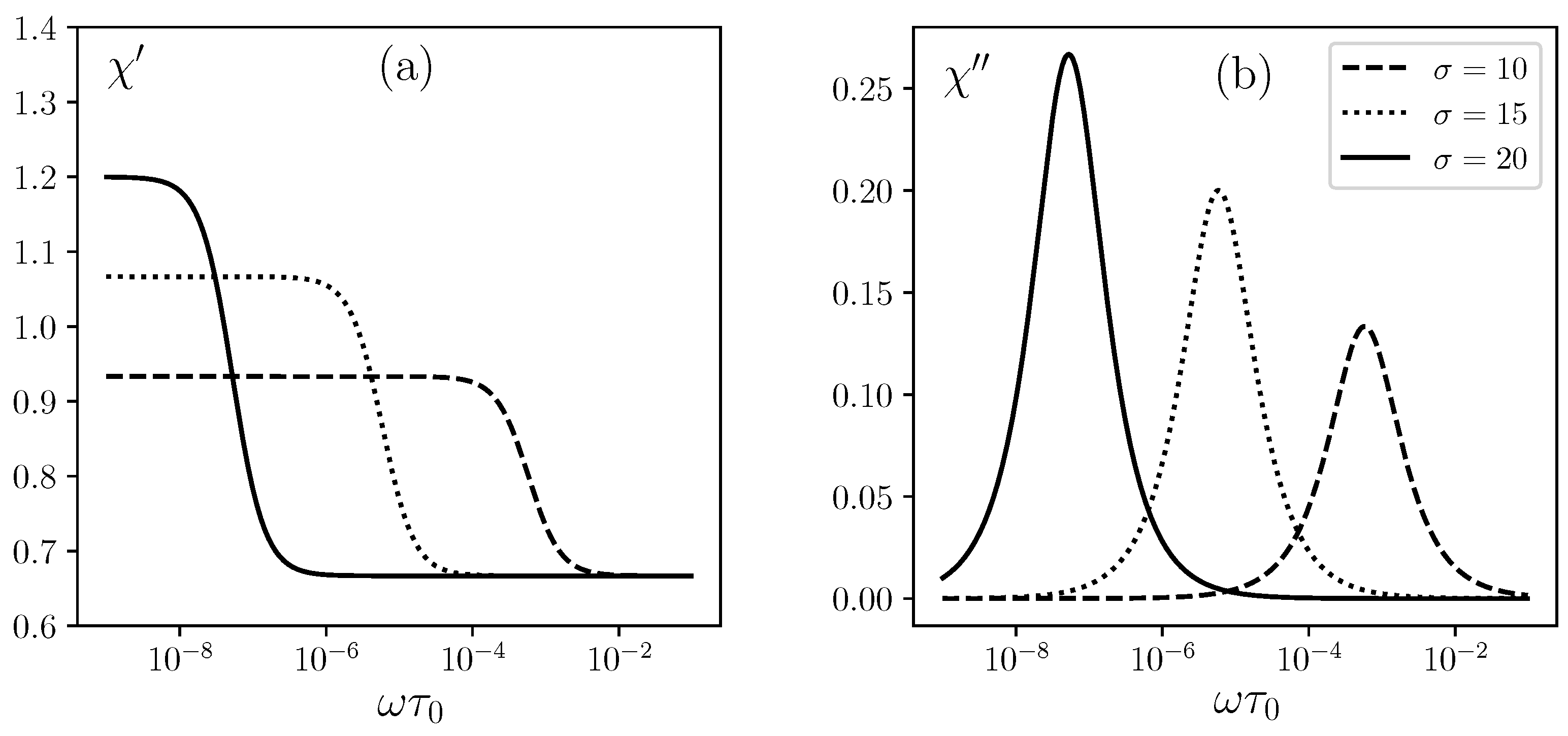
Formula (57) contains just one relaxation time, and because of that, the modeled frequency dependences of the in-phase and out-phase components of the dynamic susceptibility (see Figure 2 and Figure 3) have a Debye-like shape.

The only difference is that the exchange contribution, which within the envisioned temperature and field-amplitude intervals, is considered as a constant, yields some pedestal for those otherwise standard Debye lines. The temperature dependence of the absorption line is in full compliance with the superparamagnetic behavior: with cooling, the peak shifts to lower frequencies; see Figure 3. In general, with allowance for the unavoidable polydispersity of the nanoparticles, this conclusion fairly well complies with the temperature dependences of the AC susceptibility of ferritins reported in [10,14,15].

The mentioned temperature drift of the absorption peak is inherent, as such, to all the models based on the superparamagnetic approach. For example, in the model developed in [17,18,19], where a single AFM particle with the anisotropy axis tilted to the applied field under some fixed angle was considered, the overall temperature behavior of the susceptibility components is essentially the same.

The difference between the above-presented results and those of [17,18,19] is conceptual and stems from the statement of the kinetic problem. Our Equation (41) describes the stochastic motion of antiferromagnetic vector $\mathit{l}$, which is the characteristic of any AFM particle whether or not it bears an uncompensated magnetic moment ${\mathit{m}}_u$. Therefore, the latter is albeit an important, but optional attribute of an AFM particle. We remark that, in [8], where fully compensated AFM nanoparticles were considered without using the kinetic equation, the model fundamentally implies that ${\tau }_0$ is taken to be proportional to $M_0$. Meanwhile, the kinetic equation on which the considerations of [17,18,19] were based employs only the orientation distribution function of the uncompensated magnetic moment as itself. Because of that, the latter description seems to come to a dead-end as soon as the particle magnetic moment goes down to ${\mathit{m}}_u=0$.

The difference in the approaches entails a qualitative mismatch in the time scales of the respective models. This is clear if comparing the definitions, the one given in the above and its analogue, which follows from Formula (3) of [17]. Presenting them in temperature-independent form, one obtains

$${\tau }_0={\tau }_D/\sigma =M_0/\alpha \gamma K,{\tau }_0^{*}={\tau }_N/\sigma =M_u/\alpha \gamma K.$$

(58)

As is seen, the attempt time ${\tau }_0$ does not depend on the uncompensated magnetization, whereas ${\tau }_0^{*}$ diverges at $M_u\to 0$, i.e., when the AFM particle loses its magnetic moment, remaining intact otherwise. This looks to be an unphysical effect.

Unfortunately, the experimental evidence reported in [10,14,15] is insufficient to be used for a decisive choice between the models. The crucial point is that the estimated values of ${\tau }_0$ (or ${\tau }_0^{*}$) for the AFM nanoparticle samples tested there vary from ${10}^{-12}$ to ${10}^{-9}$ s. This is a general issue: until now, the evaluation of the attempt time is a “weak point” in superparamagnetic theory. Such an evaluation goes via determining the blocking temperature $T_B$, which is usually identified with the position of the cusp of ZFC magnetization curves. As shown in [22], this method, besides being strongly affected by the polydispersity of the sample, is nevertheless acceptable in the case of ferromagnetic nanoparticles, but may cause huge errors if applied—as was done in [10,14,15]—to AFM nanoparticles with ${\mathbf{\mu }}_u$. Due to that, one has to admit that the uncertainty in the evaluation of ${\tau }_0$ remains huge even if the particle volume and ${\mathbf{\mu }}_u$ are well known.

A direct way to compare the model predictions would have been to make a set of AC measurements on a number of otherwise identical nanoparticles differing just by the value of their uncompensated magnetic moments. As far as we know, no such attempts have been made so far. Although, the task of preparing such samples seems to pose a serious problem, this does not mean that it is impossible in principle. For example, the technique of synthesizing artificial ferritins that enables one to modify the iron-containing core of the apoferritin protein cage [23,24] might offer a plausible solution.

6. Conclusions

A kinetic model of low-frequency magnetic susceptibility for antiferromagnetic nanoparticles bearing uncompensated magnetic moments was developed. In this frequency domain, the exchange interaction maintains a strong correlation (anti-parallelism) of the sublattice magnetizations, thus forming the antiferromagnetic vector $\mathit{L}$ of constant length. The permanent (uncompensated) magnetic moment ${\mathbf{\mu }}_u$ entailed by the nanosize of the particle comes out as a result of the difference between those magnetizations. Due to that, in equilibrium vectors ${\mathbf{\mu }}_u$ and $\mathit{L}$ are always coaligned. The kinetic equation that describes the effect of thermal fluctuations on the particle magnetodynamics is formulated for the motion of $\mathit{L}$, so that the magnetic response is an optional result of decompensation. The orientation relaxation time is proportional to the sublattice magnetization and refers equally to the rotary relaxation of $\mathit{L}$ and ${\mathbf{\mu }}_u$.

References

1. Néel, L. Superparamagnétisme des graines très fins antiferromagnétiques. C. R. Acad. Sci. 1961, 252, 4075–4080. [Google Scholar]
2. Néel, L. Superposition de l’antiferromagnétisme et du superparamagnétisme dans un graine très fin. C. R. Acad. Sci. 1961, 253, 9–12. [Google Scholar]
3. Baltz, V.; Manchon, A.; Tsoi, M.; Moriyama, T.; Ono, T.; Tserkovnyak, Y. Antiferromagnetic spintronics. Rev. Mod. Phys. 2018, 90, 015005. [Google Scholar] [CrossRef] [Green Version]
4. Peng, Y.-K.; Liu, C.-L.; Chen, H.-C.; Chou, S.-W.; Tseng, W.-H.; Tseng, Y.-J.; Kang, C.-C.; Hsiao, J.-K.; Chou, P.-T. Antiferromagnetic iron nanocolloids: A new generation in vivo T1 MRI contrast agent. J. Am. Chem. Soc. 2013, 135, 18621–18628. [Google Scholar] [CrossRef]
5. Tang, Z.; Zhang, H.; Liu, Y.; Ni, D.; Zhang, H.; Zhang, J.; Yao, Z.; He, M.; Shi, J.; Bu, W. Antiferromagnetic pyrite as the tumor microenvironment-mediated nanoplatform for self-enhanced tumor imaging and therapy. Adv. Mater. 2016, 19, 1701683. [Google Scholar] [CrossRef]
6. Neves, H.R.; Bini, R.A.; Barbosa, J.H.O.; Salmon, C.G.; Varanda, L.C. Dextran-coated antiferromagnetic MnO nanoparticles for a T1 MRI contrast agent with high colloidal stability. Part. Part. Syst. Charact. 2016, 33, 167–176. [Google Scholar] [CrossRef]
7. Kannan, K.; Radhika, D.; Nikolova, N.P.; Sadasivuni, K.K.; Mahdizadeh, H.; Verma, U. Structural studies of bio-mediated NiO nanoparticles for photocatalytic and antibacterial activities. Inorg. Chem. Commun. 2020, 113, 107755. [Google Scholar] [CrossRef]
8. Rózsa, L.; Selzer, S.; Birk, T.; Atxitia, U.; Nowak, U. Reduced thermal stability of antiferromagnetic nanostructures. Phys. Rev. B 2019, 100, 064422. [Google Scholar] [CrossRef] [Green Version]
9. Richardson, J.T.; Yiagas, D.I.; Turk, B.; Forster, K.; Twigg, M.V. Origin of superparamagnetism in nickel oxide. J. Appl. Phys. 1991, 70, 6977–6982. [Google Scholar] [CrossRef]
10. Kilcoyne, S.H.; Cywinski, R. Ferritin: A model superparamagnet. J. Magn. Magn. Mater. 1995, 140–144, 1466–1467. [Google Scholar] [CrossRef]
11. Iimori, T.; Imamoto, Y.; Uchida, N.; Kikuchi, Y.; Honda, K.; Iwahashi, T.; Ouchi, Y. Magnetic moment distribution in nanosized antiferromagnetic NiO. J. Appl. Phys. 2020, 127, 023902. [Google Scholar] [CrossRef]
12. Balaev, D.A.; Krasikov, A.A.; Dubrovskiy, A.A.; Popkov, S.I.; Stolyar, S.V.; Bayukov, O.A.; Iskhakov, R.S.; Ladygina, V.P.; Yaroslavtsev, R.N. Magnetic properties of heat treated bacterial ferrihydrite nanoparticles. J. Magn. Magn. Mater. 2016, 410, 171–180. [Google Scholar] [CrossRef]
13. Balaev, D.A.; Krasikov, A.A.; Popkov, S.I.; Dubrovskiy, A.A.; Semenov, S.V.; Velikanov, D.A.; Bayukov, O.A.; Kirillov, V.L.; Mart’yanov, O.N. Features of the quasi-static and dynamic magnetization switching in NiO nanoparticles: Manifestation of the interaction between magnetic subsystems in antiferromagnetic nanoparticles. J. Magn. Magn. Mater. 2020, 515, 167307. [Google Scholar] [CrossRef]
14. Allen, P.D.; St Pierre, T.G.; Chua-anusorn, W.; Ström, V.; Rao, K.V. Low-frequency low-field magnetic susceptibility of ferritin and hemosiderin. Biochim. Biophys. Acta 2000, 1500, 186–196. [Google Scholar] [CrossRef] [Green Version]
15. Guertin, R.P.; Harrison, N.; Zhou, Z.X.; McCall, S.; Drymiotis, F. Very high field magnetization and AC susceptibility of native horse spleen ferritin. J. Magn. Magn. Mater. 2007, 308, 97–100. [Google Scholar] [CrossRef]
16. Raikher, Y.L.; Stepanov, V.I. Magnetic relaxation in a suspension of antiferromagnetic nanoparticles. J. Exp. Theor. Phys. 2008, 107, 435–444. [Google Scholar] [CrossRef]
17. Ouari, B.; Aktaou, S.; Kalmykov, Y.P. Reversal time of the magnetization of antiferromagnetic nanoparticles. Phys. Rev. B 2010, 81, 024412. [Google Scholar] [CrossRef]
18. Ouari, B.; Kalmykov, Y.P. Effect of a dc bias magnetic field on the magnetization relaxation of antiferromagnetic nanoparticles. Phys. Rev. B 2011, 83, 064406. [Google Scholar] [CrossRef]
19. Kalmykov, Y.P.; Ouari, B.; Titov, S.V. Dynamic magnetic hysteresis and nonlinear susceptibility of antiferromagnetic nanoparticles. J. Appl. Phys. 2016, 120, 053901. [Google Scholar] [CrossRef]
20. Raikher, Y.L.; Shliomis, M.I. Theory of dispersion of magnetic susceptibility of fine ferromagnetic particles. J. Exp. Theor. Phys. 1975, 40, 526–532. [Google Scholar]
21. Poperechny, I. Longitudinal remagnetization of uniaxial antiferromagnetic nanoparticles: The role of spontaneous magnetic moment. Philos. Trans. R. Soc. Ser. A 2022, 380, 20200312. [Google Scholar] [CrossRef] [PubMed]
22. Madsen, D.E.; Hansen, M.F.; Mørup, S. The correlation between superparamagnetic blocking temperatures and peak temperatures obtained from ac magnetization measurements. J. Phys. C Condens. Matter 2007, 20, 345209. [Google Scholar] [CrossRef]
23. Yamashita, I.; Iwahori, K.; Kumagai, S. Ferritin in the field of nanodevices. Biochim. Biophys. Acta 2010, 1800, 846–857. [Google Scholar] [CrossRef] [PubMed]
24. Nandwana, V.; Ryoo, S.R.; Kanthala, S.; Kumar, A.; Sharma, A.; Castro, F.C.; Lia, Y.; Hoffman, B.; Lim, S.; Dravid, V.P. Engineered ferritin nanocages as natural contrast agents in magnetic resonance imaging. RSC Adv. 2017, 7, 34892–34900. [Google Scholar] [CrossRef]
Figure 1. Temperature dependence of the static magnetic susceptibilities of an ensemble of AFM particles whose anisotropy axes are: (a) parallel with the applied field, (b) perpendicular to it, and (c) distributed at random; the decompensation parameter β = 0 (solid lines), 0.2 (dots), 0.4 (dashes). Note the different vertical scales in all three panes.
Magnetism 02 00024 g001
Figure 2. Frequency dependence of the: (a) real χ and (b) imaginary χ parts of the magnetic susceptibility of an antiferromagnetic particle ensemble with a random distribution of the anisotropy axes; the decompensation parameter β is: 0.1 (dashes), 0.2 (dots), 0.3 (solid lines); the temperature parameter σ = 10 .
Magnetism 02 00024 g002
Figure 3. Frequency dependence of: (a) real χ and (b) imaginary χ parts of the magnetic susceptibility of an antiferromagnetic particle ensemble with a random distribution of the anisotropy axes; the temperature parameter σ is: 10 (dashes), 20 (dots), 30 (solid lines); the decompensation parameter β = 0.2 .
Magnetism 02 00024 g003
Publisher’s Note: MDPI stays neutral with regard to jurisdictional claims in published maps and institutional affiliations.