
Uncovering the Origins of Instability in Dynamical Systems: How Can the Attention Mechanism Help?

Abstract
:1. Introduction
2. Materials and Methods
2.1. Simulated Dynamical System
2.2. Attention Mechanism
2.2.1. First Module: Initial Node Feature Embedding
2.2.2. Second Module: Learnable Attention Mechanism
2.2.3. Third Module: Graph Convolution
2.2.4. Final Module: Backpropagation and Training
2.3. Spectral Stability Analysis
2.4. Topological Stability Analysis
2.5. Symmetry-Breaking Stability Analysis
2.6. Theoretical Justification for Analysis Approaches
3. Results
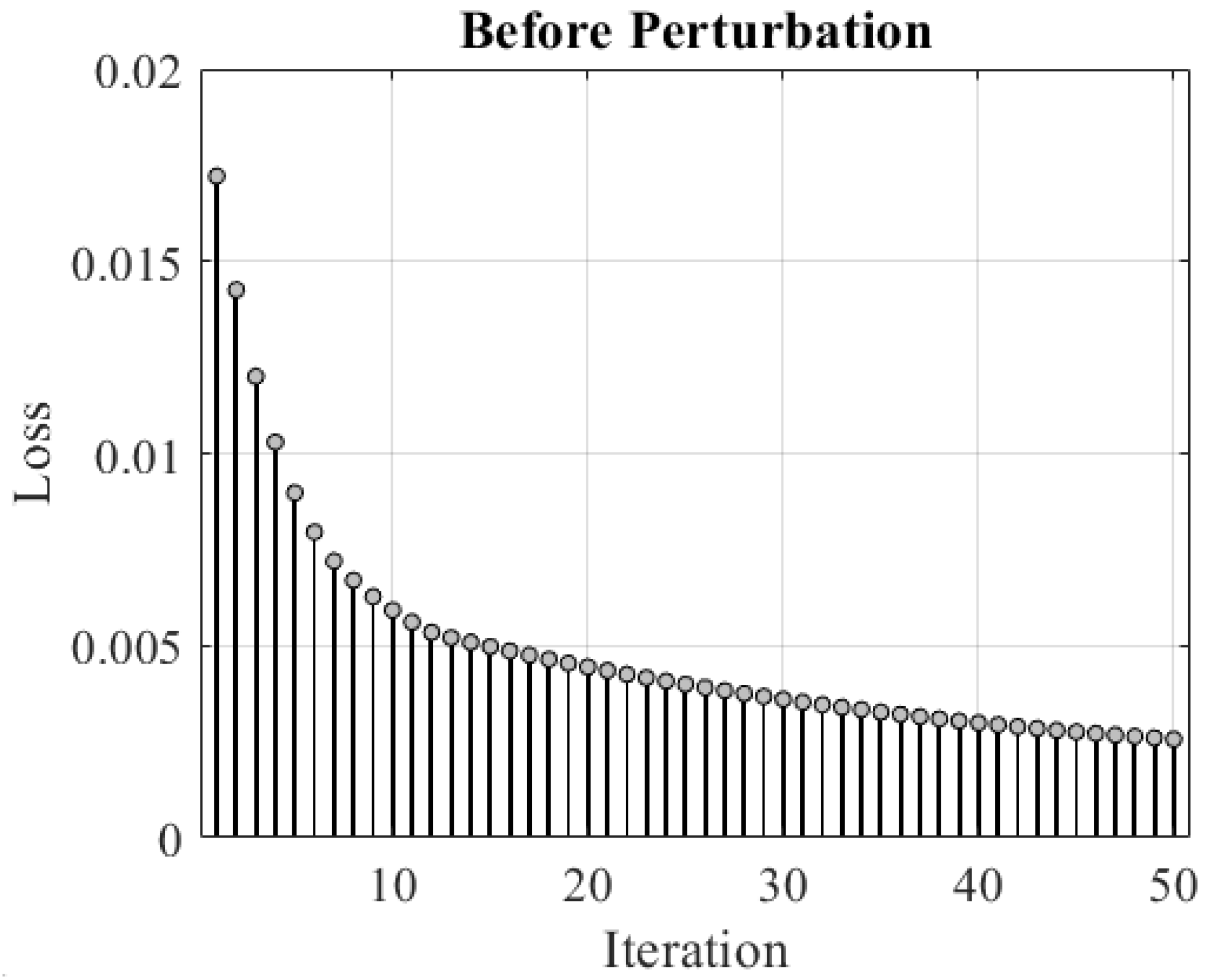
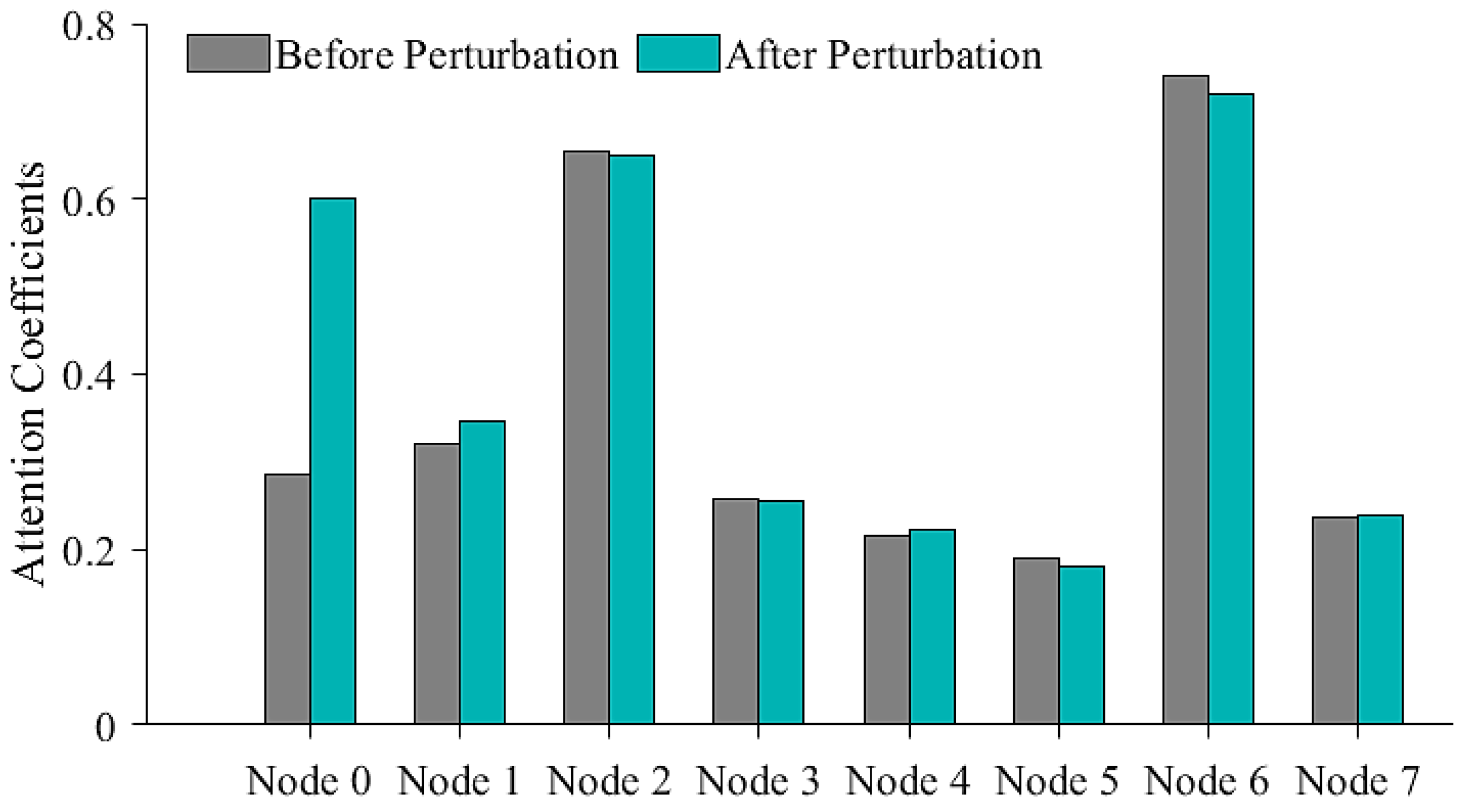
3.1. Attention Mechanism
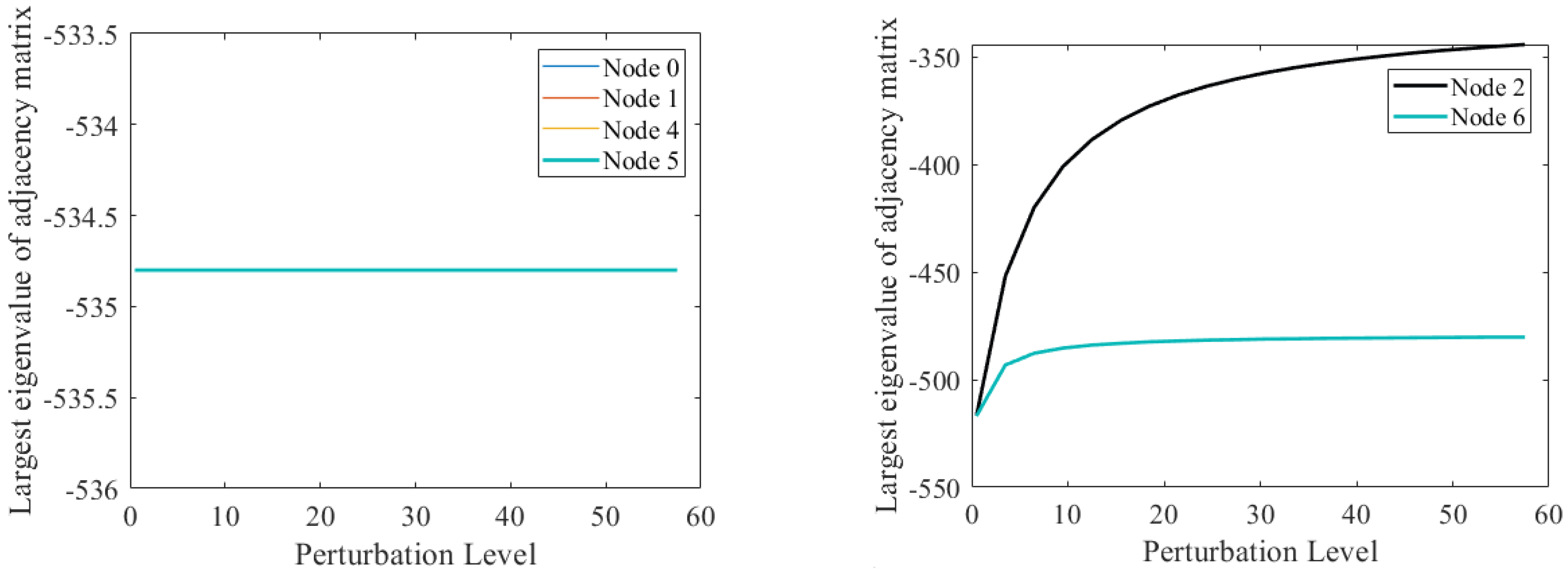
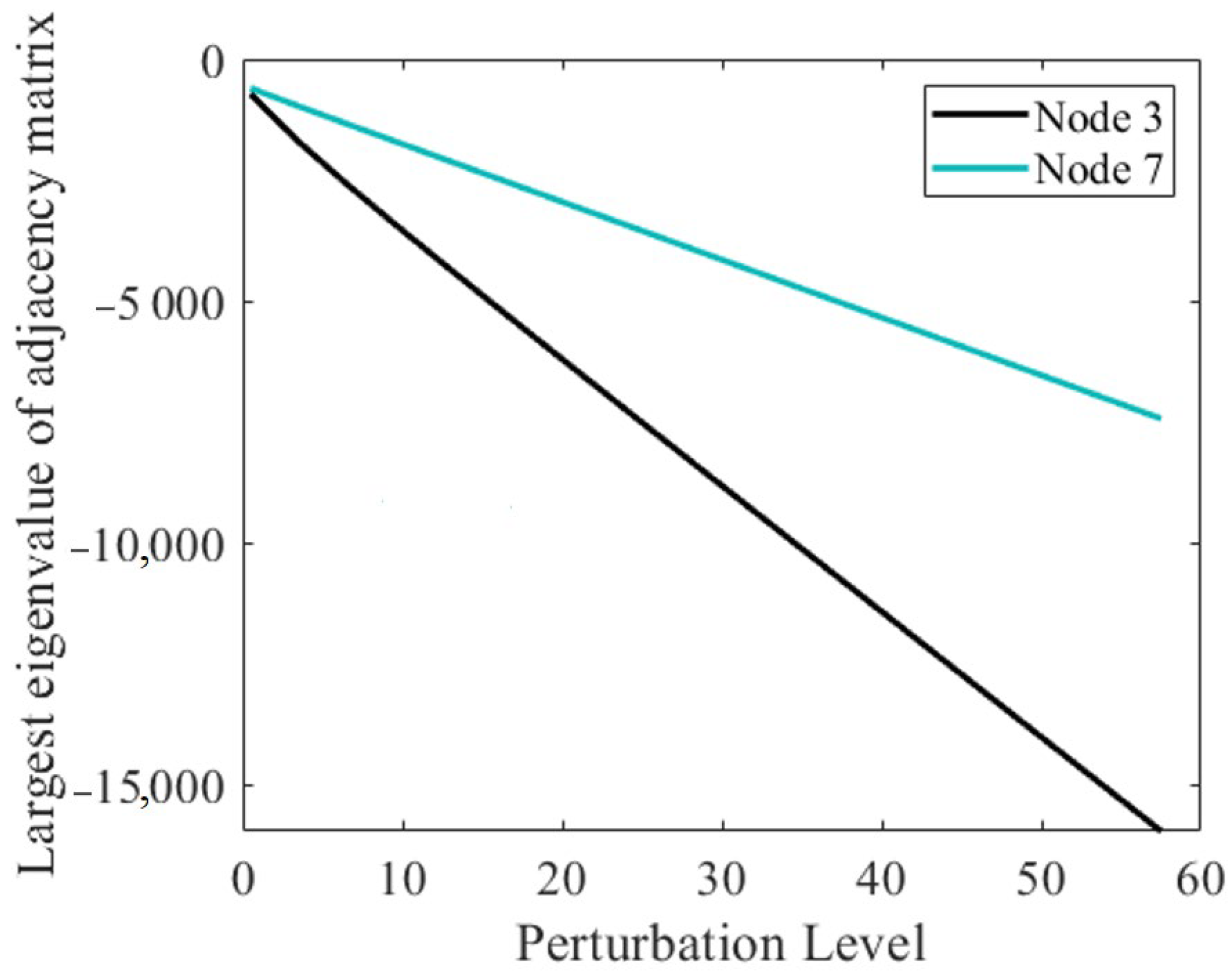
3.2. Spectral Stability Analysis
3.3. Topological Stability Analysis
3.4. Symmetry-Breaking Stability Analysis
4. Discussion and Conclusions
Author Contributions
Funding
Data Availability Statement
Acknowledgments
Conflicts of Interest
Appendix A

References
- Gu, S.; Pasqualetti, F.; Cieslak, M.; Telesford, Q.K.; Yu, A.B.; Kahn, A.E.; Medaglia, J.D.; Vettel, J.M.; Miller, M.B.; Grafton, S.T.; et al. Controllability of structural brain networks. Nat. Commun. 2015, 6, 8414. [Google Scholar] [CrossRef]
- Chen, C.; Zhao, X.; Wang, J.; Li, D.; Guan, Y.; Hong, J. Dynamic graph convolutional network for assembly behavior recognition based on attention mechanism and multi-scale feature fusion. Sci. Rep. 2022, 12, 7394. [Google Scholar] [CrossRef] [PubMed]
- Zhou, P.; Cao, Y.; Li, M.; Ma, Y.; Chen, C.; Gan, X.; Wu, J.; Lv, X. HCCANet: Histopathological image grading of colorectal cancer using CNN based on multichannel fusion attention mechanism. Sci. Rep. 2022, 12, 15103. [Google Scholar] [CrossRef]
- Knyazev, B.; Taylor, G.W.; Amer, M. Understanding attention and generalization in graph neural networks. In Advances in Neural Information Processing Systems (NeurIPS). arXiv 2019, arXiv:1905.02850. [Google Scholar]
- Pirani, M.; Costa, T.; Sundaram, S. Stability of dynamical systems on a graph. In Proceedings of the 53rd IEEE Conference on Decision and Control, Los Angeles, CA, USA, 15–17 December 2014; pp. 613–618. [Google Scholar] [CrossRef]
- Meeks, L.; Rosenberg, D.E. High Influence: Identifying and Ranking Stability, Topological Significance, and Redundancies in Water Resource Networks. J. Water Resour. Plan. Manag. 2017, 143, 04017012. [Google Scholar] [CrossRef]
- Gama, F.; Bruna, J.; Ribeiro, A. Stability Properties of Graph Neural Networks. IEEE Trans. Signal Process. 2020, 68, 5680–5695. [Google Scholar] [CrossRef]
- Yang, F.; Cao, Y.; Xue, Q.; Jin, S.; Li, X.; Zhang, W. Contrastive Embedding Distribution Refinement and Entropy-Aware Attention for 3D Point Cloud Classification. arXiv 2022, arXiv:2201.11388. [Google Scholar]
- Li, A.; Huynh, C.; Fitzgerald, Z.; Cajigas, I.; Brusko, D.; Jagid, J.; Claudio, A.O.; Kanner, A.M.; Hopp, J.; Chen, S.; et al. Neural fragility as an EEG marker of the seizure onset zone. Nat. Neurosci. 2021, 24, 1465–1474, Erratum in Nat. Neurosci. 2022, 25, 530. [Google Scholar] [CrossRef]
- Zhang, Y.; Zhang, Z.; Wei, D.; Deng, Y. Centrality Measure in Weighted Networks Based on an Amoeboid Algorithm. J. Inf. Comput. Sci. 2012, 9, 369–376. [Google Scholar]
- Piraveenan, M.; Prokopenko, M.; Hossain, L. Percolation centrality: Quantifying graph-theoretic impact of nodes during percolation in networks. PLoS ONE 2013, 8, e53095. [Google Scholar] [CrossRef]
- Avena-Koenigsberger, A.; Mišić, B.; Hawkins, R.X.D.; Griffa, A.; Hagmann, P.; Goñi, J.; Sporns, O. Path ensembles and a tradeoff between communication efficiency and resilience in the human connectome. Brain Struct. Funct. 2017, 222, 603–618. [Google Scholar] [CrossRef]
- Kwon, H.; Choi, Y.H.; Lee, J.M. A Physarum Centrality Measure of the Human Brain Network. Sci. Rep. 2019, 9, 5907. [Google Scholar] [CrossRef] [PubMed]
- Kitsak, M.; Gallos, L.; Havlin, S.; Liljeros, F.; Muchnik, L.; Stanley, H.E.; Makse, H.A. Identification of influential spreaders in complex networks. Nat. Phys. 2010, 6, 888–893. [Google Scholar] [CrossRef]
- Sun, Y.; Ma, L.; Zeng, A.; Wang, W.-X. Spreading to localized targets in complex networks. Sci. Rep. 2016, 6, 38865. [Google Scholar] [CrossRef] [PubMed]
- Zhang, C.; Zhou, S.; Miller, J.; Cox, I.J.; Chain, B.M. Optimizing Hybrid Spreading in Metapopulations. Sci. Rep. 2015, 5, 9924. [Google Scholar] [CrossRef] [PubMed]
- Davis, J.T.; Chinazzi, M.; Perra, N.; Mu, K.; Piontti, A.P.Y.; Ajelli, M.; Dean, N.E.; Gioannini, C.; Litvinova, M.; Merler, S.; et al. Cryptic transmission of SARS-CoV-2 and the first COVID-19 wave. Nature 2021, 600, 127–132. [Google Scholar] [CrossRef]
- Le Treut, G.; Huber, G.; Kamb, M.; Kawagoe, K.; McGeever, A.; Miller, J.; Pnini, R.; Veytsman, B.; Yllanes, D. A high-resolution flux-matrix model describes the spread of diseases in a spatial network and the effect of mitigation strategies. Sci. Rep. 2022, 12, 15946. [Google Scholar] [CrossRef]
- Wang, W.; Tang, M.; Yang, H.; Do, Y.; Lai, Y.-C.; Lee, G. Asymmetrically interacting spreading dynamics on complex layered networks. Sci. Rep. 2014, 4, 5097. [Google Scholar] [CrossRef]
- Salnikov, V.; Schaub, M.; Lambiotte, R. Using higher-order Markov models to reveal flow-based communities in networks. Sci. Rep. 2016, 6, 23194. [Google Scholar] [CrossRef]
- Pascual, M. Diffusion-induced chaos in a spatial predator–prey system. Proc. R. Soc. Lond. Ser. B Biol. Sci. 1993, 251, 1–7. [Google Scholar]
- Petrovskii, S.; Li, B.-L.; Malchow, H. Quantification of the Spatial Aspect of Chaotic Dynamics in Biological and Chemical Systems. Bull. Math. Biol. 2003, 65, 425–446. [Google Scholar] [CrossRef] [PubMed]
- Nicolaou, Z.G.; Case, D.J.; Wee, E.B.v.d.; Driscoll, M.M.; Motter, A.E. Heterogeneity-stabilized homogeneous states in driven media. Nat. Commun. 2021, 12, 4486. [Google Scholar] [CrossRef] [PubMed]
- Hammouche, M.; Lutz, P.; Rakotondrabe, M. Robust and Optimal Output-Feedback Control for Interval State-Space Model: Application to a Two-Degrees-of-Freedom Piezoelectric Tube Actuator. Journal of Dynamic Systems, Measurement, and Control. Am. Soc. Mech. Eng. 2018, 141, 021008. [Google Scholar]
- Bloem, P. Transformers from Scratch; VU University: Amsterdam, The Netherlands, 2019. [Google Scholar]
- Velickovic, P.; Cucurull, G.; Casanova, A.; Romero, A.; Lio, P.; Bengio, Y. Graph Attention Networks. arXiv 2018, arXiv:1710.10903. [Google Scholar]
- Chen, B.-S.; Kung, J.-Y. Robust stability of a structured perturbation system in state space models. In Proceedings of the 27th IEEE Conference on Decision and Control, Austin, TX, USA, 7–9 December 1988; Volume 1, pp. 121–122. [Google Scholar] [CrossRef]
- Saberi, M.; Khosrowabadi, R.; Khatibi, A.; Misic, B.; Jafari, G. Topological impact of negative links on the stability of resting-state brain network. Sci. Rep. 2021, 11, 2176. [Google Scholar] [CrossRef]
- Golubitsky, M.; Stewart, I. Symmetry and Bifurcation in Biology; Banff International Research Station (BIRS): Banff, AB, Canada, 2003. [Google Scholar]
- Ruzzenenti, F.; Garlaschelli, D.; Basosi, R. Complex Networks and Symmetry II: Reciprocity and Evolution of World Trade. Symmetry 2010, 2, 1710–1744. [Google Scholar] [CrossRef]
- Goirand, F.; Le Borgne, T.; Lorthois, S. Network-driven anomalous transport is a fundamental component of brain microvascular dysfunction. Nat. Commun. 2021, 12, 7295. [Google Scholar] [CrossRef]
- Broussard, M.A. Diagram of lamellate antenna, 27 March 2016, based on File: Ten-lined June beetle Close-up.jpg. Available online: https://commons.wikimedia.org/wiki/File:Insect-antenna_lamellate.svg (accessed on 28 January 2023).
- Sanchez-Rodriguez, L.M.; Iturria-Medina, Y.; Mouches, P.; Sotero, R.C. Detecting brain network communities: Considering the role of information flow and its different temporal scales. NeuroImage 2021, 225, 117431. [Google Scholar] [CrossRef] [PubMed]
- Fallani Fde, V.; Costa Lda, F.; Rodriguez, F.A.; Astolfi, L.; Vecchiato, G.; Toppi, J.; Borghini, G.; Cincotti, F.; Mattia, D.; Salinari, S.; et al. A graph-theoretical approach in brain functional networks. Possible implications in EEG studies. Nonlinear Biomed. Phys. 2010, 4 (Suppl. 1), S8. [Google Scholar] [CrossRef] [PubMed]
- Rosvall, M.; Esquivel, A.; Lancichinetti, A.; West, J.D.; Lambiotte, R. Memory in network flows and its effects on spreading dynamics and community detection. Nat. Commun. 2014, 5, 4630. [Google Scholar] [CrossRef]
- Zhang, W.-R. Bipolar fuzzy sets and relations: A computational framework for cognitive modeling and multiagent decision analysis. In Proceedings of the 1st International Joint Conference of the North American Fuzzy Information Processing Society Biannual Conference, San Antonio, TX, USA, 18–21 December 1994; pp. 305–309. [Google Scholar]
- Zhang, W.R. NPN fuzzy sets and NPN qualitative algebra: A computational framework for bipolar cognitive modeling and multiagent decision analysis. IEEE Trans. Syst. Man Cybern. Part B Cybern. 1996, 26, 561–575. [Google Scholar] [CrossRef]
- Zhang, W.-R. Equilibrium energy and stability measures for bipolar decision and global regulation. Int. J. Fuzzy Syst. 2003, 5, 114–122. [Google Scholar]
- Zhang, W.-R. Equilibrium relations and bipolar cognitive mapping for online analytical processing with applications in international relations and strategic decision support. IEEE Trans. Syst. Man Cybern. Part B Cybern. 2003, 33, 295–307. [Google Scholar] [CrossRef] [PubMed]
- Zhang, W.-R. Ground-0 Axioms vs. First Principles and Second Law: From the Geometry of Light and Logic of Photon to Mind-Light-Matter Unity-AI&QI. IEEE/CAA J. Autom. Sin. 2021, 8, 534–553. [Google Scholar] [CrossRef]
- Wang, J.; Gao, R.; Zheng, H.; Zhu, H.; Shi, C. SSGCNet: A Sparse Spectra Graph Convolutional Network for Epileptic EEG Signal Classification. arXiv 2022, arXiv:2203.12910. [Google Scholar] [CrossRef] [PubMed]
- Palcu, L.-D.; Supuran, M.; Lemnaru, C.; Dinsoreanu, M.; Potolea, R.; Muresan, R.C. Breaking the interpretability barrier—A method for interpreting deep graph convolutional models. In Proceedings of the International Workshop NFMCP in Conjunction with ECML-PKDD 2019, Wurzburg, Germany, 16 September 2019. [Google Scholar]
- Patil, A.G.; Li, M.; Fisher, M.; Savva, M.; Zhang, H. LayoutGMN: Neural Graph Matching for Structural Layout Similarity. In Proceedings of the 2021 IEEE/CVF Conference on Computer Vision and Pattern Recognition (CVPR) (2020), Seattle, WA, USA, 14–19 June 2020; pp. 11043–11052. [Google Scholar]


| Node Id | Feature Set | ||
|---|---|---|---|
| 0 | 0.5 | −0.1 | 0.3 |
| 1 | 0.2 | 0.1 | 0.7 |
| 2 | −0.5 | 0.7 | −0.1 |
| 3 | −0.1 | −0.6 | 0.4 |
| 4 | 0.3 | −0.5 | −0.2 |
| 5 | 0.1 | −0.1 | −0.4 |
| 6 | 0.3 | 0.8 | −0.1 |
| 7 | 0.1 | −0.2 | 0.2 |
| Node Id | Actual Label | Predicted Output | |
|---|---|---|---|
| Without Perturbation | With Perturbation | ||
| 0 | 0.01 | 0.083 | 0 |
| 1 | 0.20 | 0.189 | 1 |
| 2 | 0.20 | 0.163 | 2 |
| 3 | 0.01 | 0.082 | 3 |
| 4 | 0.01 | 0.083 | 4 |
| 5 | 0.20 | 0.149 | 5 |
| 6 | 0.20 | 0.164 | 6 |
| 7 | 0.01 | 0.083 | 7 |
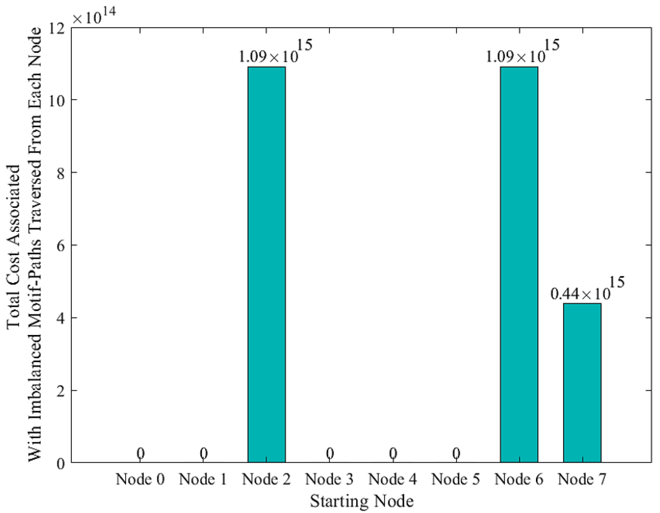
| Node | Three-Node Motif | Four-Node Motif | Five-Node Motif | Six-Node Motif | Total Cost |
|---|---|---|---|---|---|
| 0 | 0.00 | −1.22 × 10⁸ | 0.00 | 0.00 | 0.00 |
| 1 | 0.00 | −2.07 × 10⁹ | −9.32 × 10¹³ | −3.82 × 10¹⁵ | 0.00 |
| 2 | −10,152,500 | −7.41 × 10⁸ | −6.47 × 10¹³ | −2.65 × 10¹⁵ | 1.089 × 10¹⁵ |
| 3 | 0.00 | −5.12 × 10⁸ | −2.33 × 10¹³ | −9.56 × 10¹⁴ | 0.00 |
| 4 | 0.00 | −2.32 × 10⁸ | 0.00 | 0.00 | 0.00 |
| 5 | −29,239,200 | −6.38 × 10⁷ | 0.00 | −3.82 × 10¹⁵ | 0.00 |
| 6 | −10,152,500 | −7.41 × 10⁸ | −6.47 × 10¹³ | −2.65 × 10¹⁵ | 1.089 × 10¹⁵ |
| 7 | −7,309,800 | −5.22 × 10⁸ | −2.33 × 10¹³ | −9.56 × 10¹⁴ | 4.400 × 10¹⁴ |
Disclaimer/Publisher’s Note: The statements, opinions and data contained in all publications are solely those of the individual author(s) and contributor(s) and not of MDPI and/or the editor(s). MDPI and/or the editor(s) disclaim responsibility for any injury to people or property resulting from any ideas, methods, instructions or products referred to in the content. |
© 2023 by the authors. Licensee MDPI, Basel, Switzerland. This article is an open access article distributed under the terms and conditions of the Creative Commons Attribution (CC BY) license (https://creativecommons.org/licenses/by/4.0/).
Share and Cite
Bahador, N.; Lankarany, M. Uncovering the Origins of Instability in Dynamical Systems: How Can the Attention Mechanism Help? Dynamics 2023, 3, 214-233. https://doi.org/10.3390/dynamics3020013
Bahador N, Lankarany M. Uncovering the Origins of Instability in Dynamical Systems: How Can the Attention Mechanism Help? Dynamics. 2023; 3(2):214-233. https://doi.org/10.3390/dynamics3020013
Chicago/Turabian StyleBahador, Nooshin, and Milad Lankarany. 2023. "Uncovering the Origins of Instability in Dynamical Systems: How Can the Attention Mechanism Help?" Dynamics 3, no. 2: 214-233. https://doi.org/10.3390/dynamics3020013