Dark Energy as a Natural Property of Cosmic Polytropes—A Tutorial

Abstract

A conventional approach to the dark energy (DE) concept is reviewed and discussed. According to it, there is absolutely no need for a novel DE component in the universe, provided that its matter–energy content is represented by a perfect fluid whose volume elements perform polytropic flows. When the (thermodynamic) energy of the associated internal motions is taken into account as an additional source of the universal gravitational field, it compensates the DE needed to compromise spatial flatness in an accelerating universe. The unified model which is driven by a polytropic fluid not only interprets the observations associated with universe expansion but successfully confronts all the current issues of cosmological significance, thus arising as a viable alternative to the $\Lambda$CDM model.

1. Introduction

According to a considerable amount of observational data accumulated in the last 25 years, it became evident that a uniformly distributed energy component, so-called DE, is present in the universe (see, e.g., [1,2]). First, it was the high-precision distance measurements, performed with the aid of distant supernova type Ia (SNe Ia) events, which revealed that, in a dust universe (i.e., under the assumption that the constituents of the universe matter content do not interact with each other, so that their world lines remain eternally parallel), these standard candles look fainter (i.e., they are located farther) than what was theoretically predicted [3,4,5,6,7,8,9,10,11,12,13,14,15,16,17,18,19,20,21,22,23,24,25,26,27,28,29,30,31]. To interpret this result, Perlmutter et al. [2] and Riess et al. [9], following Carroll et al. [32], admitted that the long sought cosmological constant, $\Lambda$, differs from zero; hence, apart from matter, the universe also contains a uniformly distributed amount of energy [33]. The need for an energy component that does not cluster at any scale was subsequently verified by observations of galaxy clusters [34], the integrated Sachs–Wolfe effect [35], baryon acoustic oscillations (BAOs) [36,37], weak gravitational lensing [38,39], and the Lyman-$\alpha$ forest [40]. If this energy component is due to the cosmological constant, it would necessarily introduce a repulsive gravitational force [41]; hence, the unexpected dimming of the SNe Ia standard candles was accordingly attributed to a recent acceleration of universe expansion (see, e.g., [42,43,44]).

At the same time, high precision cosmic microwave background (CMB) observations suggested that our universe is, in fact, a spatially flat Robertson–Walker (RW) cosmological model [45,46,47,48,49,50,51,52,53,54,55,56]. This means that the overall energy density, $\epsilon$, of the universe matter–energy content, in units of the critical energy density, ${\epsilon }_c={\rho }_c{c}^2$ (the equivalent to the critical rest-mass density, ${\rho }_c=\frac{3H_0^2}{8\pi G}$, where $H_0$ is the Hubble parameter at the present epoch, G is Newton’s gravitational constant, and c is the velocity of light), must be equal to unity, $\Omega =\frac{\epsilon }{{\epsilon }_c}=1$, i.e., much larger than the measured value of the mass-density parameter, ${\Omega }_M=\frac{\rho }{{\rho }_c}=0.302\pm 0.006$, where $\rho$ is the rest-mass density [57]. Therefore, an extra amount of energy was also needed, to justify spatial flatness.

Quantum vacuum could serve as such an energy basin, attributing an effective cosmological constant to the universe, which would justify both spatial flatness and accelerated expansion [33,41,58]. Unfortunately, vacuum energy is ${10}^{123}$ times larger than the associated measured quantity in curved spacetime [58]. Clearly, an approach other than the cosmological constant (namely, the DE) was needed to incorporate spatial flatness in an accelerating universe; hence, (too) many models were proposed. An (only) indicative list would involve quintessence [59], k-essence [60], and other (more exotic) scalar fields [61], tachyons [62], brane cosmology [63,64], scalar–tensor gravity [65], $f\left(R\right)$-theory [66,67], holographic principle [68,69,70], Chaplygin gas [71,72,73,74], Cardassian cosmology [75,76,77], multidimensional cosmology [78,79,80,81], mass-varying neutrinos [82,83], cosmological principle deviations [84,85,86,87], and many other models (see, e.g., [88]), not to mention the associated cosmographic results [89,90,91,92,93,94,95,96,97,98,99,100,101,102,103,104,105,106,107,108]. In an effort to illuminate darkness, we point out that, long before the necessity of DE’s invention, another dark component was (and still is) present in the composition of the universe matter content, the long sought dark matter (DM).

Today, there is absolutely no doubt as regards the existence of a non-luminous mass component in the universe. The associated observational data involve high-precision measurements of the flattened galactic rotation curves [109,110], weak gravitational lensing [111], and modulation of the strong lensing effects due to massive elliptical galaxies [112]. On a galactic scale, it was found that their dark haloes extend almost half the distance to the neighboring cosmic structures [113,114], while, at even larger scales, the total mass of galaxy clusters is proved to be tenfold as compared to their baryonic mass [115,116,117]. The same is also true at the universe level, as it is inferred from the combination of CMB observations [53] and light chemicals’ abundances [118]. In view of all the above, it is now well established that $85\%$ of the universe mass content is non-luminous and, most probably, non-baryonic [119].

The precise nature of DM constituents is still unknown. There are many candidates, from ordinary stellar-size black holes, to Bose–Einstein condensates and ultralight axions [120]. Another interesting candidate is the weakly interacting massive particles (WIMPs) [121,122,123], which can be relevant to a potential detection of DM, because they annihilate through standard-model channels [124,125]. However, regarding WIMPs, only weak-scale physics is involved and, therefore, we argued that, practically, they do not interact with each other. Nevertheless, a few years ago, particle detectors [126,127] and the Wilkinson Microwave Anisotropy Probe (WMAP) [128] have revealed an unexpected excess of cosmic positrons, which might be due to WIMP collisions (see, e.g., [129,130,131,132,133,134,135,136,137,138,139]). In other words, WIMPs can be slightly collisional [140,141,142,143,144].

A cosmological model of self-interacting matter content could in fact unify DM and DE between them [145,146,147,148,149,150,151,152,153,154,155,156,157,158]). In this framework, Kleidis and Spyrou [159,160,161,162,163] admitted that the potential collisions of WIMPs maintain a tight coupling between them and their kinetic energy is re-distributed. On this assumption, DM itself acquires fluid-like properties and, hence, universe evolution is now driven by a fluid whose volume elements perform hydrodynamic flows (and not by dust). In our defense, the same assumption has also been used in modeling dark galactic haloes, significantly improving the corresponding velocity dispersion profiles [164,165,166,167,168,169,170]. If this is the case, the thermodynamic energy of the DM fluid internal motions should also be considered as a component of the universe matter energy content that drives cosmic expansion. We cannot help but wonder whether it could also compensate for the extra DE needed to compromise spatial flatness or not.

This review article is organized as follows: In Section 2, we consider a spatially flat cosmological model whose evolution is driven by a (perfect) fluid of DM, the volume elements of which perform polytropic flows [160,161,162,163]. Accordingly, an extra energy amount—the energy of internal motions—arises naturally and compensates the extra DE needed to compromise spatial flatness. Such a cosmological model involves a free parameter, the associated polytropic exponent, $\Gamma$. In the case where $\Gamma <1$ the cosmic pressure becomes negative and the universe accelerates its expansion below a particular value of the cosmological redshift parameter, z, the so-called transition redshift,$z_{tr}$. In Section 3, we demonstrate that the polytropic DM model so assumed can confront all the major issues of cosmological significance, since, in the constant pressure (i.e., $\Gamma =0$) limit, it fully reproduces all the predictions and the associated observational results concerning the infernous$\Lambda$CDM model [160,161,162]. Finally, we conclude in Section 4.

2. Polytropic Flows in a Cosmological DM Fluid

CMB has been proved a most valuable tool for reliable cosmological observations (see, e.g., [45,46,47,48,49,50,51,52,53,54,55,56]). At the present epoch, data arriving from various CMB probes strongly suggest that the universe can be described by a spatially flat RW model, i.e.,

$$d{s}^2=c^{2}d{t}^2-S^2\left(t\right)\left(d{x}^2+d{y}^2+d{z}^2\right),$$

(1)

where $S\left(t\right)$ is the scale factor as a function of cosmic time, t. The evolution of the cosmological model given by Equation (1) depends on the exact form and the properties of its matter–energy content.

According to Kleidis and Spyrou [159,160,161,162,163], in a universe filled with interactive DM there is absolutely no need for an extra DE component. Indeed, provided that the collisions of the DM constituents are frequent enough, they can maintain a tight coupling between them so that their kinetic energy is re-distributed. In this case, the universe matter content acquires thermodynamic properties and the curved spacetime evolution is driven by a perfect (DM) fluid instead of pressureless dust [159]. Due to the cosmological principle, this fluid is practically homogeneous and isotropic at large scale and, therefore, its pressure, p, obeys an EoS of the form $p=f\left(\rho \right)$ [160]. Now, the fundamental units of the universe matter content are the volume elements of this (DM) fluid, i.e., closed thermodynamical systems with conserved number of particles [171]. Their motion in the interior of the cosmic fluid under consideration is determined by the conservation law

$$T_{;\nu }^{\mu \nu }=0,$$

(2)

where Greek indices refer to four-dimensional spacetime, Latin indices refer to three-dimensional space, the semicolon denotes covariant derivative, and $T^{\mu \nu }$ is the energy-momentum tensor of the source that drives universe evolution. In the particular case of a perfect fluid, $T^{\mu \nu }$ reads

$$T^{\mu \nu }=(\epsilon +p)u^{\mu }{u}^{\nu }-p{g}^{\mu \nu },$$

(3)

where $u^{\mu }$ is the four-velocity $\left(u_{\mu }{u}^{\mu }=1\right)$, $g^{\mu \nu }$ is the universe metric tensor, and $\epsilon$ is the total energy density of the fluid, which, now, is decomposed to

$$\epsilon =ϵ(\rho ,T)+\rho U\left(T\right)$$

(4)

(see, e.g., [172], pp. 81–84 and 90–94). In Equation (4), T is the absolute temperature, $U\left(T\right)$ is the energy of this fluid’s internal motions, and $ϵ(\rho ,T)$ represents all forms of energy besides that of internal motions. In view of Equation (4), Equation (2) represent the hydrodynamic flows of volume elements in the interior of a perfect-fluid source as they are traced by an observer comoving with cosmic expansion in a maximally symmetric cosmological model (see, e.g., [173], p. 91). The evolution of such a model (see, e.g., [173] pp. 61, 62) can be determined by the Friedmann equation of the classical Friedmann–Robertson–Walker (FRW) cosmology

$$H^2=\frac{8\pi G}{3c^2}\epsilon ,$$

(5)

where

$$H=\frac{\dot{S}}{S}$$

(6)

is the Hubble parameter in terms of $S\left(t\right)$ and the dot denotes differentiation with respect to cosmic time. To solve Equation (5), first we need to determine $\epsilon$, in other words $ϵ$ and U. To do so, we use the first law of thermodynamics in curved spacetime,

$$dU+pd\left(\frac{1}{\rho }\right)=\mathcal{C}dT$$

(7)

(see, e.g., [172], p. 83), where $\mathcal{C}$ is the specific heat of the cosmic fluid, in connection with the zeroth component of Equation (2), i.e., the continuity Equation

$$\dot{\epsilon }+3\frac{\dot{S}}{S}(\epsilon +p)=0.$$

(8)

Finally, we need to decide on the form of the function $p=f\left(\rho \right)$. Accordingly, we admit that the volume elements of the universe matter content perform polytropic flows [160,161,162,163].

Polytropic process is a reversible thermodynamic process in which the specific heat of a closed system evolves in a well-defined manner (see, e.g., [174], p. 2). For $\mathcal{C}=constant$, the system possesses only one independent state variable, the rest-mass density, and the EoS for a perfect fluid, $p\propto \rho T$ , results in

$$\begin{array}{ccc}\hfill p& =& p_0{\left(\frac{\rho }{{\rho }_0}\right)}^{\Gamma }\hfill \end{array}$$

(9)

$$\begin{array}{ccc}\hfill T& =& T_0{\left(\frac{\rho }{{\rho }_0}\right)}^{\Gamma -1}\hfill \end{array}$$

(10)

(see, e.g., [160]), where $p_0$, ${\rho }_0$, and $T_0$ denote the present-time values of pressure, rest-mass density, and temperature, respectively, and $\Gamma$ is the polytropic exponent. In such a model, Equation (7) yields

$$U=U_0{\left(\frac{\rho }{{\rho }_0}\right)}^{\Gamma -1},$$

(11)

where

$$U_0=\mathcal{C}{T}_0+\frac{1}{\Gamma -1}\frac{p_0}{{\rho }_0}$$

(12)

is the present-time value of the cosmic fluid internal energy. In view of Equations (4) and (11), Equation (8) is written in the form

$$\Gamma U_0\left(\dot{\rho }+3\frac{\dot{S}}{S}\rho \right)+\dot{ϵ}+3\frac{\dot{S}}{S}ϵ-3(\Gamma -1){\rho }_0\mathcal{C}{T}_0\frac{\dot{S}}{S}{\left(\frac{\rho }{{\rho }_0}\right)}^{\Gamma }=0.$$

(13)

Since the total number of particles in a closed system (volume element) is conserved, we furthermore have

$$\dot{\rho }+3\frac{\dot{S}}{S}\rho =0\Rightarrow \rho ={\rho }_0{\left(\frac{S_0}{S}\right)}^3$$

(14)

and, therefore, Equation (13) results in

$$ϵ={\rho }_0{c}^2{\left(\frac{S_0}{S}\right)}^3-{\rho }_0\mathcal{C}{T}_0{\left(\frac{S_0}{S}\right)}^{3\Gamma }.$$

(15)

By virtue of Equations (11)–(15), the total energy density (4) of the polytropic DM model under consideration is written in the form

$$\epsilon ={\rho }_0{c}^2{\left(\frac{S_0}{S}\right)}^3+\frac{p_0}{\Gamma -1}{\left(\frac{S_0}{S}\right)}^{3\Gamma }=\rho c^2+\frac{1}{\Gamma -1}p$$

(16)

and the Friedmann Equation (5) results in

$${\left(\frac{H}{H_0}\right)}^2={\Omega }_M{\left(\frac{S_0}{S}\right)}^3\left[1+\frac{1}{\Gamma -1}\frac{p_0}{{\rho }_0{c}^2}{\left(\frac{S_0}{S}\right)}^{3(\Gamma -1)}\right].$$

(17)

Extrapolation of Equation (17) to the present epoch yields the corresponding value of the polytropic DM fluid pressure, i.e.,

$$p_0={\rho }_0{c}^2(\Gamma -1)\frac{1-{\Omega }_M}{{\Omega }_M}.$$

(18)

In view of Equation (18), for $\Gamma <1$, the pressure (9) is negative and so might be the quantity $\epsilon +3p$, as well, something that would lead to $\ddot{S}>0$ (see, e.g., [43]). In other words, for $\Gamma <1$, the polytropic DM model under consideration can accelerate its expansion. At the same time, Equation (16) reads

$$\epsilon ={\rho }_c{c}^2\left[{\Omega }_M{\left(\frac{S_0}{S}\right)}^3+(1-{\Omega }_M){\left(\frac{S_0}{S}\right)}^{3\Gamma }\right],$$

(19)

the extrapolation of which to the present epoch suggests that the total energy density parameter of the polytropic DM model under consideration is exactly unity, i.e.,

$${\Omega }_0=\frac{{\epsilon }_0}{{\epsilon }_c}=\frac{{\rho }_c{c}^2}{{\rho }_c{c}^2}\left[{\Omega }_M+(1-{\Omega }_M)\right]=1.$$

(20)

We see that the polytropic DM model with $\Gamma <1$ might be an excellent conventional solution to the DE issue, by comprising both spatial flatness $({\Omega }_0=1)$ and accelerated expansion $(\epsilon +3p<0)$ of the universe in a unique theoretical framework.

3. Predictions and Outcomes of the Polytropic DM Model

In this Section, we explore the properties of a polytropic DM model with $\Gamma <1$, in association with all the major issues of cosmological significance. To do so, unless otherwise stated, in what follows we admit that ${\Omega }_M=0.274$, as suggested by the nine years WMAP survey [54]. This value differs from the corresponding Planck result, ${\Omega }_M=0.308$ [55,56], and/or the most recent observational one, ${\Omega }_M=0.302$, of the Dark Energy Survey (DES) consortium [57], while resting quite far also from its Pantheon Compilation counterpart, ${\Omega }_M=0.306$ [30]. It is evident that the exact value of ${\Omega }_M$, as also of many other parameters of cosmological significance (see, e.g., [175]), is still a matter of debate.

3.1. The Accelerated Expansion of the Universe

Upon consideration of Equation (18), Equation (17) is written in the form

$${\left(\frac{H}{H_0}\right)}^2={\left(\frac{S_0}{S}\right)}^3\left[{\Omega }_M+(1-{\Omega }_M){\left(\frac{S}{S_0}\right)}^{3(1-\Gamma )}\right]$$

(21)

or, in terms of the cosmic scale factor, in the more convenient form

$${\left[\frac{d}{dt}{\left(\frac{S}{S_0}\right)}^{3/2}\right]}^2=\frac{1}{t_{EdS}^2}\left\{{\Omega }_M+(1-{\Omega }_M){\left[{\left(\frac{S}{S_0}\right)}^{3/2}\right]}^{2(1-\Gamma )}\right\},$$

(22)

where $t_{EdS}=\frac{2}{3H_0}$ is the age of the universe in the Einstein–de Sitter (EdS) model. Equation (22) can be solved in terms of hypergeometric functions, as follows

$${\left(\frac{S}{S_0}\right)}^{\frac{3}{2}}{}_2{F}_1\left(\frac{1}{2(1-\Gamma )},\frac{1}{2};\frac{3-2\Gamma }{2(1-\Gamma )};-\left(\frac{1-{\Omega }_M}{{\Omega }_M}\right){\left[\frac{S}{S_0}\right]}^{3(1-\Gamma )}\right)=\sqrt{{\Omega }_M}\left(\frac{t}{t_{EdS}}\right)$$

(23)

(cf. [176], pp. 1005–1008). For $\Gamma <1$, the resulting hypergeometric series converges absolutely within the circle of (unit) radius $\left|\frac{S}{S_0}\right|\le 1$ (cf. [177], p. 556). There are two limiting cases of Equation (23) of particular interest: (i) For ${\Omega }_M=1$, it yields $S=S_0{\left(\frac{t}{t_{EdS}}\right)}^{2/3}$, i.e., the scale factor of the EdS model. (ii) For $\Gamma =0$ (i.e., in the $\Lambda$CDM-like limit), Equation (23) is written in the form

$${\left(\frac{S}{S_0}\right)}^{\frac{3}{2}}{}_2{F}_1\left(\frac{1}{2},\frac{1}{2};\frac{3}{2};-\left(\frac{1-{\Omega }_M}{{\Omega }_M}\right){\left[\frac{S}{S_0}\right]}^3\right)=\sqrt{{\Omega }_M}\left(\frac{t}{t_{EdS}}\right),$$

(24)

which, upon consideration of the identity

$${}_2{F}_1\left(\frac{1}{2},\frac{1}{2};\frac{3}{2};-x^2\right)=\frac{1}{x}{sinh}^{-1}\left(x\right)$$

(25)

(cf. [176], Equation (9.121.28), p. 1007, [177], Equation (15.1.7), p. 556), where in our case, $x=\sqrt{\left(\frac{1-{\Omega }_M}{{\Omega }_M}\right){\left[\frac{S}{S_0}\right]}^3}$, results in

$$S\left(t\right)=S_0{\left(\frac{{\Omega }_M}{1-{\Omega }_M}\right)}^{1/3}{sinh}^{2/3}\left(\sqrt{1-{\Omega }_M}\frac{t}{t_{EdS}}\right).$$

(26)

For $1-{\Omega }_M={\Omega }_{\Lambda }$, Equation (26) represents the scale factor of the $\Lambda$CDM model (cf. Equation (5) of [178]), as it should. On the other hand, at the present epoch, i.e., when $t=t_0$ and $S=S_0$, Equation (23) reads

$$\frac{t_0}{t_{EdS}}=\frac{1}{\sqrt{{\Omega }_M}}{}_2{F}_1\left(\frac{1}{2(1-\Gamma )},\frac{1}{2};1+\frac{1}{2(1-\Gamma )};-\frac{1-{\Omega }_M}{{\Omega }_M}\right).$$

(27)

With the aid of Equation (27) we can eliminate $t_{EdS}$ from Equation (23), to obtain the scale factor of the polytropic DM model (in units of $S_0$) as a function of cosmic time (in units of $t_0$), i.e.,

$${\left(\frac{S}{S_0}\right)}^{3/2}\frac{{}_2{F}_1\left(\frac{1}{2(1-\Gamma )},\frac{1}{2};\frac{3-2\Gamma }{2(1-\Gamma )};-\left(\frac{1-{\Omega }_M}{{\Omega }_M}\right){\left[\frac{S}{S_0}\right]}^{3(1-\Gamma )}\right)}{{}_2{F}_1\left(\frac{1}{2(1-\Gamma )},\frac{1}{2};\frac{3-2\Gamma }{2(1-\Gamma )};-\frac{1-{\Omega }_M}{{\Omega }_M}\right)}=\frac{t}{t_0}.$$

(28)

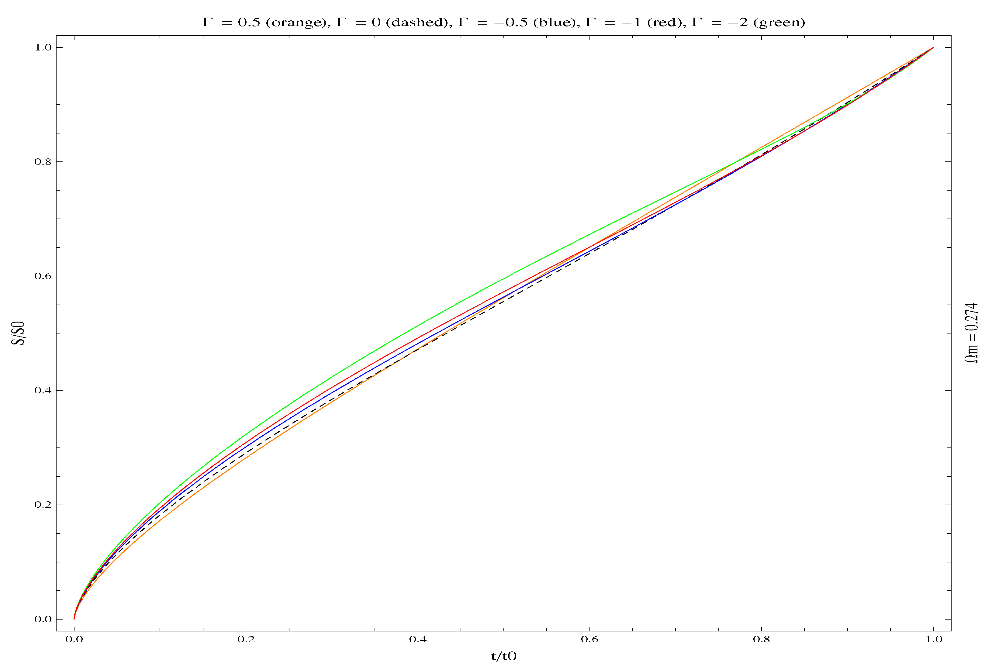
The evolution of $S\left(t\right)$ (in units of $S_0$) parameterized by $\Gamma <1$, is given in Figure 1. We observe that, in all cases, there is a value of $t<t_0$ (somewhere around $t\simeq 0.75t_0$), above which the function $S\left(t\right)$ becomes concave, i.e., $\ddot{S}>0$. This is a very important result, indicating that the polytropic DM model with $\Gamma <1$ definitely transits from deceleration to acceleration at a certain time, (quite) close to the present epoch, $t_0$.

3.2. The Age of the Universe

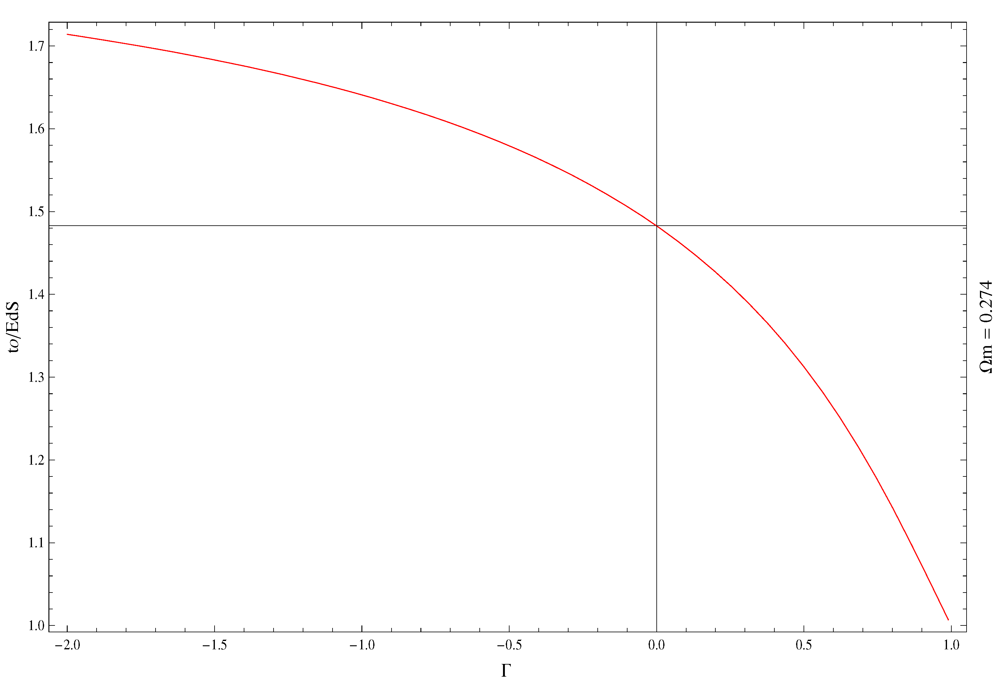
By construction, Equation (27) represents the age, $t_0$, of the polytropic DM universe in units of $t_{EdS}$. The behavior of $t_0$, as a function of the polytropic exponent $\Gamma <1$, is presented in Figure 2. In the $\Lambda$CDM-like $(\Gamma =0)$ limit, Equation (27) yields

$$t_0=t_{EdS}\frac{1}{\sqrt{1-{\Omega }_M}}{sinh}^{-1}\sqrt{\frac{1-{\Omega }_M}{{\Omega }_M}}.$$

(29)

For ${\Omega }_M=0.274$, Equation (29) results in $t_0=1.483t_{EdS}$, which, adopting that $H_0\simeq 67.5$ km/s/Mpc (see, e.g., [54,57]), yields $t_0=13.79Gys$. This theoretically predicted value of $t_0$ is in excellent agreement with the corresponding observational result [54,55,56,57] for the age of the $\Lambda$CDM universe. In fact, from Figure 2 we see that, for every $\Gamma <1$, the age of the polytropic DM model is always larger than that of its EdS counterpart; in other words, the polytropic DM model so assumed no longer suffers from what is referred to as the age problem.

3.3. Transition to Acceleration

In the polytropic DM model under consideration the Hubble parameter (21) in terms of the cosmological redshift, $1+z=\frac{S_0}{S}$, is written in the form

$$H=H_0{(1+z)}^{\frac{3}{2}}{\left[{\Omega }_M+\frac{1-{\Omega }_M}{{(1+z)}^{3(1-\Gamma )}}\right]}^{1/2}.$$

(30)

In view of Equation (30), the deceleration parameter

$$q\left(z\right)=\frac{dH/dz}{H\left(z\right)}(1+z)-1$$

(31)

reads

$$q\left(z\right)=\frac{1}{2}\left[1-\frac{3(1-\Gamma )(1-{\Omega }_M)}{{\Omega }_M{(1+z)}^{3(1-\Gamma )}+(1-{\Omega }_M)}\right].$$

(32)

For $z=0$ (i.e., at the present epoch), we obtain

$$q_0=\frac{1}{2}\left[1-3(1-\Gamma )(1-{\Omega }_M)\right],$$

(33)

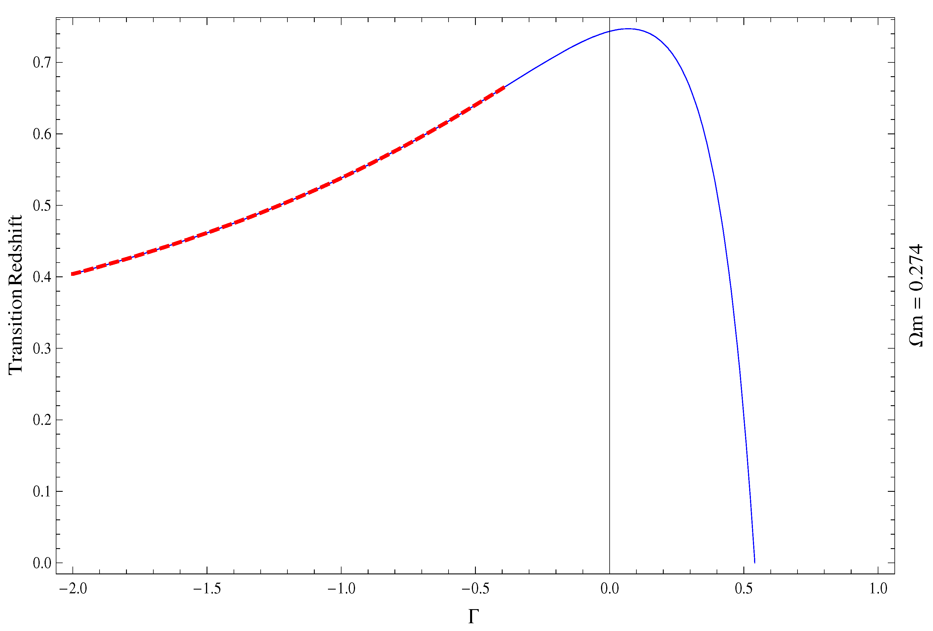
which, in the $\Lambda$CDM-like (i.e., $\Gamma =0)$ limit, yields $q_0=-0.54$. This result lies well within the associated observationally determined range of $q_0$, i.e., $q_0=-0.{53}_{-0.13}^{+0.15}$ [179], and, in fact, reproduces the corresponding (i.e., theoretically derived) $\Lambda$CDM result, that is, $q_0=-0.55\pm 0.01$ [180]. However, what is more important is that the condition $q\left(z\right)\le 0$ reveals a particular value of z, the so-called transition redshift,

$$z_{tr}={\left[(2-3\Gamma )\frac{1-{\Omega }_M}{{\Omega }_M}\right]}^{\frac{1}{3(1-\Gamma )}}-1,$$

(34)

below which $q\left(z\right)$ becomes negative, i.e., the universe accelerates its expansion. In the $\Lambda$CDM-like $(\Gamma =0)$ limit, Equation (34) yields $z_{tr}=0.744$, which (i) lies well within range of the corresponding $\Lambda$CDM result, namely, $z_{tr}=0.752\pm 0.041$ [29] and (ii) actually reproduces the associated result of Muccino et al. [181], i.e., $z_{tr}=0.{739}_{-0.089}^{+0.065}$, obtained by applying a model-independent method to a number of SNeIa, BAOs, and GRB data. Furthermore, by virtue of Equation (34), the condition $z_{tr}\ge 0$ imposes a more stringent constraint on the potential values of $\Gamma$, namely,

$$\Gamma \le \frac{1}{3}\left[2-\frac{{\Omega }_M}{1-{\Omega }_M}\right].$$

(35)

For ${\Omega }_M=0.274$, Equation (35) yields $\Gamma \le 0.541$. Apparently, the polytropic DM model with $\Gamma \le 0.541$ accelerates its expansion at cosmological redshifts lower than a transition value, without the need of any novel DE component. The behavior of $z_{tr}$, as a function of the parameter $\Gamma \le 0.541$, is presented in Figure 3.

3.4. The Total EoS Parameter

In the $\Lambda$CDM-like $(\Gamma =0)$ limit, our model actually reproduces the behavior of the (so-called) total EoS parameter,

$$w_{tot}\equiv \frac{p}{\epsilon },$$

(36)

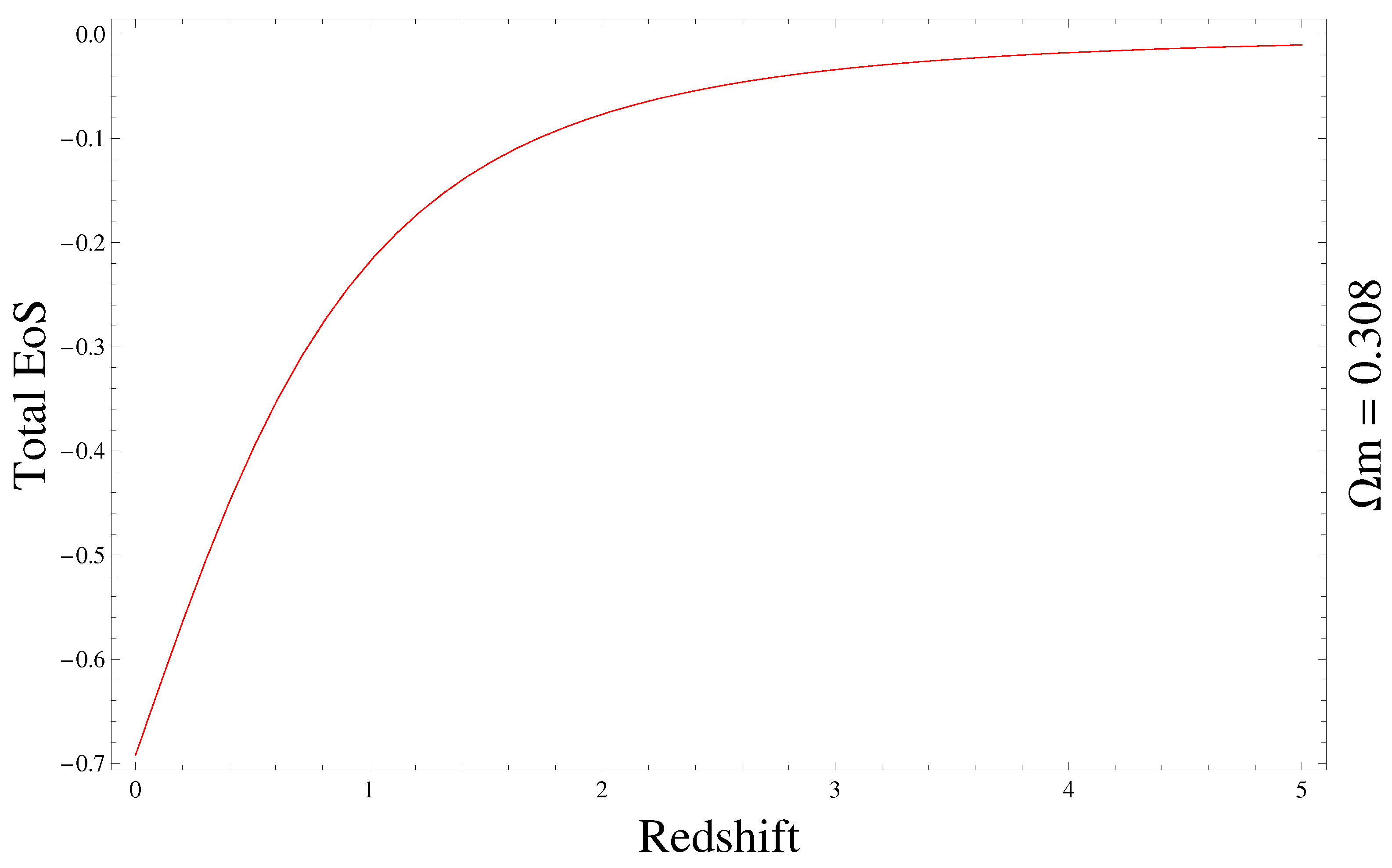
as a function of z [88]. For $\Gamma =0$, upon consideration of Equations (14), (16), and (18), Equation (36) yields

$$w_{tot}\equiv \frac{p}{\epsilon }=-\frac{1-{\Omega }_M}{1-{\Omega }_M+{\Omega }_M{(1+z)}^3},$$

(37)

the behavior of which, in terms of the cosmological redshift parameter, is depicted in Figure 4. Today, i.e., for $z=0$, we have $w_{tot}=-\left(1-{\Omega }_M\right)=-{\Omega }_{\Lambda }$, in complete correspondence to the associated $\Lambda$CDM result,

$$w_{tot}=\frac{p_{tot}}{{\rho }_{tot}}=\frac{p_{\Lambda }}{{\rho }_M+{\rho }_{\Lambda }}=\frac{-{\rho }_{\Lambda }}{{\rho }_M+{\rho }_{\Lambda }}=\frac{-{\Omega }_{\Lambda }}{{\Omega }_M+{\Omega }_{\Lambda }}=-{\Omega }_{\Lambda }$$

(38)

(in connection, see, e.g., [88]).

3.5. The Range of Values of the Polytropic Exponent

The isentropic velocity of sound is defined as

$$c_s^2=c^2{\left(\frac{\partial p}{\partial \epsilon }\right)}_{\mathcal{S}}$$

(39)

(see, e.g., [182] p. 52), where ${\left(\frac{\partial p}{\partial \epsilon }\right)}_{\mathcal{S}}\le 1$, in order to avoid violation of causality [183]. In the polytropic DM model, the total energy density of the universe matter–energy content is related to pressure by Equation (16), whose partial differentiation yields the associated velocity of sound as a function of z,

$${\left(\frac{c_s}{c}\right)}^2=-\frac{\Gamma (1-\Gamma )\frac{1-{\Omega }_M}{{\Omega }_M}}{{(1+z)}^{3(1-\Gamma )}+\Gamma \frac{1-{\Omega }_M}{{\Omega }_M}}.$$

(40)

Now, the condition for a positive (or zero) velocity-of-sound square imposes a major constraint on $\Gamma$, i.e.,

$${\left(\frac{c_s}{c}\right)}^2\ge 0\iff \Gamma \le 0,$$

(41)

while, admitting that, today, DM is cold, i.e., at $z=0$,

$${\left(\frac{c_s}{c}\right)}^2<\frac{1}{3},$$

(42)

we obtain

$$\Gamma >-\frac{2}{3}\left[\sqrt{1+\frac{3}{4}\frac{{\Omega }_M}{1-{\Omega }_M}}-1\right]=-0.1.$$

(43)

Equations (41) and (43) significantly narrow the potential range of values of the polytropic exponent, which, from now on, rests in

$$-0.1<\Gamma \le 0.$$

(44)

Hence, in the polytropic DM model under consideration, the associated polytropic exponent, if not zero, is definitely negative and very close to zero. Notice that, in view of Equation (44), Equation (9) is in excellent agreement with the associated result for a generalized Chaplygin gas, $p\sim -{\rho }^{\alpha }$, arising from the combination of X-ray and SNe Ia measurements with data from Fanaroff–Riley type IIb radio-galaxies, namely, $\alpha =-0.{09}_{-0.33}^{+0.54}$ [184].

3.6. The Jerk Parameter

A dimensionless third (time-)derivative of the scale factor, $S\left(t\right)$, the so-called jerk parameter,

$$j\left(S\right)=\frac{1}{S{H}^3}\frac{d^{3}S}{d{t}^3}$$

(45)

(see, e.g., [185,186]), can be used to demonstrate the departure of the polytropic DM model under consideration from its $\Lambda$CDM counterpart. The reason is that, for the $\Lambda$CDM model $j=1$, for every z. Hence, any deviation of j from unity enables us to constrain the departure of the model so assumed from the $\Lambda$CDM model in an effective manner [186].

In terms of the deceleration parameter, j is written in the form

$$j\left(q\right)=q(2q+1)+(1+z)\frac{dq}{dz}$$

(46)

(see, e.g., [187]), which, in the polytropic DM model, i.e., upon consideration of Equation (32), yields

$$j\left(z\right)=1-\frac{9}{2}\Gamma \frac{(1-\Gamma )}{1+\frac{{\Omega }_M}{1-{\Omega }_M}{(1+z)}^{3(1-\Gamma )}}.$$

(47)

Notice that, for $\Gamma =0$, $j=1$; hence, once again, the $\Gamma =0$ limit of the polytropic DM model under consideration does reproduce the $\Lambda$CDM model. Now, by virtue of Equation (41), the jerk parameter (47) reads

$$j\left(z\right)=1+\frac{9}{2}|\Gamma |\frac{(1+|\Gamma \left|\right)}{1+\frac{{\Omega }_M}{1-{\Omega }_M}{(1+z)}^{3(1+|\Gamma \left|\right)}},$$

(48)

i.e., it is always positive. This is a very important result, since it guarantees that, at $z_{tr}$, a (phase) transition of the universe expansion from deceleration to acceleration actually takes place (in connection, see [186,188]).

Two values of $j\left(z\right)$ are of particular interest: (i) its present-time $(z=0)$ value, given by

$$j_0\equiv j(z=0)=1+\frac{9}{2}|\Gamma |(1+|\Gamma |),$$

(49)

which, in view of Equation (44), results in

$$1\le j_0<1.495,$$

(50)

clearly discriminating the $\Gamma \ne 0$ polytropic DM model from its $\Lambda$CDM counterpart; and (ii) the value of the jerk parameter at transition $(z=z_{tr})$, which, upon consideration of Equation (34), it is given by

$$j_{tr}\equiv j\left(z_{tr}\right)=1+\frac{3}{2}|\Gamma |.$$

(51)

In this case, we return (once again) to Muccino et al. [181] to use the corresponding model-independent constraints on $j_{tr}$, in order to estimate the value of the polytropic index, $|\Gamma |$, in a model-independent way. Accordingly, adopting the best-fit value $j_{tr}=1.028$ of [181], obtained by means of the DHE method (see [188]), Equation (51) yields

$$|\Gamma |=0.02,$$

while, adopting the corresponding DDPE value [188], $j_{tr}=1.041$, Equation (51) results in

$$|\Gamma |=0.03.$$

Both values not only favor a $\Gamma \ne 0$ polytropic DM model but also are well within range of Equation (44), i.e., once again, compatibility of the polytropic DM model with observation is well established.

In view of [186], we cannot help but wondering whether the polytropic DM model with a jerk parameter given by Equation (48) is also compatible with the Union 2.1 Compilation of the SNe Ia data or not.

3.7. The Hubble Diagram of the SNe Ia Data

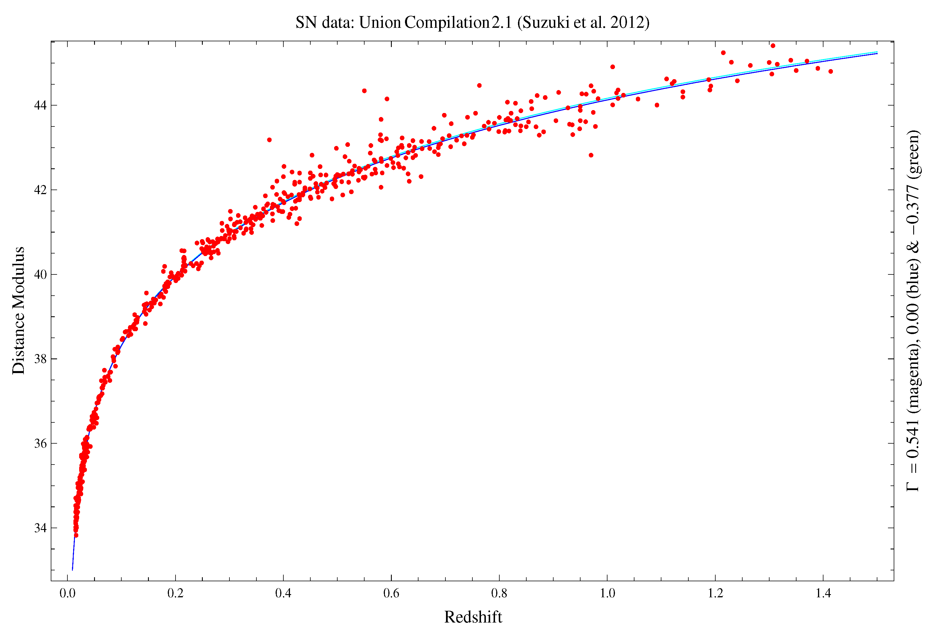
Today, (too) many samples of SNe Ia data are used to scrutinize the viability of the DE models proposed. One of the most extended is the Union 2.1 Compilation [29], consisting of 580 SNe Ia events, being inferior only to the (so-called) Pantheon Compilation [30]. We shall use the former sample to demonstrate compatibilty of the theoretically derived (in the context of the polytropic DM model) formula for the distance modulus,

$$\mu \left(z\right)=5log\left(\frac{d_L}{Mpc}\right)+25$$

(52)

(see, e.g., [173], Equations (13.10) and (13.12), p. 359), where

$$d_L\left(z\right)=c(1+z){\int }_0^z\frac{d{z}^{\prime }}{H\left(z^{\prime }\right)}$$

(53)

is the luminosity distance of a light source measured in megaparsecs (see, e.g., [189], p. 76), with the observationally determined Hubble diagram of the SNe Ia standard candles [29].

Upon consideration of Equation (30), Equation (53) results in (see, e.g., [176], pp. 1005–1008)

$$\begin{array}{ccc}& & d_L\left(z\right)=\frac{2c}{H_0}\frac{1}{\sqrt{1-{\Omega }_M}}\frac{1+z}{2-3\Gamma }\left[{(1+z)}^{\frac{2-3\Gamma }{2}}\times \right.\hfill \\ & & {}_2{F}_1\left(\frac{2-3\Gamma }{6(1-\Gamma )},\frac{1}{2};\frac{8-9\Gamma }{6(1-\Gamma )};-\left[\frac{{\Omega }_M}{1-{\Omega }_M}\right]{(1+z)}^{3(1-\Gamma )}\right)-\hfill \\ & & \left.{}_2{F}_1\left(\frac{2-3\Gamma }{6(1-\Gamma )},\frac{1}{2};\frac{8-9\Gamma }{6(1-\Gamma )};-\left[\frac{{\Omega }_M}{1-{\Omega }_M}\right]\right)\right],\hfill \end{array}$$

(54)

where, once again ${}_2{F}_1$ is the Gauss hypergeometric function. Using Equation (54), we overplot $\mu \left(z\right)$ on the Hubble diagram of the Union 2.1 Compilation [29] to obtain Figure 5. We see that, in the polytropic DM model under consideration, the various theoretical curves representing the distance modulus fit the entire Union 2.1 dataset quite accurately. In other words, there is absolutely no disagreement between the theoretical prediction of the SNe Ia distribution in the polytropic DM model so assumed and the corresponding observational result.

3.8. The CMB Shift Parameter

The CMB shift parameter, $\mathcal{R}$, is widely used as a probe of DE due to the fact that different cosmological models can result in an almost identical CMB power spectrum if they have identical values of $\mathcal{R}$ [190]. For a spatially flat cosmological model, the CMB shift parameter is given by

$$\mathcal{R}=\sqrt{{\Omega }_M}{\int }_0^{z_{*}}\frac{dz}{H\left(z\right)/H_0},$$

(55)

where $z_{*}$ is the value of the cosmological redshift at photon decoupling. In the polytropic DM model under consideration, i.e., by virtue of Equation (30), Equation (55) is written in the form

$$\mathcal{R}={\int }_0^{z_{*}}\frac{{\left(1+z^{\prime }\right)}^{\frac{3}{2}|\Gamma |}d{z}^{\prime }}{{\left[(1-{\Omega }_M)+{\Omega }_M{\left(1+z^{\prime }\right)}^{3(1+|\Gamma \left|\right)}\right]}^{1/2}},$$

(56)

which, in terms of hypergeometric functions (see, e.g., [176], pp. 1005–1008), results in

$$\begin{array}{ccc}& & \mathcal{R}=\frac{2}{\left(2+3|\Gamma |\right)\sqrt{1-{\Omega }_M}}\left[{(1+z_{*})}^{\frac{2+3|\Gamma |}{2}}\times \right.\hfill \\ & & \left.{}_2{F}_1\left(\frac{2+3|\Gamma |}{6(1+|\Gamma \left|\right)},\frac{1}{2};\frac{8+9|\Gamma |}{6(1+|\Gamma \left|\right)};-\left[\frac{{\Omega }_M}{1-{\Omega }_M}\right]{(1+z_{*})}^{3(1+|\Gamma \left|\right)}\right.\right)-\hfill \\ & & \left.{}_2{F}_1\left(\frac{2+3|\Gamma |}{6(1+|\Gamma \left|\right)},\frac{1}{2};\frac{8+9|\Gamma |}{6(1+|\Gamma \left|\right)};-\left[\frac{{\Omega }_M}{1-{\Omega }_M}\right]\right)\right].\hfill \end{array}$$

(57)

To determine the value of $\mathcal{R}$, we adopt the nine-year WMAP survey result [191], that $z_{*}=1091.64\pm 0.47$. Accordingly, for $\Gamma =0$, Equation (57) yields

$$\mathcal{R}=1.7342,$$

(58)

while, according to the nine-year WMAP survey [191], the value of the shift parameter in the standard $\Lambda$CDM cosmology is given by

$$\mathcal{R}=1.7329\pm 0.0058.$$

(59)

In other words, the theoretical value of the shift parameter in the $\Lambda$CDM-like limit of the polytropic DM model actually reproduces the corresponding result obtained by fitting the CMB data to the standard $\Lambda$CDM model; hence, in the limit of $\Gamma =0$, the polytropic DM model under consideration may very well also reproduce the observed CMB spectrum.

3.9. The Spectral Index of Cosmological Perturbations

The dimensionless power spectrum of rest-mass density perturbations in an isotropic universe is defined as

$${\Delta }^2\left(\delta \right)=\frac{1}{2{\pi }^2}{k}^3{\left|\delta \left(k\right)\right|}^2,$$

(60)

where $\delta =\frac{\delta \rho }{\rho }$ is the density contrast and k is the associated wavenumber (see, e.g., [189], pp. 464–469). In a similar fashion, the metric counterpart of Equation (60) is given by

$${\Delta }^2\left(\varphi \right)=\frac{1}{2{\pi }^2}{k}^3{\left|\varphi \left(k\right)\right|}^2,$$

(61)

where $\varphi$ denotes the perturbation around a spatially flat metric [162]. Usually, ${\Delta }^2\left(\delta \right)$ is parameterized as

$${\Delta }^2\left(\delta \right)\sim k^{3+n_s}$$

(62)

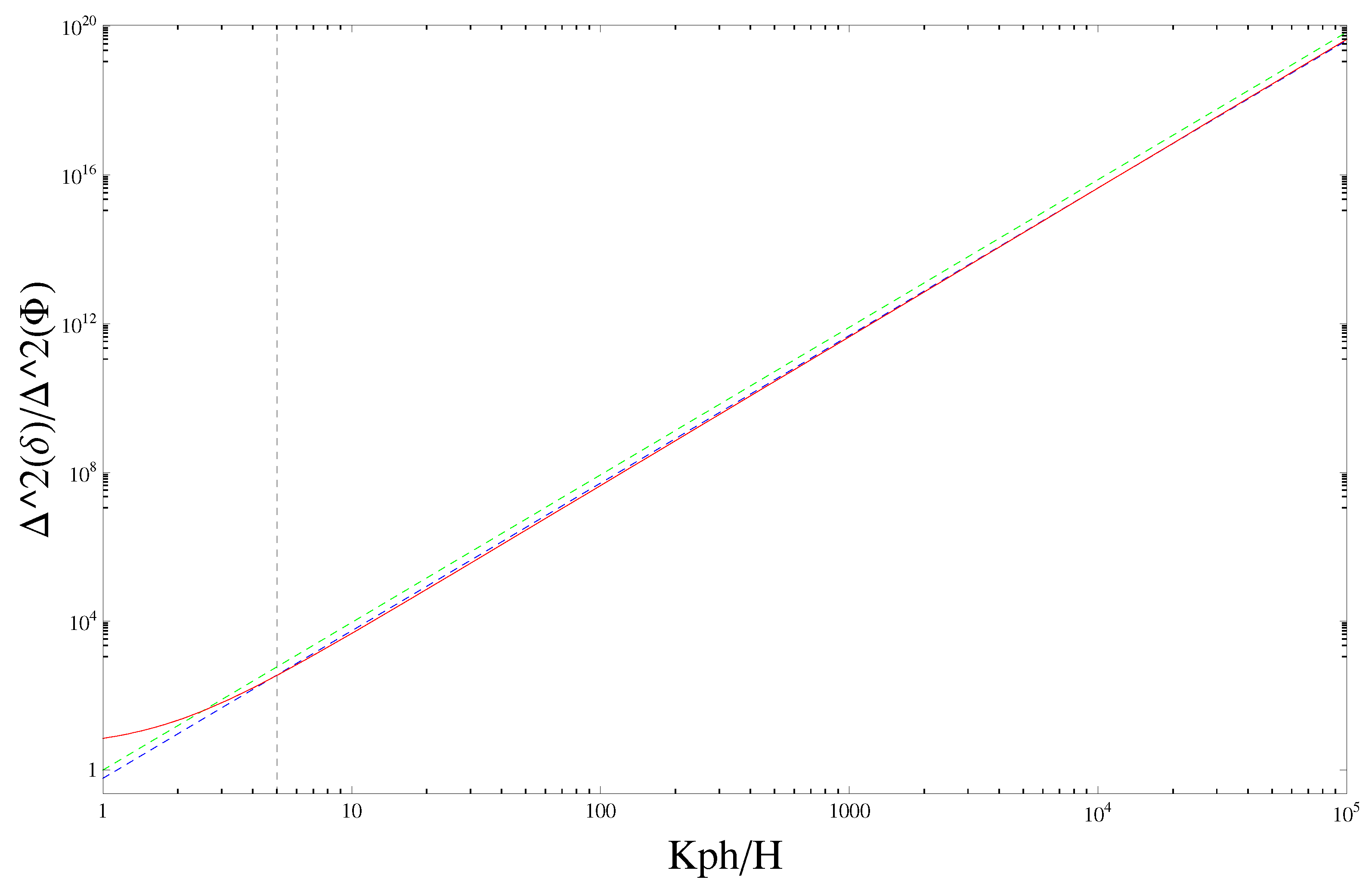
(see, e.g., [192], pp. 291, 292), where $n_s$ is the scalar spectral index [193]. Once again, we can test the validity of the polytropic DM model by reproducing the spectrum of rest-mass density perturbations in the associated $\Lambda$CDM-like limit. The reason is that most of the observational data accumulated so far are model dependent [175] and, currently, the most popular model is the so-called concordance, i.e., $\Lambda$CDM model [13]. Accordingly, as regards the dimensionless power spectrum of cosmological perturbations in the $\Lambda$CDM-like limit of the polytropic DM model under consideration, we have

$$\frac{{\Delta }^2\left(\delta \right)}{{\Delta }^2\left(\varphi \right)}=4{\left[1+\frac{1}{3}{\left(\frac{k_{ph}}{H}\right)}^2\right]}^2,$$

(63)

where $k_{ph}=k/S\left(t\right)$ is the associated physical wavenumber [162]. The behavior of Equation (63) as a function of $k_{ph}$ (in units of H) is depicted in Figure 6 (red solid line). Accordingly, we observe that for $\left(\frac{k_{ph}}{H}\right)\ge 5$, i.e., for every physical wavelength less than the horizon length (dashed verical line), the quantity ${\Delta }^2\left(\delta \right)/{\Delta }^2\left(\varphi \right)$ exhibits a prominent power-law dependence on $k_{ph}$, of the form

$$\frac{{\Delta }^2\left(\delta \right)}{{\Delta }^2\left(\varphi \right)}\sim {\left(\frac{k_{ph}}{H}\right)}^{3.970}$$

(64)

and, therefore,

$${\Delta }^2\left(\varphi \right)\sim \frac{{\Delta }^2\left(\delta \right)}{{\left(\frac{k_{ph}}{H}\right)}^{3.970}}=\frac{{\left(\frac{k_{ph}}{H}\right)}^{n_s+3}}{{\left(\frac{k_{ph}}{H}\right)}^{3.970}}={\left(\frac{k_{ph}}{H}\right)}^{n_s-0.970}.$$

(65)

CMB anisotropy measurements (see, e.g., [52,53]) and several physical arguments (see, e.g., [189], p. 466, [192], p. 292) suggest that the power spectrum of metric perturbations is scale invariant, i.e., ${\Delta }^2\left(\varphi \right)\sim k^0$. In this case, Equation (65) yields

$$n_s=0.970.$$

(66)

In view of Equations (62) and (66), we see that, although in principle there is no reason why the rest-mass density spectrum should exhibit a power-law behavior, in the context of the polytropic DM model it effectively does so, i.e.,

$${\Delta }^2\left(\delta \right)\sim k_{ph}^{3+n_s^{eff}},\mathrm{with}{n}_s^{eff}=0.970.$$

(67)

What is more important is that the theoretically derived value (67) for the effective scalar spectral index of rest-mass density perturbations in the $\Lambda$CDM-like limit of the polytropic DM model actually reproduces the corresponding observational (i.e., Planck) result, $n_s^{obs}=0.968\pm 0.006$ [55,56]. In short, matter perturbations of linear dimensions smaller than the Hubble radius, when considered in the $\Lambda$CDM-like (i.e., $\Gamma =0$) limit of the polytropic DM model under consideration, effectively exhibit a power-law behavior of the form ${\left|\delta \right|}^2\sim k^{n_s^{eff}}$, with the associated scalar spectral index being equal to $n_s^{eff}=0.970$, i.e., very close to observation.

3.10. Rest-Mass Energy–DE Equality

In view of Equation (19), the rest-mass energy density, ${\epsilon }_{mat}=\rho c^2$, and the internal (dark) energy density, ${\epsilon }_{int}=\epsilon -{\epsilon }_{mat}$, of the polytropic DM model under consideration satisfy the relation

$$\frac{{\epsilon }_{int}}{{\epsilon }_{mat}}=\frac{1-{\Omega }_M}{{\Omega }_M}\frac{1}{{(1+z)}^{3(1-\Gamma )}}.$$

(68)

Equation (68) suggests that, for $\Gamma =0$, DE becomes equal to its rest-mass counterpart, not at transition $(z_{tr}=0.744)$ but quite later, at $z_{eq}=0.384$, which is very close to the corresponding observationally determined value $z_{eq}=0.391\pm 0.033$ [29], associated (once again) with the $\Lambda$CDM model.

3.11. It Is Not a Coincidence

The evolution of a spatially flat FRW model is governed by Equations (5), (6), and (8). The combination of them results in

$$\frac{\ddot{S}}{S}=-\frac{4\pi G}{3c^2}\left(ϵ+3p\right)$$

(69)

(see, e.g., [43,44]); hence, the condition for accelerated expansion, $\ddot{S}>0$, yields

$$\epsilon +3p<0.$$

(70)

In the context of the polytropic DM model, condition (70) is written in the form

$${\rho }_0{c}^2{(1+z)}^3\left[1-(2+3|\Gamma \left|\right)\frac{1-{\Omega }_M}{{\Omega }_M}\frac{1}{{(1+z)}^{3(1+|\Gamma \left|\right)}}\right]<0,$$

(71)

in view of which such a model accelerates its expansion at cosmological redshifts lower than a particular value, namely,

$$z<{\left[(2+3|\Gamma \left|\right)\frac{1-{\Omega }_M}{{\Omega }_M}\right]}^{\frac{1}{3(1+|\Gamma \left|\right)}}-1\equiv z_{tr},$$

(72)

in complete correspondence with Equation (34). According to Equations (70) and (72), the assumption that the cosmological evolution can be driven by a polytropic DM fluid could most definitely explain why the universe transits from deceleration to acceleration at $z_{tr}$, without the need for any novel DE component or the cosmological constant. Instead, it would reveal a conventional form of DE, i.e., the one due to this fluid’s internal motions, which, so far, has been disregarded [113].

4. Discussion and Conclusions

The possibility that the extra DE needed to compromise both spatial flatness and the accelerated expansion of the universe actually corresponds to the thermodynamic internal energy of the cosmic fluid itself is reviewed and scrutinized. In this approach, the universe is filled with a perfect fluid of collisional DM, the volume elements of which perform polytropic flows [160,161,162,163]. In the distant past $(z\gg 1)$ the polytropic DM model so assumed behaves as an EdS model, filled with dust (cf. Equation (32)), while, on the approach to the present epoch $(t\simeq 0.75t_0)$, the internal physical characteristics of the cosmic fluid take over its dynamics (cf. Equation 68). Their energy can compensate the DE needed to compromise spatial flatness (cf. Equation (20)), while the associated cosmic pressure is negative (cf. Equation (18)). As a consequence, the polytropic DM model under consideration accelerates its expansion at cosmological redshifts lower than a transition value (cf. Equation (34)), in consistency with condition $\epsilon +3p<0$ (cf. Equation (72)). This model is characterized by a free parameter, the associated polytropic exponent $\Gamma$. In fact, several physical arguments can impose successive constraints on $\Gamma$, which, eventually, settles down to the range $-0.1<\Gamma \le 0$ (cf. Equation (44)); namely, if it is not zero (i.e., a $\Lambda$CDM-like model), it is definitely negative and very close to zero.

The polytropic DM model under consideration can reproduce all the major observational results of conventional (i.e., $\Lambda$CDM) cosmology, simply by means of a single fluid, i.e., without a priori assuming the existence of any DE component and/or the cosmological constant. This model actually belongs to the broad class of the unified DE models, in which the DE effects are due to the particular properties of the (unique) cosmic fluid (in connection, see, e.g., [194,195]).

We can test the validity of the polytropic DM model so assumed, by reproducing all the current cosmological issues in the associated $\Lambda$CDM-like limit. The reason is that, most of the observational data accumulated so far are model dependent [175] and, currently, the most popular model is the $\Lambda$CDM model. In this context, our polytropic DM model can confront all major issues of cosmological significance, such as, e.g.:

• The nature of the universal (dark) energy deficit needed to compromise spatial flatness: In the polytropic DM model under consideration it can be attributed to thermodynamic energy of the associated fluid internal motions (cf. Equations (19) and (20)).
• The accelerated expansion of the universe: For $t>0.75t_0$ (i.e., quite close to the present epoch), the solution of the Friedmann equation that governs the evolution of the scale factor, $S\left(t\right)$, in the polytropic DM model, becomes concave, i.e., $\ddot{S}>0$ resulting in the acceleration of the universe expansion (see, e.g., Figure 1).
• The age problem: For every $-0.1<\Gamma \le 0$, the age of the polytropic DM model, $t_0$, is always larger than that of its EdS counterpart, $t_{EdS}=\frac{2}{3H_0}$. In the $\Lambda$CDM-like $(\Gamma =0)$ limit, we obtain $t_0=1.483t_{EdS}=13.79Gys$, in complete agreement with the corresponding observational result [55,56,57] for the age of the $\Lambda$CDM universe (see, e.g., Figure 2).
• The value of the cosmological redshift parameter at which transition from deceleration to acceleration takes place, $z_{tr}$: In the $\Lambda$CDM-like limit (i.e., $\Gamma =0$) of the polytropic DM model so assumed, we obtain $z_{tr}=0.744$ (cf. Figure 3), which lies well within range of the corresponding $\Lambda$CDM result, namely, $z_{tr}=0.752\pm 0.041$ [29], as well as in the associated model-independent range $z_{tr}=0.{739}_{-0.089}^{+0.065}$ [181].
• The long-sought theoretical value of the deceleration parameter, q, at the present epoch: In the $\Lambda$CDM-like limit of the polytropic DM model under consideration, $q_0=-0.54$ (cf. Equation (33), for $\Gamma =0$), that is fully compatible with the observational result, $q_0=-0.{53}_{-0.13}^{+0.17}$ [179], associated with the $\Lambda$CDM model.
• The behavior of the total EoS parameter, w: In the $\Lambda$CDM-like (i.e., $\Gamma =0$) limit of the polytropic DM model, today, $w_{tot}\approx -0.7$ (cf. Figure 4), while, as z grows, $w_{tot}\to 0$, as suggested by $\Lambda$CDM cosmology [88].
• The resulting range of values of the polytropic index, $-0.1<\Gamma \le 0$: It is in excellent agreement with the associated result for a generalized Chaplygin gas, $p\sim -{\rho }^{\alpha }$, arising from the combination of X-ray and SNe Ia measurements with data from Fanaroff–Riley type IIb radio-galaxies, namely, $\alpha =-0.{09}_{-0.33}^{+0.54}$ [184].
• The behavior of the associated jerk parameter, $j\left(z\right)$: The polytropic DM model possesses a positive jerk parameter, with the aid of which (at transition) we can also estimate the value of the polytropic index, $|\Gamma |$, in a model-independent manner [181], namely, $|\Gamma |\in (0.02,0.03)$.
• The Hubble diagram of the SNe Ia standard candles: In the polytropic DM model under consideration, the theoretically derived distance modulus fits the entire Union 2.1 dataset [29] with accuracy. In other words, there is absolutely no disagreement between the theoretical prediction of our model and the observed distribution of the distant SNe Ia events (cf. Figure 5).
• The CMB shift parameter: In the $\Lambda$CDM-like limit of the polytropic DM model, $\mathcal{R}=1.7342$, while, according to the nine-year WMAP survey, the value of the CMB shift parameter in the standard $\Lambda$CDM model is $\mathcal{R}=1.7329\pm 0.0058$ [191]. In other words, the value of the CMB shift parameter in the $\Lambda$CDM-like limit of the polytropic DM model actually reproduces the corresponding result obtained by fitting the CMB data to the standard $\Lambda$CDM model. It is, therefore, expected that, in the limit $\Gamma =0$, the polytropic DM model under consideration may very well also reproduce the observed CMB spectrum.
• Furthermore, in fact, it actually does so (cf. Equation (67)), since the theoretically derived value for the effective scalar spectral index of rest-mass density perturbations in the $\Lambda$CDM-like limit of the polytropic DM model, $n_s^{eff}=0.970$, actually reproduces the corresponding observational Planck result, $n_s^{obs}=0.968\pm 0.006$ [55,56]. In other words, matter perturbations of linear dimensions smaller than the horizon length, when considered in the $\Lambda$CDM-like (i.e., $\Gamma =0$) limit of a polytropic DM model, effectively exhibit a power-law behavior of the form ${\left|\delta \right|}^2\sim k^{n_s^{eff}}$, with the associated scalar spectral index being equal to $n_s^{eff}=0.970$, i.e., very close to observation.
• The rest-mass energy–DE equality: In the $\Lambda$CDM-like limit of the polytropic DM model under consideration (cf. Equation (68)), DE becomes equal to its rest-mass counterpart at $z_{eq}=0.384$, which is remarkably close to the corresponding observationally determined value $z_{eq}=0.391\pm 0.033$ [29], associated with the $\Lambda$CDM model.
• Finally, the polytropic DM model can, most definitely, explain why the universe transits to acceleration at $z_{tr}$, without the need for any novel DE component or the cosmological constant, solely being consistent with the general relativistic condition that $\epsilon +3p<0$ (cf. Equations (70) and (72)).

Compatibility of the polytropic DM model with the observational constraints on all the parameters of cosmological significance needs to be further explored and scrutinized, in order to decide on the likelihood of this model over all other alternatives and, especially, the $\Lambda$CDM model. Clearly, the ultimate verification of any (unified or not) DE model would be the reproduction of the observed DM halo distributions and the associated galactic evolution. In this context, preliminary results regarding the evolution of small-scale density perturbations at low redshift values suggest that, in the $c_s^2\ne 0$ case of the polytropic DM model, the density-contrast profile, $\delta \left(z\right)$, consists of peaks and troughs that resemble the observed galaxy distribution (in terms of z). Therefore, as regards the evolution of small-scale density perturbations in a polytropic DM model with $c_s^2\ne 0$, a more elaborated study is necessary and it will be the scope of a future work.

Finally, it is clear that this review article neither deals with nor takes into account the fundamental nature of the polytropic DM constituents, i.e., the field nature of the cosmic fluid. In this context, recent studies suggest that certain barotropic fluids may arise naturally from a $k-$essence lagrangian, involving a self-interacting (real or complex) scalar field [196]. In direct connection to the quantum origin of the polytropic DM fluid, one should also address the origin of the (extra) amount of heat, $\mathcal{C}dT$, offered to the volume elements, as suggested by Equation (7). According to [76], this could be due to a long-range confining force between the DM particles. In our case, it would be of the form $F=-K{r}^{2+3|\Gamma |}$, where r is the radial distance and $K>0$ is a normalization constant (in connection, see Equations (80) and (89) of [76]). This force may be either of gravitational origin or a new force [141,144]. In any case, it is not yet clear whether a system subject to a long-range confining force can reach thermodynamic equilibrium; hence, this is also a matter of debate that must be addressed in future studies.

In any case, instead of treating any novel DE component and/or modified gravity theories as pillars of contemporary cosmology, let us address a much simpler possibility: the polytropic flow of the conventional matter–energy content of the universe, in connection to a potential self-interacting nature of DM [197]. As we have demonstrated in this review, the yet ignored thermodynamical content of the universe could arise as a mighty and relatively inexpensive contestant for an extra (dark) energy candidate that could compensate both spatial flatness and accelerated expansion. In view of all the above, the cosmological model with matter content in the form of a self-interacting DM fluid whose volume elements perform polytropic flows looks very promising and should be further explored and scrutinized in the search for a viable alternative to the $\Lambda$CDM model.

References

- Turner, M.S.; White, M. CDM models with a smooth component. Phys. Rev. D 1997, 56, 4439–4443. [Google Scholar] [CrossRef] [Green Version]
- Perlmutter, S.; Turner, M.S.; White, M. Constraining dark energy with Type Ia Supernovae and large-scale structure. Phys. Rev. Lett. 1999, 83, 670–673. [Google Scholar] [CrossRef] [Green Version]
- Hamuy, M.; Phillips, M.M.; Suntzeff, N.B.; Schommer, R.A.; Maza, J.; Antezan, A.R.; Wischnjewsky, M.; Valladares, G.; Muena, C.; Gonzales, L.E.; et al. BVRI light curves for 29 Type IA Supernovae. Astronom. J. 1996, 112, 2408. [Google Scholar] [CrossRef] [Green Version]
- Garnavich, P.M.; Jha, S.; Challis, P.; Clocchiatti, A.; Diercks, A.; Filippenko, V.A.; Gilliland, R.L.; Hogan, C.J.; Kirshner, R.P.; Leibundgut, B.; et al. Supernova limits on the cosmic equation of state. Astrophys. J. 1998, 509, 74–79. [Google Scholar] [CrossRef] [Green Version]
- Perlmutter, S.; Aldering, G.; Valle, M.D.; Deustua, S.; Ellis, R.S.; Fabbro, S.; Fruchter, A.; Goldhaber, G.; Groom, D.E.; Hook, I.M.; et al. Discovery of a Supernova explosion at half the age of the Universe. Nature 1998, 391, 51. [Google Scholar] [CrossRef] [Green Version]
- Perlmutter, S.; Aldering, G.; Goldhaber, G.; Knop, R.A.; Nugent, P.; Castro, P.G.; Deustua, S.; Fabbro, S.; Goobar, A.; Groom, D.E.; et al. Measurements of Ω and Λ from 42 high-redshift Supernovae. Astrophys. J. 1999, 517, 565–586. [Google Scholar] [CrossRef]
- Schmidt, B.P.; Suntzeff, N.B.; Phillips, M.M.; Schommer, R.A.; Clocchiatti, A.; Kirshner, R.P.; Garnavich, P.; Challis, P.; Leibundgut, B.; Spyromilio, J.; et al. The High-Z Supernova search: Measuring cosmic deceleration and global curvature of the Universe using Type Ia Supernovae. Astrophys. J. 1998, 507, 46–63. [Google Scholar] [CrossRef]
- Riess, A.G.; Filippenko, A.V.; Challis, P.; Clocchiatti, A.; Diercks, A.; Garnavich, P.M.; Gilliland, R.L.; Hogan, C.J.; Jha, S.; Kirshner, R.P.; et al. Observational evidence from Supernovae for an accelerating Universe and a Cosmological Constant. Astronom. J. 1998, 116, 1009–1038. [Google Scholar] [CrossRef] [Green Version]
- Riess, A.G.; Nugent, P.E.; Gilliland, R.L.; Schmidt, B.P.; Tonry, J.; Dickinson, M.; Thompson, R.I.; Budavári, T.; Casertano, S.; Evans, A.S.; et al. The farthest known Supernova: Support for an accelerating Universe and a glimpse of the epoch of deceleration. Astrophys. J. 2001, 560, 49–71. [Google Scholar] [CrossRef] [Green Version]
- Riess, A.G.; Strolger, L.-G.; Tonry, J.; Casertano, S.; Ferguson, H.C.; Mobasher, B.; Challis, P.; Filippenko, A.V.; Jha, S.; Li, W.; et al. Type Ia Supernova discoveries at z>1 from the Hubble Space Telescope: Evidence for past deceleration and constraints on dark energy evolution. Astrophys. J. 2004, 607, 665–687. [Google Scholar] [CrossRef]
- Riess, A.G.; Strolger, L.-G.; Casertano, S.; Ferguson, H.C.; Mobasher, B.; Gold, B.; Challis, P.J.; Filippenko, A.V.; Jha, S.; Li, W.; et al. New Hubble Space Telescope discoveries of Type Ia Supernovae at z≥1: Narrowing constraints on the early behavior of dark energy. Astrophys. J. 2007, 659, 98–121. [Google Scholar] [CrossRef] [Green Version]
- Knop, R.A.; Aldering, G.; Amanullah, R.; Astier, P.; Blanc, G.; Burns, M.S.; Conley, A.; Deustua, S.E.; Doi, M.; Ellis, R.; et al. New constraints on ΩM, ΩΛ, and w from an independent set of 11 high-redshift Supernovae observed with the Hubble Space Telescope. Astrophys. J. 2003, 598, 102–137. [Google Scholar] [CrossRef] [Green Version]
- Tonry, J.L.; Schmidt, B.P.; Barris, B.; Candia, P.; Challis, P.; Clocchiatti, A.; Coil, A.L.; Filippenko, A.V.; Garnavich, P.; Hogan, C.; et al. Cosmological results from high-z Supernovae. Astrophys. J. 2003, 594, 1–24. [Google Scholar] [CrossRef] [Green Version]
- Barris, B.; Tonry, J.L.; Blondin, S.; Challis, P.; Chornock, R.; Clocchiatti, A.; Filippenko, A.V.; Garnavich, P.; Holland, S.T.; Jha, S.; et al. Twenty-three high-redshift Supernovae from the institute for Astronomy Deep Survey: Doubling the Supernova sample at z>0.7. Astrophys. J. 2004, 602, 571–594. [Google Scholar] [CrossRef] [Green Version]
- Krisciunas, K.; Garnavich, P.M.; Challis, P.; Prieto, J.L.; Riess, A.G.; Barris, B.; Aguilera, C.; Becker, A.C.; Blondin, S.; Chornock, R.; et al. Hubble Space Telescope observations of nine high-redshift ESSENCE Supernovae. Astronom. J. 2005, 130, 2453–2472. [Google Scholar] [CrossRef]
- Astier, P.; Guy, J.; Regnault, N.; Pain, R.; Aubourg, E.; Balam, D.; Basa, S.; Carlberg, R.G.; Fabbro, S.; Fouchez, D.; et al. The Supernova Legacy Survey: Measurement of ΩM, ΩΛ and w from the first year data set. A&A 2006, 447, 31–48. [Google Scholar]
- Jha, S.; Kirshner, R.P.; Challis, P.; Garnavich, P.M.; Matheson, T.; Soderberg, A.M.; Graves, G.J.M.; Hicken, M.; Alves, J.F.; Arce, H.G.; et al. UBVRI light curves of 44 Type Ia Supernovae. Astronom. J. 2006, 131, 527–554. [Google Scholar] [CrossRef] [Green Version]
- Miknaitis, G.; Pignata, G.; Rest, A.; Wood-Vasey, W.M.; Blondin, S.; Challis, P.; Smith, R.C.; Stubbs, C.W.; Suntzeff, N.B.; Foley, R.J.; et al. The ESSENCE Supernova Survey: Survey optimization, observations and Supernova photometry. Astrophys. J. 2007, 666, 674–693. [Google Scholar] [CrossRef]
- Wood-Vasey, W.M.; Miknaitis, G.; Stubbs, C.W.; Jha, S.; Riess, A.G.; Garnavich, P.M.; Kirshner, R.P.; Aguilera, C.; Becker, A.C.; Blackman, J.W.; et al. Observational constraints on the nature of dark energy: First cosmological results from the ESSENCE Supernova survey. Astrophys. J. 2007, 666, 694–715. [Google Scholar] [CrossRef]
- Amanullah, R.; Stanishev, V.; Goobar, A.; Schahmaneche, K.; Astier, P.; Balland, C.; Ellis, R.S.; Fabbro, S.; Hardin, D.; Hook, I.M.; et al. Light curves of five Type Ia Supernovae at intermediate redshift. A&A 2008, 486, 375–382. [Google Scholar]
- Amanullah, R.; Lidman, C.; Rubin, D.; Aldering, G.; Astier, P.; Barbary, K.; Burns, M.S.; Conley, A.; Dawson, K.S.; Deustua, S.E.; et al. Spectra and Hubble Space Telescope light curves of six Type Ia Supernovae at 0.511<z<1.12 and the Union 2 Compilation. Astrophys. J. 2010, 716, 712–738. [Google Scholar]
- Holtzman, J.A.; Marriner, J.; Kessler, R.; Sako, M.; Dilday, B.; Frieman, J.A.; Schneider, D.P.; Bassett, B.; Becker, A.; Cinabro, D.; et al. The Sloan Digital Sky Survey-II: Photometry and Supernova IA light curves from the 2005 data. Astronom. J. 2008, 136, 2306–2320. [Google Scholar] [CrossRef]
- Kowalski, M.; Rubin, D.; Aldering, G.; Agostinho, R.J.; Amadon, A.; Amanullah, R.; Balland, C.; Barbary, K.; Blanc, G.; Challis, P.J.; et al. Improved cosmological constraints from new, old and combined Supernova data sets. Astrophys. J. 2008, 686, 749–778. [Google Scholar] [CrossRef]
- Hicken, M.; Challis, P.; Jha, S.; Kirshner, R.P.; Matheson, T.; Modjaz, M.; Rest, A.; Wood-Vasey, W.M.; Bakos, G.; Barton, E.J.; et al. CfA3: 185 Type Ia Supernova light curves from the CfA. Astrophys. J. 2009, 700, 331–357. [Google Scholar] [CrossRef]
- Hicken, M.; Wood-Vasey, M.; Blondin, S.; Chalis, P.; Jha, S.; Kelly, P.L.; Rest, A.; Kirshner, R.P. Improved dark energy constraints from ∼100 new CfA Supernova Type Ia light curves. Astrophys. J. 2009, 700, 1097–1140. [Google Scholar] [CrossRef] [Green Version]
- Kessler, R.; Becker, A.C.; Cinabro, D.; Vanderplas, J.; Frieman, J.A.; Marriner, J.; Davis, T.M.; Dilday, B.; Holtzman, J.; Jha, S.W.; et al. First-Year Sloan Digital Sky Survey-II Supernova results: Hubble diagram and cosmological parameters. Astroph. J. Sup. Series 2009, 185, 32–84. [Google Scholar] [CrossRef]
- Contreras, C.; Hamuy, M.; Phillips, M.M.; Folatelli, G.; Suntzeff, N.B.; Persson, S.E.; Stritzinger, M.; Boldt, L.; González, S.; Krzeminski, W.; et al. The Carnegie Supernova Project: First photometry data release of low-redshift Type Ia Supernovae. Astronom. J. 2010, 139, 519–539. [Google Scholar] [CrossRef] [Green Version]
- Guy, J.; Sullivan, M.; Conley, A.; Regnault, N.; Astier, P.; Balland, C.; Basa, S.; Carlberg, R.G.; Fouchez, D.; Hardin, D.; et al. The Supernova Legacy Survey 3-year sample: Type Ia Supernovae photometric distances and cosmological constraints. A&A 2010, 523, A7. [Google Scholar]
- Suzuki, N.; Rubin, D.; Lidman, C.; Aldering, G.; Amanullah, R.; Barbary, K.; Barrientos, L.F.; Botyanszki, J.; Brodwin, M.; Connolly, N.; et al. The Hubble Space Telescope Cluster Supernova survey. V. Improving the dark energy constraints above z>1 and building an early-type-hosted Supernova sample. Astrophys. J. 2012, 746, A85. [Google Scholar] [CrossRef] [Green Version]
- Scolnic, D.M.; Jones, D.O.; Rest, A.; Pan, Y.C.; Chornock, R.; Foley, R.J.; Huber, M.E.; Kessler, R.; Narayan, G.; Riess, A.G.; et al. The complete light-curve sample of spectroscopically confirmed SNe Ia from Pan-STARRS1 and cosmological constraints from the combined Pantheon Sample. Astrophys. J. 2018, 859, 101. [Google Scholar] [CrossRef]
- Abbott, T.M.C.; Allam, S.; Andersen, P.; Angus, C.; Asorey, J.; Avelino, A.; Avila, S.; Bassett, B.A.; Bechtol, K.; Bernstein, G.M.; et al. First cosmology results using type Ia supernovae from the dark energy survey: Constraints on cosmological. Astrophys. J. Lett. 2019, 872, L30. [Google Scholar] [CrossRef]
- Carroll, S.M.; Press, W.H.; Turner, E.L. The cosmological constant. ARA&A 1992, 30, 499–542. [Google Scholar]
- Sahni, V.; Starobinsky, A. The case for a positive cosmological Λ-term. IJMP D 2000, 9, 373–443. [Google Scholar] [CrossRef]
- Allen, S.W.; Schmidt, R.W.; Ebeling, H.; Fabian, A.C.; van Speybroeck, L. Constraints on dark energy from Chandra observations of the largest relaxed galaxy clusters. MNRAS 2004, 353, 457–467. [Google Scholar] [CrossRef] [Green Version]
- Boughn, S.; Crittenden, R. A correlation between the cosmic microwave background and large-scale structure in the Universe. Nature 2004, 427, 45–47. [Google Scholar] [CrossRef]
- Eisenstein, D.J.; Zehavi, I.; Hogg, D.W.; Scoccimarro, R.; Blanton, M.R.; Nichol, R.C.; Scranton, R.; Seo, H.-J.; Tegmark, M.; Zheng, Z.; et al. Detection of the baryon acoustic peak in the large-scale correlation function of SDSS luminous red galaxies. Astrophys. J. 2005, 633, 560–574. [Google Scholar] [CrossRef]
- Percival, W.J.; Reid, B.A.; Eisenstein, D.J.; Bahcall, N.A.; Budavari, T.; Frieman, J.A.; Fukugita, M.; Gunn, J.E.; Ivezic, Z.; Knapp, G.R.; et al. Baryon acoustic oscillations in the Sloan Digital Sky Survey data release 7 galaxy sample. MNRAS 2010, 401, 2148–2168. [Google Scholar] [CrossRef] [Green Version]
- Huterer, D. Weak lensing and dark energy. Phys. Rev. D 2002, 65, 063001. [Google Scholar] [CrossRef] [Green Version]
- Copeland, E.J.; Sami, M.; Tsujikawa, S. Dynamics of Dark Energy. IJMP D 2006, 15, 1753–1935. [Google Scholar] [CrossRef] [Green Version]
- Seljak, U.; Slosar, A.; McDonald, P. Cosmological parameters from combining the Lyman-α forest with CMB, galaxy clustering and SN constraints. J. Cosmol. Astropart. Phys. 2006, 10, A014. [Google Scholar] [CrossRef]
- Sahni, V. Dark matter and dark energy. In The Physics of the Early Universe; Papantonopoulos, L., Ed.; Lecture Notes in Physics 653; Springer: Berlin/Heidelberg, Germany, 2004; p. 141. [Google Scholar]
- Frieman, J.A.; Turner, M.S.; Huterer, D. Dark Energy and the Accelerating Universe. Ann. Rev. Astron. Astrophys. 2008, 46, 385. [Google Scholar] [CrossRef] [Green Version]
- Linder, E.V. Mapping the cosmological expansion. Rep. Prog. Phys. 2008, 71, 056901. [Google Scholar] [CrossRef]
- Caldwell, R.R.; Kamionkowski, M. The Physics of Cosmic Acceleration. Annual Rev. Nucl. Part. Sci. 2009, 59, 397–429. [Google Scholar] [CrossRef] [Green Version]
- de Bernardis, P.; Ade, P.A.R.; Bock, J.J.; Bond, J.R.; Borrill, J.; Boscaleri, A.; Coble, K.; Crill, B.P.; De Gasperis, G.; Farese, P.C.; et al. A flat Universe from high-resolution maps of the cosmic microwave background radiation. Nature 2000, 404, 955–959. [Google Scholar] [CrossRef] [PubMed] [Green Version]
- Jaffe, A.H.; Ade, P.A.R.; Balbi, A.; Bock, J.J.; Bond, J.R.; Borrill, J.; Boscaleri, A.; Coble, K.; Crill, B.P.; de Bernardis, P.; et al. Cosmology from MAXIMA-1, BOOMERANG and COBE DMR cosmic microwave background observations. Phys. Rev. Lett. 2001, 86, 3475–3479. [Google Scholar] [CrossRef]
- Padin, S.; Cartwright, J.K.; Mason, B.S.; Pearson, T.J.; Readhead, A.C.S.; Shepherd, M.C.; Sievers, J.; Udomprasert, P.S.; Holzapfel, W.L.; Myers, S.T.; et al. First intrinsic anisotropy observations with the Cosmic Background Imager. Astrophys. J. 2001, 549, L1–L5. [Google Scholar] [CrossRef] [Green Version]
- Stompor, R.; Abroe, M.; Ade, P.; Balbi, A.; Barbosa, D.; Bock, J.; Borrill, J.; Boscaleri, A.; de Bernardis, P.; Ferreira, P.G.; et al. Cosmological implications of the MAXIMA-1 high-resolution cosmic microwave background anisotropy measurement. Astrophys. J. 2001, 561, L7–L10. [Google Scholar] [CrossRef] [Green Version]
- Netterfield, C.B.; Ade, P.; Bock, J.J.; Bond, J.R.; Borrill, J.; Boscaleri, A.; Coble, K.; Contaldi, C.R.; Crill, B.P.; de Bernardis, P.; et al. A measurement by BOOMERANG of multiple peaks in the angular power spectrum of the cosmic microwave background. Astrophys. J. 2002, 571, 604–614. [Google Scholar] [CrossRef]
- Spergel, D.N.; Verde, L.; Peiris, H.V.; Komatsu, E.; Nolta, M.R.; Bennett, C.L.; Halpern, M.; Hinshaw, G.; Jarosik, N.; Kogut, A.; et al. First-year Wilkinson Microwave Anisotropy Probe (WMAP) observations: Determination of cosmological parameters. Astrophys. J. Suppl. Series 2003, 148, 175–194. [Google Scholar] [CrossRef] [Green Version]
- Spergel, D.N.; Bean, R.; Dore, O.; Nolta, M.R.; Bennett, C.L.; Dunkley, J.; Hinshaw, G.; Jarosik, N.; Komatsu, E.; Page, L.; et al. Three-year Wilkinson Microwave Anisotropy Probe (WMAP) observations: Implications for Cosmology. Astrophys. J. Suppl. Series 2007, 170, 377–408. [Google Scholar] [CrossRef] [Green Version]
- Komatsu, E.; Dunkley, J.; Nolta, M.R.; Bennett, C.L.; Gold, B.; Hinshaw, G.; Jarosik, N.; Larson, D.; Limon, M.; Page, L.; et al. Five-year Wilkinson Microwave Anisotropy Probe observations: Cosmological interpretation. Astrophys. J. Suppl. Series 2009, 180, 330–376. [Google Scholar] [CrossRef] [Green Version]
- Komatsu, E.; Smith, K.M.; Dunkley, J.; Bennett, C.L.; Gold, B.; Hinshaw, G.; Jarosik, N.; Larson, D.; Nolta, M.R.; Page, L.; et al. Seven-year Wilkinson Microwave Anisotropy Probe (WMAP) observations: Cosmological interpretation. Astrophys. J. Suppl. Series 2011, 192, A18. [Google Scholar] [CrossRef] [Green Version]
- Hinshaw, G.; Larson, D.; Komatsu, E.; Spergel, D.N.; Bennett, C.L.; Dunkley, J.; Nolta, M.R.; Halpern, M.; Hill, R.S.; Odegard, N.; et al. Nine-year Wilkinson Microwave Anisotropy Probe (WMAP) observations: Cosmological parameter results. Astrophys. J. Suppl. 2013, 208, A19. [Google Scholar] [CrossRef] [Green Version]
- Ade, P.A.R. [Planck Collaboration] 2015 Results XVIII: Cosmolological parameters. Astron. Astrophys. 2016, 594, A18. [Google Scholar]
- Ade, P.A.R. [Planck Collaboration] 2018 Results IX: Cosmological parameters. Astron. Astrophys. 2020, 641, A9. [Google Scholar]
- Abbott, T.M.C.; Aguena, M.; Alarcon, A.; Allam, S.; Alves, O.; Amon, A.; Andrade-Oliveira, F.; Annis, J.; Avila, S.; Bacon, D.; et al. Dark Energy Survey Year 3 Results: Cosmological Constraints from Galaxy Clustering and Weak Lensing. arXiv 2021, arXiv:2105.13549. [Google Scholar]
- Padmanabhan, T. Cosmological constant–the weight of the vacuum. Phys. Rep. 2003, 380, 235–320. [Google Scholar] [CrossRef] [Green Version]
- Caldwell, R.R.; Dave, R.; Steinhardt, P.J. Cosmological imprint of an energy component with general equation of state. Phys. Rev. Lett. 1998, 80, 1582–1585. [Google Scholar] [CrossRef]
- Armendariz-Picon, C.; Mukhanov, V.F.; Steinhardt, P.J. Essentials of k-essence. Phys. Rev. D 2001, 63, 103510. [Google Scholar] [CrossRef]
- Caldwell, R.R. A phantom menace? Cosmological consequences of a dark energy component with super-negative equation of state. Phys. Lett. B 2002, 545, 23–29. [Google Scholar] [CrossRef] [Green Version]
- Padmanabhan, T. Accelerated expansion of the Universe driven by tachyonic matter. Phys. Rev. D 2002, 66, 021301. [Google Scholar] [CrossRef] [Green Version]
- Dvali, G.R.; Gabadadze, G.; Porratti, M. 4D gravity on a brane in 5D Minkowski space. Phys. Lett. B 2000, 485, 208–214. [Google Scholar] [CrossRef] [Green Version]
- Bousso, R.; Polchinski, J. Quantization of four-form fluxes and dynamical neutralization of the Cosmological Constant. JHEP 2000, 6, A006. [Google Scholar] [CrossRef]
- Esposito-Farese, G.; Polarski, D. Scalar-tensor gravity in an accelerating Universe. Phys. Rev. D 2001, 63, 063504. [Google Scholar] [CrossRef] [Green Version]
- Capozziello, S.; Carloni, S.; Troisi, A. Quintessence without scalar fields. Recent Res. Dev. Astron. Astrophys. 2003, 1, 625–671. [Google Scholar]
- Nojiri, S.; Odintsov, S.D.; Oikonomou, V.K. Modified gravity theories on a nutshell: Inflation, bounce, and late-time evolution. Phys. Rep. 2017, 692, 1–104. [Google Scholar] [CrossRef] [Green Version]
- Cohen, A.G.; Kaplan, D.M.; Nelson, A.G. Effective Field Theory, Black Holes, and the Cosmological Constant. Phys. Rev. Lett. 1999, 82, 4971–4974. [Google Scholar] [CrossRef] [Green Version]
- Li, M. A model of holographic dark energy. Phys. Lett. B 2004, 603, 1–5. [Google Scholar] [CrossRef]
- Pavón, D.; Zimdahl, W. Holographic dark energy and cosmic coincidence. Phys. Lett. B 2005, 628, 206–210. [Google Scholar] [CrossRef]
- Kamenshchik, A.; Moschella, U.; Pasquier, V. An alternative to quintessence. Phys. Lett. B 2001, 511, 265–268. [Google Scholar] [CrossRef] [Green Version]
- Bento, M.C.; Bertolami, O.; Sen, A.A. Generalized Chaplygin gas, accelerated expansio, and dark-energy-matter unification. Phys. Rev. D 2002, 66, 043507. [Google Scholar] [CrossRef] [Green Version]
- Bean, R.; Doré, O. Are Chaplygin gases serious contenders for the dark energy? Phys. Rev. D 2003, 68, 023515. [Google Scholar] [CrossRef] [Green Version]
- Sen, A.A.; Scherrer, R.J. Generalizing the generalized Chaplygin gas. Phys. Rev. D 2005, 72, 063511. [Google Scholar] [CrossRef] [Green Version]
- Freese, K.; Lewis, M. Cardassian expansion: A model in which the Universe is flat, matter dominated and accelerating. Phys. Lett. B 2002, 540, 1–8. [Google Scholar] [CrossRef] [Green Version]
- Gondolo, P.; Freese, K. Fluid interpretation of Cardassian expansion. Phys. Rev. D 2003, 68, 063509. [Google Scholar] [CrossRef] [Green Version]
- Wang, Y.; Freese, K.; Gondolo, P.; Lewis, M. Future Type Ia Supernova data as tests of dark energy from modified Friedmann equations. Astrophys. J. 2003, 594, 25–32. [Google Scholar] [CrossRef] [Green Version]
- Mongan, T.R. A Simple Quantum Cosmology. Gen. Relativ. Grav. 2001, 33, 1415–1424. [Google Scholar] [CrossRef] [Green Version]
- Deffayet, C.; Dvali, G.; Gabadadze, G. Accelerated Universe from gravity leaking to extra dimensions. Phys. Rev. D 2002, 65, 044023. [Google Scholar] [CrossRef] [Green Version]
- Perivolaropoulos, L. Equation of state of the oscillating Brans-Dicke scalar and extra dimensions. Phys. Rev. D 2003, 67, 123516. [Google Scholar] [CrossRef]
- Sami, M.; Savchenko, N.; Toporensky, A. Aspects of scalar field dynamics in Gauss–Bonnet brane worlds. Phys. Rev. D 2004, 70, 123528. [Google Scholar] [CrossRef] [Green Version]
- Fardon, R.; Nelson, A.E.; Weiner, N. Dark energy from mass varying neutrinos. JCAP 2004, 10, 005. [Google Scholar] [CrossRef] [Green Version]
- Peccei, R.D. Neutrino models of dark energy. Phys. Rev. D 2005, 71, 023527. [Google Scholar] [CrossRef] [Green Version]
- Buchert, T. 2000, On average properties of inhomogeneous fluids in General Relativity: Dust Cosmologies. Gen. Relativ. Gravit. 2000, 32, 105–126. [Google Scholar] [CrossRef] [Green Version]
- Kolb, E.W.; Matarrese, S.; Riotto, A. On cosmic acceleration without dark energy. New J. Phys. 2006, 8, 322. [Google Scholar] [CrossRef]
- Celerier, M.-N. The accelerated expansion of the Universe challenged by an effect of the inhomogeneities. A review. New Adv. Phys. 2007, 1, 29–50. [Google Scholar]
- Ellis, G.F.R. Dark energy and inhomogeneity. J. Phys. Conf. Ser. 2009, 189, 012011. [Google Scholar] [CrossRef]
- Miao, L.I.; Xiao-Dong, L.I.; Wang, S.; Wang, Y. Dark energy. Commun. Theor. Phys. 2011, 56, 525–604. [Google Scholar]
- Visser, M. Cosmography: Cosmology without the Einstein equations. Gen. Relat. Grav. 2005, 37, 1541–1548. [Google Scholar] [CrossRef] [Green Version]
- Cattoen, C.; Visser, M. Cosmography: Extracting the Hubble Series From the Supernova Data. arXiv 2007, arXiv:0703122[gr-qc]. [Google Scholar]
- Cattoen, C. The Hubble series: Convergence properties and redshift variables. Class. Quant. Grav. 2007, 24, 5985–5998. [Google Scholar] [CrossRef]
- Cattoen, C.; Visser, M. Cosmodynamics: Energy conditions, Hubble bounds, density bounds, time and distance bounds. Class. Quant. Grav. 2008, 25, 165013. [Google Scholar] [CrossRef] [Green Version]
- Vitagliano, V.; Xia, J.-Q.; Liberati, S.; Viel, M. High-redshift cosmography. JCAP 2010, 3, 005. [Google Scholar] [CrossRef]
- Luongo, O. Cosmography with the Hubble Parameter. Mod. Phys. Lett. A 2011, 26, 1459–1466. [Google Scholar] [CrossRef]
- Aviles, A.; Gruber, C.; Luongo, O.; Quevedo, H. Cosmography and constraints on the equation of state of the Universe in various parametrizations. Phys. Rev. D 2012, 86, 123516. [Google Scholar] [CrossRef] [Green Version]
- Bamba, K.; Capozziello, S.; Nojiri, S.; Odintsov, S.D. Dark energy cosmology: The equivalent description via different theoretical models and cosmography tests. Astrophys. Space Sci. 2012, 342, 155–228. [Google Scholar] [CrossRef] [Green Version]
- Demianski, M.; Piedipalumbo, E.; Rubano, C.; Scudellaro, P. High-redshift cosmography: New results and implications for dark energy. MNRAS 2012, 426, 1396–1415. [Google Scholar] [CrossRef] [Green Version]
- Shafieloo, A.; Kim, A.G.; Linder, E.V. Gaussian process cosmography. Phys. Rev. D 2012, 85, 123530. [Google Scholar] [CrossRef] [Green Version]
- Aviles, A.; Bravetti, A.; Capozziello, S.; Luongo, O. Updated constraints on f(R) gravity from cosmography. Phys. Rev. D 2013, 87, 044012. [Google Scholar] [CrossRef] [Green Version]
- Aviles, A.; Bravetti, A.; Capozziello, S.; Luongo, O. Cosmographic reconstruction of f(T) cosmology. Phys. Rev. D 2013, 87, 064025. [Google Scholar] [CrossRef] [Green Version]
- Capozziello, S.; De Laurentis, M.; Luongo, O.; Ruggeri, A.C. Cosmographic Constraints and Cosmic Fluids. Galaxies 2013, 1, 216–260. [Google Scholar] [CrossRef] [Green Version]
- Teppa-Pannia, F.A.; Perez-Bergliaffa, S.A. Constraining f(R) theories with cosmography. JCAP 2013, 8, 030. [Google Scholar] [CrossRef] [Green Version]
- Farooq, O.; Crandall, S.; Ratra, B. Binned Hubble parameter measurements and the cosmological deceleration-acceleration transition. Phys. Lett. B 2013, 726, 72–82. [Google Scholar] [CrossRef]
- Aviles, A.; Bravetti, A.; Capozziello, S.; Luongo, P. Precision cosmology with Pade rational approximations: Theoretical predictions versus observational limits. Phys. Rev. D 2014, 90, 043531. [Google Scholar] [CrossRef] [Green Version]
- Gruber, C.; Luongo, O. Cosmographic analysis of the equation of state of the universe through Pade approximations. Phys. Rev. D 2014, 89, 103506. [Google Scholar] [CrossRef] [Green Version]
- Capozziello, S.; Farooq, O.; Luongo, O.; Ratra, B. Cosmographic bounds on the cosmological deceleration-acceleration transition redshift in f(R) gravity. Phys. Rev. D 2014, 90, 044016. [Google Scholar] [CrossRef] [Green Version]
- Bochner, B.; Pappas, D.; Dong, M. Testing Lambda and the Limits of Cosmography with the Union2.1 Supernova Compilation. Astrophys. J. 2015, 814, A7. [Google Scholar] [CrossRef] [Green Version]
- Capozziello, S.; Luongo, O.; Saridakis, E.N. Transition redshift in f (T ) cosmology and observational constraints. Phys. Rev. D 2015, 91, 124037. [Google Scholar] [CrossRef]
- Begeman, K.G.; Broeils, A.H.; Sanders, R.H. Extended rotation curves of spiral galaxies–Dark haloes and modified dynamics. MNRAS 1991, 249, 523–537. [Google Scholar] [CrossRef] [Green Version]
- Borriello, A.; Salucci, P. The dark matter distribution in disc galaxies. MNRAS 2001, 323, 285–292. [Google Scholar] [CrossRef] [Green Version]
- Hoekstra, H.; Yee, H.; Gladders, M. Current status of weak gravitational lensing. New Astron. Rev. 2002, 46, 767–781. [Google Scholar] [CrossRef] [Green Version]
- Moustakas, L.A.; Metcalf, R.B. Detecting dark matter substructure spectroscopically in strong gravitational lenses. MNRAS 2003, 339, 607–615. [Google Scholar] [CrossRef]
- Spyrou, N.K. Conformal dynamical equivalence and applications. J. Phys. Conf. Ser. 2011, 283, 012035. [Google Scholar] [CrossRef]
- Masaki, S.; Fukugita, M.; Yoshida, N. Matter distribution around galaxies. Astrophys. J. 2012, 746, A38. [Google Scholar] [CrossRef] [Green Version]
- Bahcall, N.; Fan, X. The most massive distant clusters: Determining Ω and σ8. Astrophys. J. 1998, 504, 1–6. [Google Scholar] [CrossRef] [Green Version]
- Kashlinsky, A. Determining Omega from the cluster correlation function. Phys. Rep. 1998, 307, 67. [Google Scholar] [CrossRef] [Green Version]
- Tyson, J.A.; Kochanski, G.P.; de ll’ Antonio, I.P. Detailed mass-map of CL 0024+1654 from strong lensing. Astrophys. J. 1998, 498, L107–L110. [Google Scholar] [CrossRef] [Green Version]
- Olive, K.A.; Steigman, G.; Walker, T.P. Primordial nucleosynthesis: Theory and observations. Phys. Rep. 2000, 333, 389–407. [Google Scholar] [CrossRef] [Green Version]
- Tegmark, M.; Eisenstein, D.J.; Strauss, M.A.; Weinberg, D.H.; Blanton, M.R.; Frieman, J.A.; Fukugita, M.; Gunn, J.E.; Hamilton, A.J.S.; Knapp, G.R.; et al. Cosmological constraints from the SDSS luminous red galaxies. Phys. Rev. D 2006, 74, 123507. [Google Scholar] [CrossRef] [Green Version]
- Hooper, D. TASI 2008 Lectures on Dark Matter. arXiv 2009, arXiv:0901.4090 [hep-ph]. [Google Scholar]
- Kolb, E.W.; Turner, M.S. The Early Universe; Addison-Wesley: Menlo Park, CA, USA, 1990. [Google Scholar]
- Srednicki, M.; Watkins, R.; Olive, K.A. Calculations of relic densities in the early Universe. Nucl. Phys. B 1988, 310, 693–713. [Google Scholar] [CrossRef]
- Gondolo, P.; Gelmini, G. Cosmic abundances of stable particles: Improved analysis. Nucl. Phys. B 1991, 360, 145–179. [Google Scholar] [CrossRef]
- Olive, K.A. TASI Lectures on Dark Matter. arXiv 2003, arXiv:0301505. [Google Scholar]
- Bertone, G.; Hooper, D.; Silk, J. Particle dark matter: Evidence, candidates and constraints. Phys. Rep. 2005, 405, 279–390. [Google Scholar]
- Chang, J.; Adams, J.H.; Ahn, H.S.; Bashindzhagyan, G.L.; Christl, M.; Ganel, O.; Guzik, T.G.; Isbert, J.; Kim, K.C.; Kuznetsov, E.N.; et al. An excess of cosmic ray electrons at energies of 300–800 GeV. Nature 2008, 456, 362–365. [Google Scholar] [CrossRef]
- Adriani, O.; Barbarino, G.C.; Bazilevskaya, G.A.; Bellotti, R.; Boezio, M.; Bogomolov, E.A.; Bonechi, L.; Bongi, M.; Bonvicini, V.; Bottai, S.; et al. An anomalous positron abundance in cosmic rays with energies 1.5–100 GeV. Nature 2009, 458, 607–609. [Google Scholar] [CrossRef]
- Hooper, D.; Finkbeiner, D.P.; Dobler, G. Possible evidence for dark matter annihilations from the excess microwave emission around the center of the Galaxy seen by the Wilkinson Microwave Anisotropy Probe. Phys. Rev. D 2007, 76, 083012. [Google Scholar] [CrossRef] [Green Version]
- Barger, V.; Keung, W.Y.; Marfatia, D.; Shaughnessy, G. PAMELA and dark matter. Phys. Lett. B 2009, 672, 141–146. [Google Scholar] [CrossRef] [Green Version]
- Bergstrom, L.; Bringmann, T.; Edsjo, J. New positron spectral features from supersymmetric dark matter: A way to explain the PAMELA data? Phys. Rev. D 2008, 78, 103520. [Google Scholar] [CrossRef] [Green Version]
- Cirelli, M.; Strumia, A. Minimal dark-matter predictions and the PAMELA positron excess. arXiv 2008, arXiv:0808.3867 [astro-ph]. [Google Scholar]
- Regis, M.; Ullio, P. Multiwavelength signals of dark matter annihilations at the galactic center. Phys. Rev. D 2008, 78, 3505. [Google Scholar] [CrossRef] [Green Version]
- Baushev, A.N. Dark matter annihilation at cosmological redshifts: Possible relic signal from annihilation of weakly interacting massive particles. MNRAS 2009, 398, 783–789. [Google Scholar] [CrossRef] [Green Version]
- Cholis, I.; Goodenough, L.; Hooper, D.; Simet, M.; Weiner, N. High energy positrons from annihilating dark matter. Phys. Rev. D 2009, 80, 123511. [Google Scholar] [CrossRef] [Green Version]
- Cholis, I.; Dobler, G.; Finkbeiner, D.P.; Goodenough, L.; Weiner, N. Case for a 700+ GeV WIMP: Cosmic ray spectra from PAMELA, Fermi and ATIC. Phys. Rev. D 2009, 80, 123518. [Google Scholar] [CrossRef] [Green Version]
- Fornasa, M.; Pieri, L.; Bertone, G.; Branchini, E. Anisotropy probe of galactic and extra-galactic dark matter annihilations. Phys. Rev. D 2009, 80, 023518. [Google Scholar] [CrossRef] [Green Version]
- Fox, P.J.; Poppitz, E. Leptophilic dark matter. Phys. Rev. D 2009, 79, 083528. [Google Scholar] [CrossRef] [Green Version]
- Kane, G.; Lu, R.; Watson, S. PAMELA satellite data as a signal of non-thermal Wino LSP dark matter. Phys. Lett. B 2009, 681, 151–160. [Google Scholar] [CrossRef]
- Zurek, K.M. Multicomponent dark matter. Phys. Rev. D 2009, 79, 115002. [Google Scholar] [CrossRef] [Green Version]
- Spergel, D.N.; Steinhardt, P.J. Observational evidence for self-interacting cold dark matter. Phys. Rev. Lett. 2000, 84, 3760–3763. [Google Scholar] [CrossRef] [Green Version]
- Arkani-Hamed, N.; Finkbeiner, D.P.; Slatyer, T.R.; Weiner, N. A theory of dark matter. Phys. Rev. D 2009, 79, 015014. [Google Scholar] [CrossRef]
- Cirelli, M.; Kadastik, M.; Raidal, M.; Strumia, A. Model-independent implications of the e, p- cosmic ray spectra on properties of dark matter. Nucl. Phys. B 2009, 813, 1–21. [Google Scholar] [CrossRef] [Green Version]
- Cohen, T.; Zurek, K. Leptophilic dark matter from the lepton asymmetry. Phys. Rev. Lett. 2010, 104, 101301. [Google Scholar] [CrossRef] [PubMed]
- van den Aarssen, L.; Bringmann, T.; Pfommer, C. Is dark matter with long-range interactions a solution to all small-scale problems of ΛCDM Cosmology? Phys. Rev. Lett. 2012, 109, 231301. [Google Scholar] [CrossRef] [PubMed] [Green Version]
- Basilakos, S.; Plionis, M. Could dark matter interactions be an alternative to dark energy? A&A 2009, 507, 47–52. [Google Scholar]
- Basilakos, S.; Plionis, M. Interactive dark matter as an alternative to dark energy. AIP Conf. Proc. 2010, 1241, 721–733. [Google Scholar]
- Zimdahl, W.; Schwarz, D.J.; Balakin, A.B.; Pavón, D. Cosmic antifriction and accelerated expansion. Phys. Rev. D 2001, 64, 063501. [Google Scholar] [CrossRef] [Green Version]
- Bilić, N.; Tupper, G.B.; Viollier, R.D. Unification of dark matter and dark energy: The inhomogeneous Chaplygin gas. Phys. Lett. B 2002, 535, 17–21. [Google Scholar] [CrossRef] [Green Version]
- Balakin, A.B.; Pavón, D.; Schwarz, D.J.; Zimdahl, W. Curvature force and dark energy. New J. Phys. 2003, 5, 85. [Google Scholar] [CrossRef]
- Makler, M.; de Oliveira, S.; Waga, I. Constraints on the generalized Chaplygin gas from supernovae observations. Phys. Lett. B 2003, 555, 1. [Google Scholar] [CrossRef]
- Scherrer, R.J. Purely kinetic k-essence as unified dark matter. Phys. Rev. Lett. 2004, 93, 011301. [Google Scholar] [CrossRef] [Green Version]
- Ren, J.; Meng, X.H. Cosmological model with viscosity media (dark fluid) described by an effective equation of state. Phys. Lett. B 2006, 633, 1–8. [Google Scholar] [CrossRef] [Green Version]
- Meng, X.H.; Ren, J.; Hu, M.G. Friedmann Cosmology with a generalized equation of state and bulk viscosity. Commun. Theor. Phys. 2007, 47, 379–384. [Google Scholar]
- Lima, J.A.S.; Silva, F.E.; Santos, R.C. Accelerating cold dark matter Cosmology. (ΩΛ=0). Class. Quantum Grav. 2008, 25, 205006. [Google Scholar] [CrossRef] [Green Version]
- Lima, J.A.S.; Jesus, J.F.; Oliveira, F.A. CDM accelerating Cosmology as an alternative to ΛCDM model. JCAP 2010, 11, A027. [Google Scholar] [CrossRef]
- Lima, J.A.S.; Basilakos, S.; Costa, F.E.M. New cosmic accelerating scenario without dark energy. Phys. Rev. D 2012, 86, 103534. [Google Scholar] [CrossRef] [Green Version]
- Dutta, S.; Scherrer, R.J. Big bang nucleosynthesis with a stiff fluid. Phys. Rev. D 2010, 82, 043526. [Google Scholar] [CrossRef] [Green Version]
- Xu, L.; Wang, Y.; Noh, H. Unified dark fluid with constant adiabatic sound speed and cosmic constraints. Phys. Rev. D 2012, 85, 043003. [Google Scholar] [CrossRef] [Green Version]
- Kleidis, K.; Spyrou, N.K. A conventional approach to the dark energy concept. A&A 2011, 529, A26. [Google Scholar]
- Kleidis, K.; Spyrou, N.K. Polytropic dark matter flows illuminate dark energy and accelerated expansion. A&A 2015, 576, A23. [Google Scholar]
- Kleidis, K.; Spyrou, N.K. Dark energy: The shadowy reflection of dark matter? Entropy 2016, 18, 094. [Google Scholar] [CrossRef] [Green Version]
- Kleidis, K.; Spyrou, N.K. Cosmological perturbations in the ΛCDM-like limit of a polytropic dark matter model. A&A 2017, 606, A116. [Google Scholar]
- Kleidis, K.; Spyrou, N.K. Polytropic DM fluid: An Occam’s razor approach to the DE concept. In Proceedings of the XXXI Asembly of the International Astronomical Union, Busan, Republic of Korea, 2–11 August 2022; Espinosa, J., Ed.; Cambridge University Press: Cambridge, UK, 2022; in press. [Google Scholar]
- Bharadwaj, S.; Kar, S. Modeling galaxy halos using dark matter with pressure. Phys. Rev. D 2003, 68, 023516. [Google Scholar] [CrossRef]
- Nunez, D.; Sussman, R.A.; Zavala, J.; Cabral-Rosetti, L.G.; Matos, T. Empirical testing of Tsallis’ Thermodynamics as a model for dark matter halos. AIP Conf. Proc. 2006, 857, 316. [Google Scholar]
- Zavala, J.; Nunez, D.; Sussman, R.A.; Cabral-Rosetti, L.G.; Matos, T. Stellar polytropes and Navarro-Frenk-White halo models: Comparison with observations. JCAP 2006, 6, A008. [Google Scholar] [CrossRef]
- Böhmer, C.G.; Harko, T. Can dark matter be a Bose–Einstein condensate? JCAP 2007, 6, A025. [Google Scholar] [CrossRef] [Green Version]
- Saxton, C.J.; Wu, K. Radial structure, inflow and central mass of stationary radiative galaxy clusters. MNRAS 2008, 391, 1403–1436. [Google Scholar] [CrossRef] [Green Version]
- Su, K.-Y.; Chen, P. Comment on “Modeling galaxy halos using dark matter with pressure”. Phys. Rev. D 2009, 79, 128301. [Google Scholar] [CrossRef]
- Saxton, C.J.; Ferreras, I. Polytropic dark haloes of elliptical galaxies. MNRAS 2010, 405, 77–90. [Google Scholar] [CrossRef] [Green Version]
- Kleidis, K.; Spyrou, N.K. Geodesic motions versus hydrodynamic flows in a gravitating perfect fluid: Dynamical equivalence and consequences. Class. Quantum Grav. 2000, 17, 2965–2982. [Google Scholar] [CrossRef]
- Fock, V. The Theory of Space, Time and Gravitation; Pergamon Press: London, UK, 1959. [Google Scholar]
- Narlikar, J.V. Introduction to Cosmology; Jones and Bartlett Publishers Inc.: Boston, MA, USA, 1983. [Google Scholar]
- Horedt, G.P. Polytropes: Aplications in Astrophysics and Related Fields; Kluwer Academic Publishers: Dordrecht, The Netherlands, 2004. [Google Scholar]
- Workman, R.L.; Burkert, V.D.; Crede, V.; Klempt, E.; Thoma, U.; Tiator, L.; Agashe, K.; Aielli, G.; Allanach, B.C.; Amsler, C.; et al. [Particle Data Group] 25. Cosmological parameters. Prog. Theor. Exp. Phys. 2022, 8, 083C01. [Google Scholar]
- Gradshteyn, I.S.; Ryzhik, I.M. Tables of Integrals, Series and Products, 7th ed.; Elsevier–Academic Press: Amsterdam, The Netherlands, 2007. [Google Scholar]
- Abramowitz, M.; Stegun, I. Handbook of Mathematical Functions; Dover: New York, NY, USA, 1970. [Google Scholar]
- Sazhin, M.V.; Sazhina, O.S.; Chadayammuri, U. The scale factor in the Universe with dark energy. arXiv 2011, arXiv:1109.2258. [Google Scholar] [CrossRef] [Green Version]
- Giostri, R.; Vargas dos Santos, M.; Waga, I.; Reis, R.R.R.; Calvão, M.O.; Lago, B.L. From cosmic deceleration to acceleration: New constraints from SN Ia and BAO/CMB. JCAP 2012, 3, A027. [Google Scholar] [CrossRef] [Green Version]
- Camarena, D.; Marra, V. Local determination of the Hubble constant and the deceleration parameter. Phys. Rev. Res. 2020, 2, 013028. [Google Scholar] [CrossRef] [Green Version]
- Muccino, M.; Luongo, O.; Jain, D. Constraints on the transition redshift from the calibrated GRB Ep--Eiso correlation. arXiv 2022, arXiv:2208.13700. [Google Scholar]
- Weinberg, S. Gravitation and Cosmology; John Wiley & Sons Inc.: New York, NY, USA, 1972. [Google Scholar]
- Ellis, G.F.R.; Maartens, R.; MacCallum, M. Causality and the speed of sound. Gen. Relat. Grav. 2007, 39, 1651–1660. [Google Scholar] [CrossRef] [Green Version]
- Zhu, Z.H. Generalized Chaplygin gas as a unified scenario of dark matter/energy: Observational constraints. A&A 2004, 423, 421–426. [Google Scholar]
- Visser, M. Jerk, snap and the cosmological equation of state. Class. Quantum Grav. 2004, 21, 2603–2615. [Google Scholar] [CrossRef]
- Luongo, O. Dark energy from a positive jerk parameter. Mod. Phys. Lett. A 2013, 28, 1350080. [Google Scholar] [CrossRef]
- Al Mamon, A.; Bamba, K. Observational constraints on the jerk parameter with the data of the Hubble parameter. Eur. Phys. J. C 2018, 78, 862. [Google Scholar] [CrossRef] [Green Version]
- Capozziello, S.; Dunsby, P.; Luongo, O. Model-independent reconstruction of cosmological accelerated–decelerated phase. MNRAS 2022, 509, 5399–5415. [Google Scholar] [CrossRef]
- Peacock, J.A. Cosmological Physics; Cambridge University Press: Cambridge, UK, 1999. [Google Scholar]
- Efstathiou, G.; Bond, J.R. Cosmic confusion: Degeneracies among cosmological parameters derived from measurements of microwave background anisotropies. MNRAS 1999, 304, 75–97. [Google Scholar] [CrossRef]
- Bennett, C.L.; Larson, D.; Weiland, J.L.; Jarosik, N.; Hinshaw, G.; Odegard, N.; Smith, K.M.; Hill, R.S.; Gold, B.; Halpern, M.; et al. Nine-year Wilkinson Microwave Anisotropy Probe (WMAP) observations: Final maps and results. Astrophys. J. Suppl. 2013, 208, A20. [Google Scholar] [CrossRef] [Green Version]
- Mukhanov, V.F. Physical Foundations of Cosmology; Cambridge University Press: Cambridge, UK, 2005. [Google Scholar]
- Knobel, C. An introduction into the theory of cosmological structure formation. arXiv 2012, arXiv:1208.5931. [Google Scholar]
- Luongo, O.; Quevedo, H. A unified dark model from a vanishing speed of sound with emergent cosmological constant. Int. J. Mod. Phys. D 2014, 23, 1350080. [Google Scholar] [CrossRef]
- Dunsby, P.; Luongo, O.; Reverberi, L. Dark energy and dark matter from an additional adiabatic fluid. Phys. Rev. D 2016, 94, 083525. [Google Scholar] [CrossRef] [Green Version]
- Chavanis, P.-H. k-essence Lagrangians of polytropic and logotropic unified dark matter and dark energy models. Astronomy 2022, 1, 126–221. [Google Scholar] [CrossRef]
- Harvey, D.; Massey, R.; Kitching, T.; Taylor, A.; Tittley, E. The non-gravitational interactions of dark matter in colliding galaxy clusters. Science 2015, 347, 1462. [Google Scholar] [CrossRef] [PubMed]
Figure 1.
The scale factor, S, of the polytropic DM model in units of its present-time value, , as a function of cosmic time t (in units of ), for (orange), (dashed), (blue), (red), and (green). For each and every curve, there is a value of above which becomes concave, i.e., the polytropic DM universe accelerates its expansion.
Figure 2.
The age of the polytropic DM model, , in units of , as a function of the polytropic exponent (red solid line). Notice that, for every , we have , with approaching only in the isothermal limit. The horizontal solid line denotes the age of the universe in the CDM-like limit of the polytropic DM model, i.e., .
Figure 3.
The transition redshift, , in the polytropic DM model in terms of the associated exponent, (blue solid curve). For (red dashed curve), the universe enters into the phantom realm [160].
Figure 4.
The total EoS parameter, , in terms of z, in the context of the CDM-like (i.e., ) limit of the polytropic DM model. Notice that, today (i.e., at , , while, for larger values of z, it approaches zero, in absolute agreement with CDM cosmology [88].
Figure 5.
Hubble diagram of the Union 2.1 Compilation SNeIa data. Overplotted are three theoretically determined curves representing the distance modulus in the polytropic DM model, i.e., Equation (54).
Figure 6.
Small-scale perturbations, i.e., Equation (63), in the limit of the polytropic DM model (red solid line). The straight dashed line of slope represents Equation (64). We conclude that, in the polytropic DM model under consideration, rest-mass density perturbations of physical wavelength smaller than the Hubble radius exhibit an effective power-law behavior with a scalar spectral index equal to .
Disclaimer/Publisher’s Note: The statements, opinions and data contained in all publications are solely those of the individual author(s) and contributor(s) and not of MDPI and/or the editor(s). MDPI and/or the editor(s) disclaim responsibility for any injury to people or property resulting from any ideas, methods, instructions or products referred to in the content. |
© 2023 by the authors. Licensee MDPI, Basel, Switzerland. This article is an open access article distributed under the terms and conditions of the Creative Commons Attribution (CC BY) license (https://creativecommons.org/licenses/by/4.0/).
Share and Cite
MDPI and ACS Style
Kleidis, K.; Spyrou, N.K. Dark Energy as a Natural Property of Cosmic Polytropes—A Tutorial. Dynamics 2023, 3, 71-95. https://doi.org/10.3390/dynamics3010006
AMA Style
Kleidis K, Spyrou NK. Dark Energy as a Natural Property of Cosmic Polytropes—A Tutorial. Dynamics. 2023; 3(1):71-95. https://doi.org/10.3390/dynamics3010006
Chicago/Turabian StyleKleidis, Kostas, and Nikolaos K. Spyrou. 2023. "Dark Energy as a Natural Property of Cosmic Polytropes—A Tutorial" Dynamics 3, no. 1: 71-95. https://doi.org/10.3390/dynamics3010006