Beyond the Light-Cone Propagation of Relativistic Wavefunctions: Numerical Results

Abstract

It is known that relativistic wavefunctions formally propagate beyond the light cone when the propagator is limited to the positive energy sector. By construction, this is the case for solutions of the Salpeter (or relativistic Schrödinger) equation or for Klein–Gordon and Dirac wavefunctions defined in the Foldy–Wouthuysen representation. In this work, we quantitatively investigate the degree of non-causality for free propagation for different types of wavepackets that all initially have a compact spatial support. In the studied examples, we find that non-causality appears as a small transient effect that can in most cases be neglected. We display several numerical results and discuss the fundamental and practical consequences of our findings concerning this peculiar dynamical feature.

1. Introduction

In classical relativistic physics, causality is associated with the light-cone structure of Minkowski space-time: no event can be affected by an event lying outside its past light-cone. In relativistic quantum mechanics, the situation is more involved. It is indeed well-known that a relativistic evolution driven by a positive energy Hamiltonian instantaneously turns an initial state having compact spatial support into a distribution having mathematically a non-zero amplitude everywhere in space [1,2,3]. Relativistic propagators restricted to the positive energy sector spill outside the light cone [4]: it is only by including the contribution of the anti-particle sector that a causal propagator is obtained.

While this observation points to the necessity of having antiparticles in a relativistic quantum theory in order to preserve causality [5], there are instances in which no negative energies appear. For instance, in the Salpeter equation [6] (also known as the relativistic Schrödinger equation), by construction the propagator is restricted to positive energies. This also appears when the solutions of the Klein–Gordon or Dirac equations are unitarily transformed in the Foldy–Wouthuysen (FW) representation. Given the importance of the FW solutions—they are necessary to obtain the classical limit, and it is sometimes claimed that densities constructed from the FW wavefunctions are the only ones having a physical meaning [7]—it is instructive to investigate to which extent there is an effective propagation outside the light cone. Indeed, the instantaneous spreading of an initially localized wavefunction is a mathematical fact, but it is often regarded as being physically irrelevant on the ground that beyond the light-cone, propagation is extremely small and not detectable in practice for any realistic physical state [8,9].

In this work, we will numerically investigate the fraction of the wavefunction that effectively propagates outside the light-cone for different initial states characterized by different parameters (width, mean momentum, and shape). The common feature to the initial states we will employ is the requirement that they have a compact spatial support. Up to now, most works that have investigated this type of propagation, essentially in the context of the Salpeter equation, have used states that have tails at $t=0$, such as initial Bessel functions [10] (one of the few cases for which analytical solutions can be obtained) or Gaussian wavepackets [8,11,12,13]. If the states have initial compact support, we can meaningfully and numerically follow the fraction that remains inside the light cone as time evolves. We will see that although the fraction spilling outside the light cone is small and does so during very short times, it could have observational consequences for elementary particles.

To this end, we will first (in Section 2) set the context by recalling in which situations one is led to deal only with the propagator of the positive energy sector. We will briefly recall in Section 3 the arguments proving the propagator is non-causal. We will give our results in Section 4, describing the method employed and our choice of initial states. We close the paper with a short discussion and conclusive comments (Section 5).

2. Positive Energy Propagation

2.1. Standard Relativistic Wave Equations

The standard relativistic wave equations for spin-0 and spin-1/2 particles, respectively, are the Klein–Gordon (KG) and Dirac equations,

$$i\hslash {\partial }_t\mathsf{\Phi }=H\mathsf{\Phi }$$

(1)

where H represents the KG or Dirac Hamiltonians

$$\begin{array}{cc}\hfill H_{KG}& =-\frac{{\hslash }^2}{2m}\left({\sigma }_3+i{\sigma }_2\right){\partial }_x^2+m{c}^2{\sigma }_3,\hfill \end{array}$$

(2)

$$\begin{array}{cc}\hfill H_D& =-i\hslash c{\sigma }_1{\partial }_x+m{c}^2{\sigma }_3\hfill \end{array}$$

(3)

and ${\sigma }_i$ are the usual Pauli matrices. We have used the Hamiltonian form [14] of the Klein–Gordon equation, for which $\mathsf{\Phi }$ has two components. We will be interested throughout this work in free propagation along a single spatial direction; therefore, effectively restricting the Hamiltonian to a spatial 1D problem: in this case, the Dirac spinor $\mathsf{\Phi }$ has only two nontrivial components, and this is why $H_D$ as given by Equation (3) is two dimensional rather than four.

As is well-known [14], both $H_{KG}$ and $H_D$ admit positive and negative energy solutions denoted ${\mathsf{\Phi }}_p^{\pm }(t,x)$, with the + and − signs corresponding to positive and negative energy solutions. For instance, for the Klein–Gordon equation we have [15]

$${\mathsf{\Phi }}_p^{\pm }(t,x)=\frac{1}{2\sqrt{m{c}^2{E}_p}}\left(\begin{array}{c}m{c}^2\pm E_p\\ m{c}^2\mp E_p\end{array}\right)e^{ipx/\hslash }{e}^{\mp i{E}_{p}t/\hslash },$$

(4)

where

$$E_p=\sqrt{m^2{c}^4+p^2{c}^2}$$

(5)

and the prefactor is a normalization constant. The propagator $K(t,t^{\prime };x,x^{\prime })$, evolving an initial state $\mathsf{\Phi }(t^{\prime },x^{\prime })$ into $\mathsf{\Phi }(t,x),$ when expanded over the Hamiltonian eigenfunctions will contain contributions from both the positive and negative states ${\mathsf{\Phi }}_p^{\pm }(t,x)$. It is well-known [4] that while the propagator is causal, – $K(t,t^{\prime };x,x^{\prime })$ vanishes for space-like separated points, for which $x-x^{\prime }>c\left(t-t^{\prime }\right)$ – ; the restrictions $K^{\pm }(t,t^{\prime };x,x^{\prime })$ to an expansion over the sole positive or negative energy eigenstates are not causal, in the sense that $K^{\pm }(t,t^{\prime };x,x^{\prime })$ does not vanish for space-like separated events. This is why it is often remarked that negative energies are necessary in order to preserve relativistic causality [5].

2.2. The Salpeter or Relativistic Schrödinger Equation

The Salpeter equation [16], also known as the relativistic Schrödinger equation or the Newton–Wigner–Foldy equation [6,17], describes a spinless particle obeying Equation (1) with a Hamiltonian defined by

$$H_S=\sqrt{-{\hslash }^2{c}^2{\partial }_x^2+m^2{c}^4}.$$

(6)

Note that although this equation is obtained by formally quantizing the classical relativistic energy, the Salpeter equation was derived in [16] in a particular setting (see [18] for more details). Due to the ambiguities of dealing with the differential inside the square root operator, it is customary to work in momentum space since

$$\sqrt{-{\hslash }^2{c}^2{\partial }_x^2+m^2{c}^4}\psi (t,x)=\frac{1}{\sqrt{2\pi \hslash }}\int dp{E}_p{e}^{ipx/\hslash }\psi (t,p).$$

(7)

The plane-waves of positive energy $E_p$

$${\psi }_p(t,x)=exp\left(-ipx/\hslash -i{E}_{p}t/\hslash \right)$$

(8)

fulfill the relativistic Schrödinger equation. By definition, $H_S$ is positive definite so that the time evolution only includes a propagator expanded over energy eigenstates, given by Equation (16) below.

Note that an arbitray initial wavefunction has a Fourier transform

$$\psi (0,x)=\frac{1}{\sqrt{2\pi \hslash }}\int dp{e}^{ipx/\hslash }\psi (0,p).$$

(9)

By solving the evolution in momentum space, the time-evolved spatial wavefunction is formally obtained as the Fourier transform

$$\psi (t,x)=\frac{1}{\sqrt{2\pi \hslash }}\int dp{e}^{ipx/\hslash }{e}^{-i{E}_{p}t/\hslash }\psi (0,p).$$

(10)

2.3. Foldy–Wouthuysen Density for the Klein–Gordon or Dirac Equation

The solutions ${\mathsf{\Phi }}_p^{\pm }(t,x)$ of the KG or Dirac equation in the canonical representation (2) and (3) are well-known to give rise to apparently curious properties (for example, the eigenvalues of the velocity are always zero in the KG case and c in the Dirac case [14]; or, the classical limit cannot be obtained as $\hslash \to 0$ [7]). This is due to the fact that particle and anti-particle contributions interfere even in the free case. The Foldy–Wouthuysen transformation [19,20] is a unitary transformation in momentum space that separates particles from anti-particles. For example, in the KG case the (pseudo-unitary) operator

$$U=\frac{\left(m{c}^2+E_p\right)-{\sigma }_1\left(m{c}^2-E_p\right)}{\sqrt{4m{c}^2{E}_p}}$$

(11)

applied to the eigenstates ${\mathsf{\Phi }}_p^{\pm }$ given by Equation (4) lead to

$$\begin{array}{cc}\hfill {\mathsf{\Psi }}^{+}(t,p)& =U{\mathsf{\Phi }}^{+}=\left(\begin{array}{c}1\\ 0\end{array}\right)e^{-i\left(E_{p}t-px\right)/\hslash }\hfill \end{array}$$

(12)

$$\begin{array}{cc}\hfill {\mathsf{\Psi }}^{-}(t,p)& =U{\mathsf{\Phi }}^{-}=\left(\begin{array}{c}0\\ 1\end{array}\right)e^{i\left(E_{p}t-px\right)/\hslash }\hfill \end{array}$$

(13)

and the transformed Hamiltonian is

$$H_{FW}=UH{U}^{-1}={\sigma }_3\sqrt{p^2{c}^2+m^2{c}^4}.$$

(14)

Similar relations for the Dirac solutions may be found in textbooks [14,15].

The solutions ${\mathsf{\Psi }}^{\pm }$ are indeed uncoupled: an initial particle state $\mathsf{\Psi }(0,x)=\left(\psi (0,x),0\right)$ has only an expansion over the ${\mathsf{\Psi }}^{+}(t,p)$ basis states, and thus only the upper component is non-zero. Note that the $H_{FW}$ Hamiltonian is block diagonal, with each block consisting of a Salpeter equation. We therefore see that if a density is defined from the wavefunctions $\mathsf{\Psi }\left(t,x\right)$ in the FW representation, then the density of a positive energy state will be simply given by ${\left|\psi (t,x)\right|}^2$, which is precisely the density computed from the Salpeter equation. We stress, however, that such a step involves defining a new density that is different from the standard KG or Dirac densities (a unitary transformation does not change the density nor the current). This new density is free from the issues caused by the fact that the standard KG or Dirac densities mix particles and anti-particles. For this reason, this density displays several advantages and has been favored in some works [7,8,17,21], though it suffers from one important drawback: it is formally non-causal.

3. Non-Causality and Its Physical Implications

3.1. Non-Causality of the Propagator

The most straightforward way for showing the non-causality of the positive energy propagator $K^S(t,t^{\prime };x,x^{\prime })$ associated with the Salpeter Hamiltonian (6), or equivalently the positive component of Equation (14), is to compute its expression. Indeed, by definition the propagator should obey

$$\psi (t,x)=\int d{x}^{\prime }{K}^S(t,t^{\prime };x,x^{\prime })\psi (0,x^{\prime }).$$

(15)

Starting from Equation (10) and using the inverse transform of Equation (9), we immediately obtain

$$K^S(t-t^{\prime };x-x^{\prime })=\frac{1}{2\pi \hslash }\int dp{e}^{ip\left(x-x^{\prime }\right)/\hslash }{e}^{-i{E}_p\left(t-t^{\prime }\right)/\hslash }.$$

(16)

Different methods (see, e.g., [11,22]) lead to the closed-form expression

$$K^S(t-t^{\prime };x-x^{\prime })=\frac{im\left(t-t^{\prime }\right)}{\pi \hslash {\left({\left(x-x^{\prime }\right)}^2-c^2{\left(t-t^{\prime }\right)}^2\right)}^{1/2}}{K}_1\left[mc{\left({\left(x-x^{\prime }\right)}^2-c^2{\left(t-t^{\prime }\right)}^2\right)}^{1/2}/\hslash \right]$$

(17)

where $K_1$ is a modified Bessel function of the second kind. From the asymptotic behavior $K_1\left(X\right)\sim exp\left(-X\right)/\sqrt{X}$ for large X, it immediately follows that the propagator spills beyond the light cone. Recall that $K^S$, sometimes known as the Newton-Wigner propagator [23], is not Lorentz-invariant but does propagate the wavefunction, Equation (15), whereas a Lorentz-invariant propagator does not [5]. Note that the negative energy propagator displays the same behavior as $K^S$, with the value for space-like arguments being of opposite sign.

Another line of reasoning relies on Paley-Wiener arguments. It can be proved (see, e.g., [1,2,3]) that for any semi-bounded Hamiltonian, a wavefunction initially localized on a compact support immediately spreads everywhere as soon as the evolution starts (or, conversely, any wavefunction that remains bounded on a compact support must be zero everywhere). Instructive illustrations of this theorem for simple wave equations were given in Ref. [24].

3.2. Physicality of Positive Energy Propagation

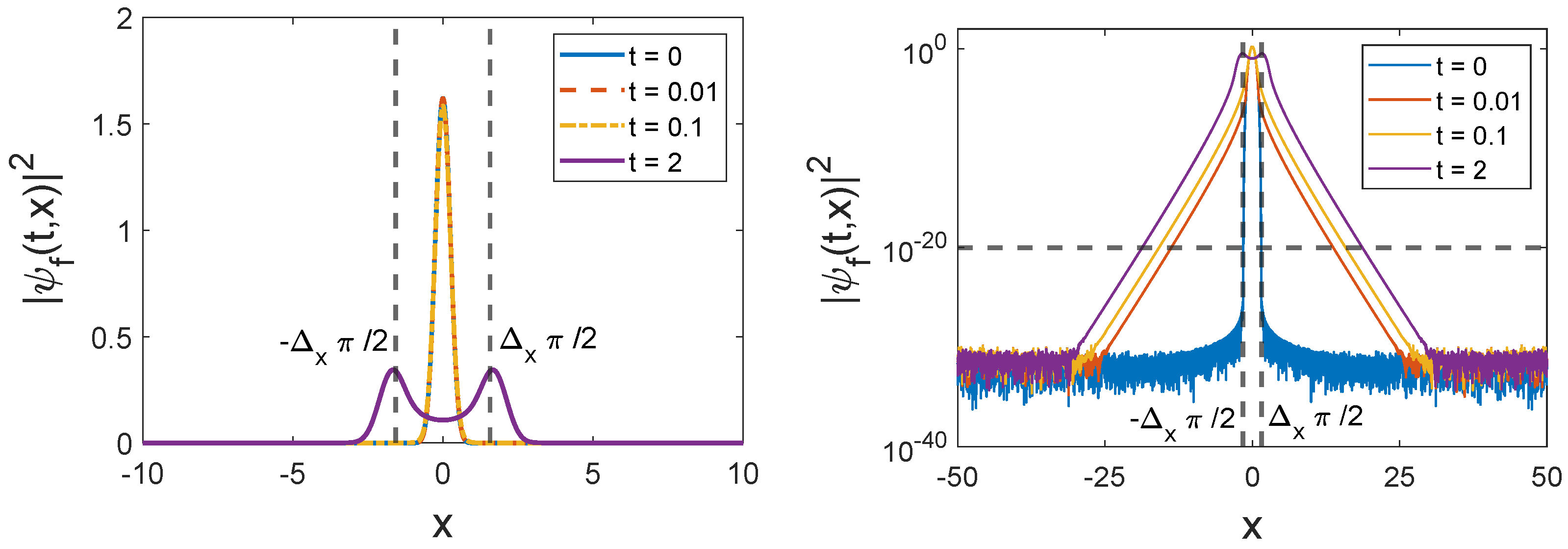
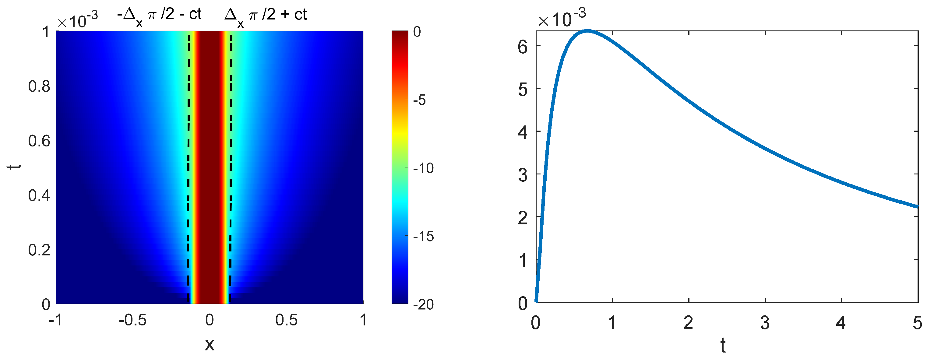
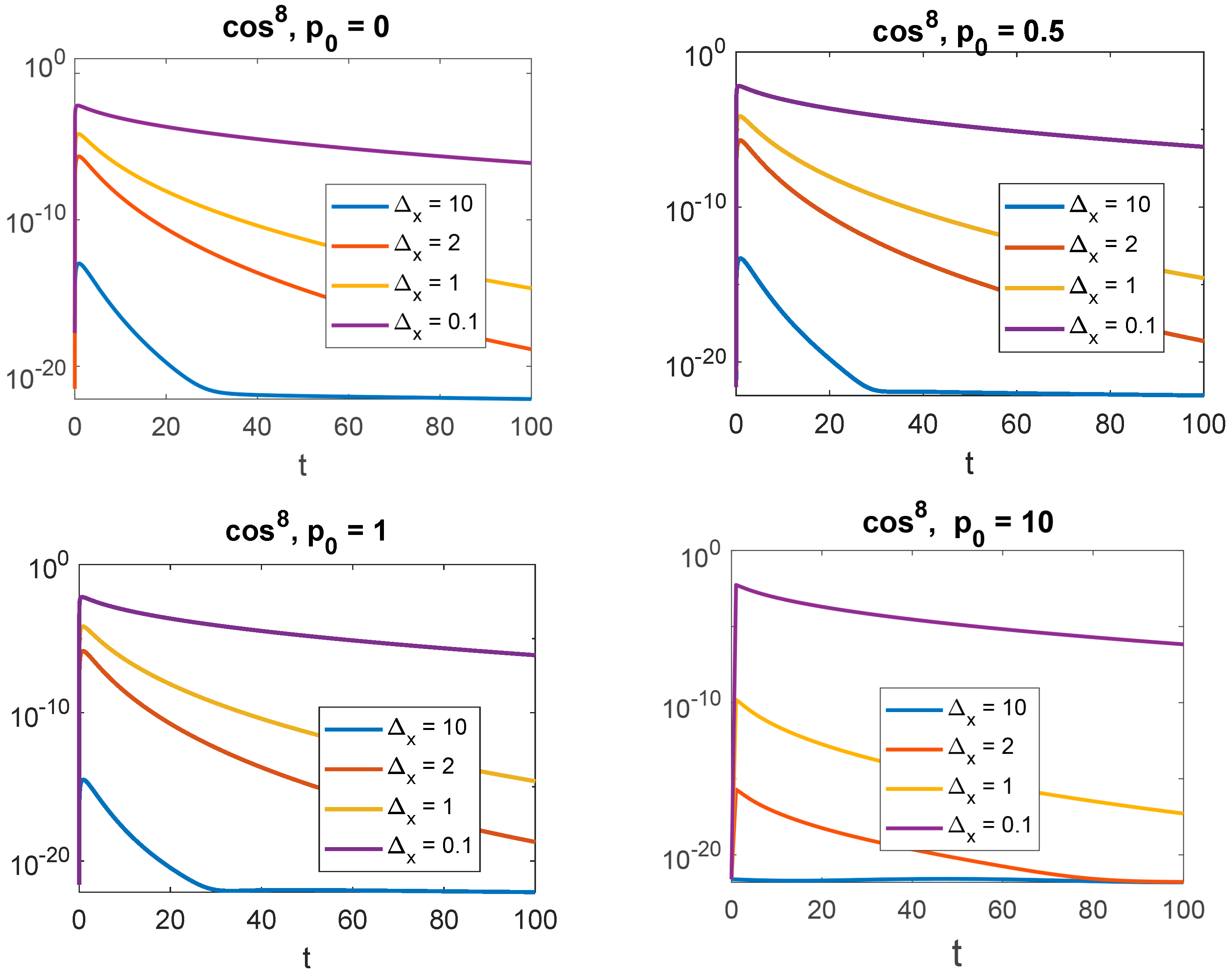
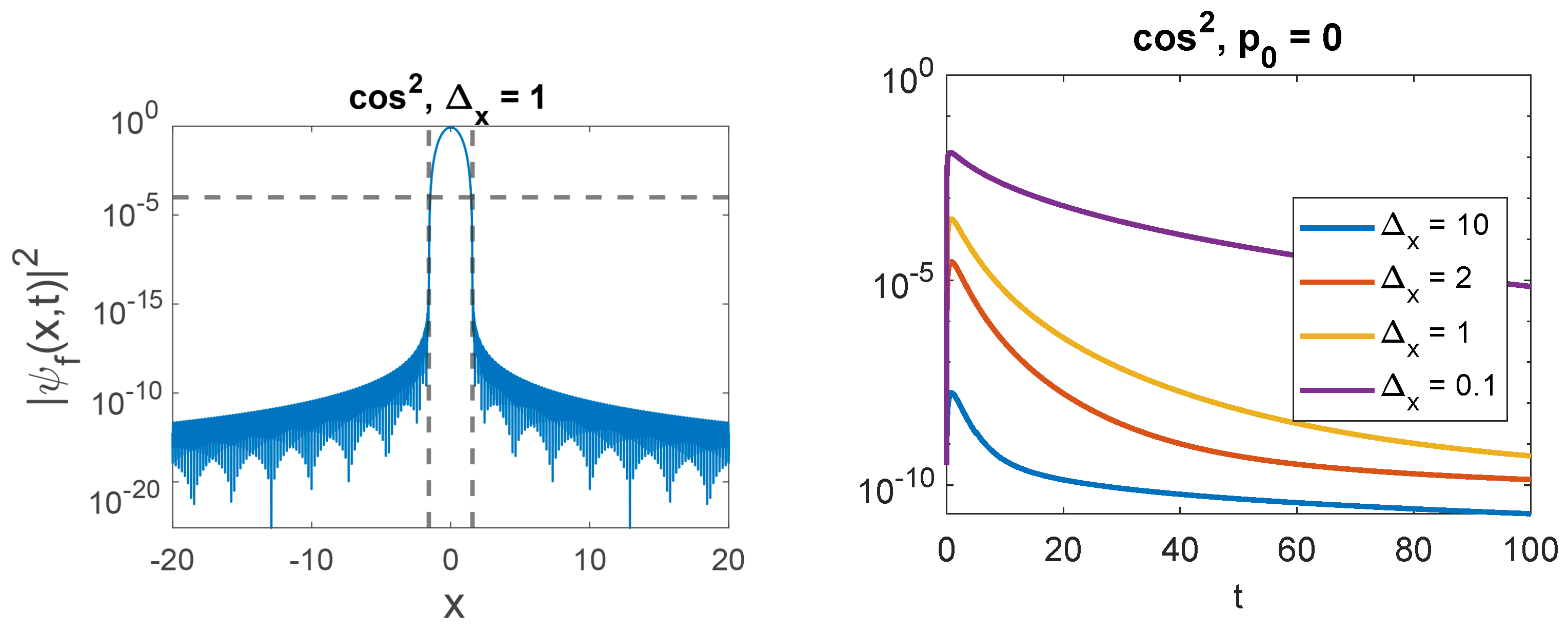
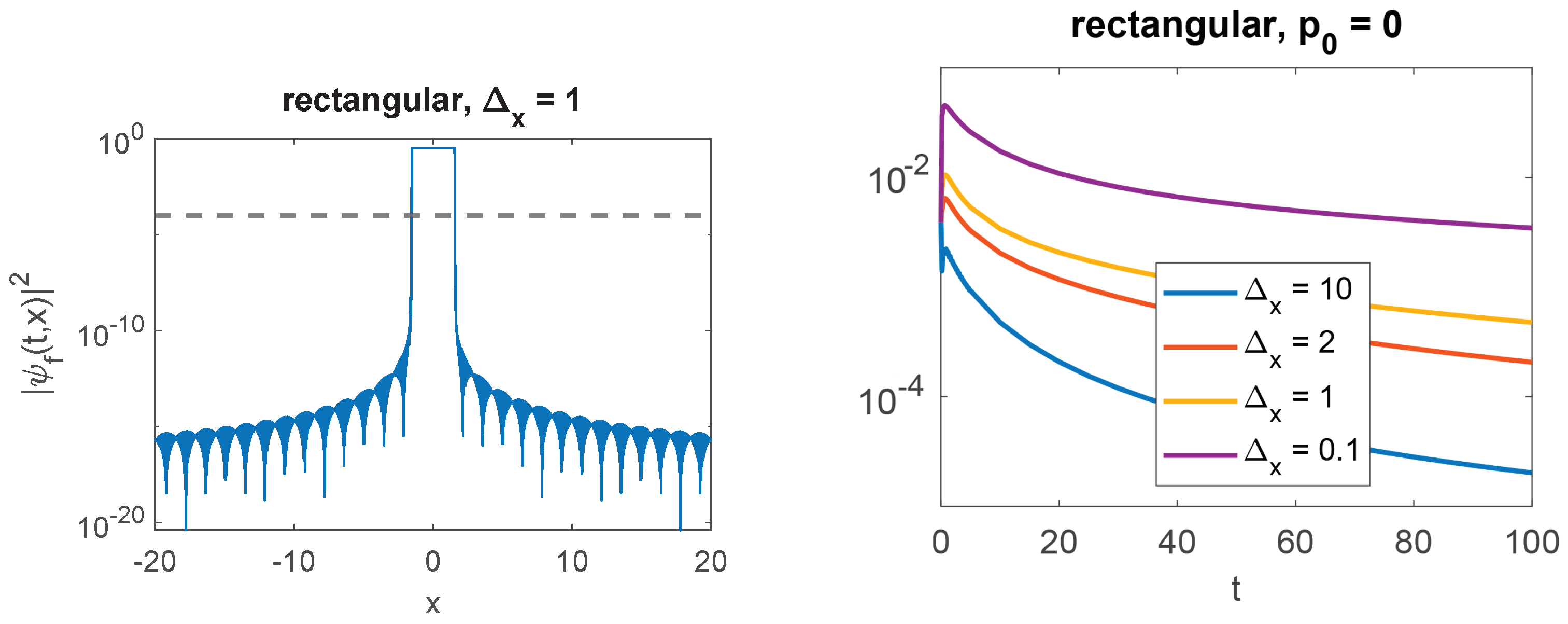
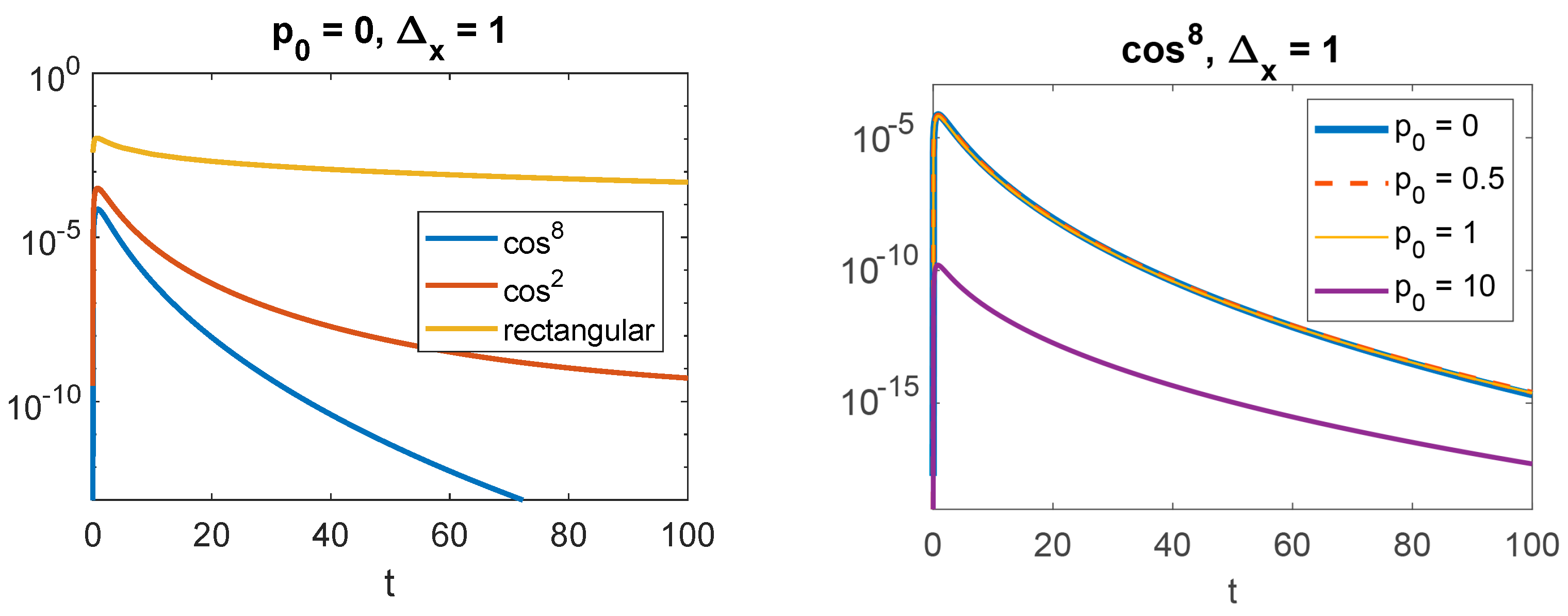
The Salpeter equation, although it is attractive as it results from quantizing the classical relativistic Hamiltonian, is usually regarded as an approximate model for a spinless particle, correctly described by the Klein–Gordon equation. Note, however, that for a neutral particle, the solutions of the Klein–Gordon equation are real and can be combined to obtain a complex wavefunction obeying the Salpeter equation [25,26].

The situation is more involved from the point of view of the FW representation. The interpretational difficulties of the standard KG or Dirac densities are related to the problems of defining a position operator. The position operator $\widehat{X}$ in the FW representation is equivalent to the Newton-Wigner position operator [23] in the standard representation. On this basis, it is often argued that the FW density is the physical one [27]. The problem is then knowing how to cope with the non-causal nature of the propagation.

The answer that has been given is, in a nutshell, that non-causality is in practice undetectable. First, it has been argued that the probability of such a detection is so low that it would be unlikely to detect such an event even over billions of years [9]. Second, it is difficult to imagine how signals could be sent superluminally since modulations cannot be produced from the exponentially decaying tail [8]. It can also be remarked that since non-causality is non-negligible only on distances of the order of a Compton wavelength (${\lambda }_c=\hslash /mc$) away from the light cone, a detection on this scale is hardly feasible for elementary particles and totally impossible for larger (not to mention macroscopic) bodies, for which the Compton wavelength falls below the Planck length. The first step in assessing whether these observations are plausible is to quantitatively compute the fraction of the wavepacket that is propagated beyond the light cone.

4. Results

4.1. Method

The initial wave packet (WP) is defined by Equation (9), which we rewrite here as

$$\psi (0,x)=\frac{1}{\sqrt{2\pi \hslash }}\int dp{e}^{ipx/\hslash }C(p;x_0,p_0)$$

(18)

where $x_0$ and $p_0$ are the average position and momentum, respectively, of our initial wave packet. We require $\psi (0,x)$ to have compact spatial support. In this work, we will set $x_0=0$ and consider three different initial WP of the form

$${\psi }_f(0,x)=(\theta (\pi {\Delta }_x/2-x)-\theta (x-\pi {\Delta }_x/2))e^{-i{p}_{0}x}f\left(x\right)$$

(19)

with $f\left(x\right)$ given by ${cos}^8(x/{\Delta }_x)$, ${cos}^2(x/{\Delta }_x)$, or 1 (yielding a rectangular distribution). ${\Delta }_x$ gives the scale of the spatial width of the packet, and $\theta \left(x\right)$ is the unit step function. $\psi (0,x)$ is normalized to 1.

The initial momentum distribution is computed as the Fourier transform of the compact wave function in coordinate space

$$C_f(p;x_0,p_0)=\frac{1}{\sqrt{2\pi \hslash }}{\int }_{-{\Delta }_x\pi /2}^{{\Delta }_x\pi /2}{\psi }_f(0,x)e^{-ipx}dx$$

(20)

hence, with the present notation, the time evolved wavefunction is given by

$$\begin{array}{cc}\hfill {\psi }_f(t,x)& =\int d{x}^{\prime }{K}^S(t,t^{\prime };x,x^{\prime }){\psi }_f(0,x^{\prime })\hfill \end{array}$$

(21)

$$\begin{array}{cc}\hfill & =\frac{1}{\sqrt{2\pi \hslash }}\int dp{e}^{ipx/\hslash }{e}^{-i{E}_{p}t/\hslash }{C}_f(p;x_0,p_0).\hfill \end{array}$$

(22)

The initial momentum space wavefunctions $C_f(p;x_0,p_0)$ can be obtained analytically,

$$C_{co{s}^m}(p;x_0,p_0)=(2m!/{\Delta }_x^m)\frac{sin\left[\left(p-p_0\right){\Delta }_x\pi /2\right]exp\left[i\left(p-p_0\right)x_0\right]}{(p-p_0){\prod }_{n=1}^{n=m/2}(p-p_0-\frac{2n}{{\Delta }_x})(p-p_0+\frac{2n}{{\Delta }_x})},$$

(23)

when the initial state is a cosine function, and

$$C_1(p;x_0,p_0)=\frac{2sin[(p-p_0){\Delta }_x\pi /2]}{p-p_0}{e}^{i\left(p-p_0\right)x_0}$$

(24)

for the case of the rectangular distribution for which $f\left(x\right)=1$. Note that the simple poles appearing in the denominator are cancelled out by the sine in the numerator.

In practice, Equation (21) is obtained numerically employing the trapezoidal method in Matlab, with the bounds on the integration variable, $p_i$ and $p_f$, taken large enough so that $C(p_{i,f};x_0,p_0)\sim 0$. Numerically, the actual computed value of the wave packet will not be exactly zero outside its compact support (including at $t=0$), but a very small number that should be smaller than our numerical zero, see Figure 1 for the $f\left(x\right)={cos}^8(x/{\Delta }_x)$ case for which the numerical zero is set at ${10}^{-20}$. The calculations based on the method employed here have recently been compared [28,29,30] to direct solutions of the relativistic wave equations obtained by employing a high-precision finite-difference scheme, resulting in an excellent agreement. In this section, all our results will be given in natural units, $\hslash =c=m=1,$; hence, the Compton wavelength is ${\lambda }_C=\hslash /mc=1$.

4.2. Numerical Results

The left panel of Figure 1 shows the probability density for a typical initial wavefunction with compact support (${\psi }_f(0,x)$ is given by Equation (19) with $f\left(x\right)={cos}^8(x/{\mathrm{\Delta }}_x)$), along with a few snapshots as the wavefunction evolves. On this scale, the tails propagating outside the light cone are not visible, so we have plotted on the right panel the same quantities on a logarithmic scale, clearly displaying beyond the light-cone propagation (the light cone position is $\pm \left(\pi /2+t\right)$ in these units). Figure 2 (left) shows a density plot for the same initial wavefunction, while the right panel shows the fraction of the density lying outside the light cone as time evolves. This fraction reaches a maximum a very short time after initial propagation and then decreases to zero for longer times. Figure 3 shows the fraction of the probability density outside the light cone for the same ${\psi }_f(0,x)$ but with different initial widths ${\Delta }_x$ and initial momenta $p_0$.

Figure 4 and Figure 5 display similar results but for an initial wavefunction ${\psi }_f(0,x)$ with $f\left(x\right)={cos}^2(x/{\Delta }_x)$ and $f\left(x\right)=1$, respectively, (only the case with initial average momentum $p_0=0$ is shown). Note that we have taken a higher value for the numerical 0, given that the momentum range over which we need to integrate in Equation (21), for each value of t, is significantly more extended than with a ${cos}^8(x/{\Delta }_x)$ function. Finally, Figure 6 compares the probability density propagating beyond the light cone for the three functions $f\left(x\right)$ we have considered in this paper (with the same initial compact support and mean momentum).

We have, in addition, included two tables.

Table 1. Time for which the fraction of the probability density propagating beyond the light cone remains above ${10}^{-4}$, for different initial wavefunctions.

	${\mathbf{\Delta }}_{\mathit{x}}=10$	${\mathbf{\Delta }}_{\mathit{x}}=2$	${\mathbf{\Delta }}_{\mathit{x}}=1$	${\mathbf{\Delta }}_{\mathit{x}}=0.1$
$co{s}^8$, $p_0=0$	-	-	-	$t\sim 27$
$co{s}^2$, $p_0=0$	-	-	$t\sim 3.1$	$t\sim 43.5$
rectangular, $p_0=0$	$t\sim 225$	$t\sim 1150$	$t\sim 2250$	$t\sim 9000$

specifies the duration of significant superluminal propagation depending on $f\left(x\right)$ (the compact support) and the width. We see that in the rectangular case for a narrow wavepacket, a fraction ($0.01$%) of the probability density remains outside the light cone for times up to $t\approx {10}^4$ in natural units (for an electron this corresponds to $1.3\times {10}^{-17}$ s).

Table 2. Time for which the fraction of the probability density lying outside the light cone is maximal, along with the corresponding value of that fraction, for different initial wavefunctions (all with $p_0=0$).

Wavefunction	${\mathbf{\Delta }}_{\mathit{x}}=10$	${\mathbf{\Delta }}_{\mathit{x}}=2$	${\mathbf{\Delta }}_{\mathit{x}}=1$	${\mathbf{\Delta }}_{\mathit{x}}=0.1$
$co{s}^8$	$t\sim 0.96$	$t\sim 0.89$	$t\sim 0.84$	$t\sim 0.65$
	$1.1\times {10}^{-13}$	$2.15\times {10}^{-6}$	$7.25\times {10}^{-5}$	$1.38\times {10}^{-3}$
$co{s}^2$	$t\sim 0.84$	$t\sim 0.84$	$t\sim 0.80$	$t\sim 0.66$
	$2.23\times {10}^{-8}$	$2.88\times {10}^{-5}$	$3.14\times {10}^{-4}$	$1.87\times {10}^{-3}$
rectangular	$t\sim 0.64$	$t\sim 0.68$	$t\sim 0.66$	$t\sim 0.63$
	$2.28\times {10}^{-3}$	$6.46\times {10}^{-3}$	$1.06\times {10}^{-2}$	$4.40\times {10}^{-2}$

, on the other hand, is interested in short times, reporting the time at which the fraction of the probability density lying outside the light cone is maximal, as well as the value of that fraction.

5. Discussion and Conclusions

As expected from mathematical arguments, our calculations confirm that the wavefunction propagates beyond the light cone as soon as $t>0$. Typical wavepackets will have a spatial distribution ${\Delta }_x$ much larger than the Compton wavelength ${\lambda }_C$. In this case, the propagation beyond the light cone appears as a small transient effect, though not totally negligible at short times (see the ${\Delta }_x=10$ curve in Figure 5). Note that short times, of the order of $t\approx 1$ in the units used here, would lie for an electron in the zeptosecond regime, a regime that is near experimental reach [31]. Of course for heavier particles, the time scale scales inversely to the mass, so that for macroscopic bodies $t\approx 1$ would be shorter than the Planck time.

Even at considerably longer times, there is still a non-negligible probability outside the light cone (see Table 1)). For narrower wavepackets, the fraction of the probability distribution beyond the light cone can reach a non-negligible percentage (see the ${\Delta }_x=0.1$ curve in Figure 3, Figure 4 and Figure 5). While it is generally believed that the single particle formalism breaks down for wavepackets narrower than ${\lambda }_C$ (but see [32,33,34]), the propagating wavepacket would still contribute to the one-particle sector of the corresponding quantum-field theoretical description [8,17]. This does not necessarily entail that the superluminal propagation could actually be detected, but, to the extent that the spatial density defined above is the correct physical one, our results indicate this possibility must be kept open.

Another interesting effect is the role of the initial average momentum. From Figure 3, one can see that the fraction of the probability density leaking beyond the light-cone decreases as $p_0$ increases. Somewhat paradoxically, wavepackets in the ultrarelativistic regime ($p_0\sim 10$) remain almost entirely within the light cone, while wavepackets with initial zero momentum (whose average position does not move) are those that display the highest proportion of superluminal propagation (see Figure 6). It would be interesting to understand the reasons for this behavior. The role of the shape of the wavepacket, which determines the range of the contributing momenta in Equation (21), is also interesting. From our choices for $f\left(x\right)$, we can say that beyond the light cone, spreading increases as the momentum range increases. Here too, there is no obvious argument to explain this behavior.

In summary, motivated by the issue of the physicality of the Foldy–Wouthuysen (FW) density, we have numerically explored the time evolution of free relativistic wavefunctions propagated by the sole positive energy propagator. We have done so by choosing three different initial wavefunctions with compact support and varying parameters. We conclude from our findings that beyond the light cone, propagation is a very small effect that is non-negligible for particles having a small mass (of the order of elementary particles) over a short time after preparation of the initial state. It is, however, impossible to assert that this effect cannot lead to any observational consequences if the FW density is taken as being the physically meaningful quantity.

References

1. Hegerfeldt, G.C. Instantaneous spreading and Einstein causality in quantum theory. Ann. Phys. 1998, 7, 716–725. [Google Scholar] [CrossRef]
2. Kosinski, P. Salpeter Equation and Causality. Prog. Theor. Phys. 2012, 128, 59–65. [Google Scholar] [CrossRef]
3. Beck, C. Local Quantum Measurement and Relativity; Springer Nature Switzerland: Cham, Switzerland, 2021. [Google Scholar]
4. Greiner, W. Field Quantization; Springer: Berlin/Heidelberg, Germany, 1996. [Google Scholar]
5. Padmanabhan, T. Obtaining the non-relativistic quantum mechanics from quantum field theory: Issues, folklores and facts. Eur. Phys. J. C 2018, 78, 563. [Google Scholar] [CrossRef]
6. Kowalski, K.; Rembielinski, J. Salpeter equation and probability current in the relativistic Hamiltonian quantum mechanics. Phys. Rev. A 2011, 84, 012108. [Google Scholar] [CrossRef]
7. Zou, L.; Zhang, P.; Silenko, A.J. Position and spin in relativistic quantum mechanics. Phys. Rev. A 2020, 101, 032117. [Google Scholar] [CrossRef]
8. Pavsic, M. Localized States in Quantum Field Theory. Adv. Appl. Clifford Algebr. 2018, 28, 89. [Google Scholar] [CrossRef]
9. Ruijsenaars, S.N.M. On Newton-Wigner localization and superluminal propagation speeds. Ann. Phys. 1981, 137, 33–43. [Google Scholar] [CrossRef]
10. Rosenstein, B.; Usher, M. Explicit illustration of causality violation: Noncausal relativistic wave-packet evolution. Phys. Rev. D 1987, 36, 2381. [Google Scholar] [CrossRef]
11. Al-Hashimi, M.H.; Wiese, U.J. Minimal position-velocity uncertainty wave packets in relativistic and non-relativistic quantum mechanics. Ann. Phys. 2009, 324, 2599–2621. [Google Scholar] [CrossRef]
12. Eckstein, M.; Miller, T. Causal evolution of wave packets. Phys. Rev. A 2017, 95, 032106. [Google Scholar] [CrossRef]
13. Torre, A.; Lattanzi, A.; Levi, D. Time-Dependent Free-Particle Salpeter Equation: Numerical and Asymptotic Analysis in the Light of the Fundamental Solution. Ann. Der Phys. 2017, 529, 1600231. [Google Scholar] [CrossRef]
14. Greiner, W. Relativistic Quantum Mechanics; Springer: Berlin/Heidelberg, Germany, 1996. [Google Scholar]
15. Wachter, A. Relativistic Quantum Mechanics; Springer: Berlin/Heidelberg, Germany, 2011. [Google Scholar]
16. Salpeter, E.E. Mass Corrections to the Fine Structure of Hydrogen-Like Atoms. Phys. Rev. 1952, 87, 328. [Google Scholar] [CrossRef]
17. Rosenstein, B.; Horwitz, L.P. Probability current versus charge current of a relativistic particle. J. Phys. A Math. Gen. 1985, 18, 2115. [Google Scholar] [CrossRef]
18. Lucha, W.; Schoeberl, F.F. All Around the Spinless Salpeter Equation. arXiv 1994, arXiv:hep-ph/9410221. [Google Scholar]
19. Foldy, L.L.; Wouthuysen, S.A. On the Dirac Theory of Spin 1/2 Particles and Its Non-Relativistic Limit. Phys. Rev. 1950, 78, 29. [Google Scholar] [CrossRef]
20. Case, K.M. Some Generalizations of the Foldy–Wouthuysen Transformation. Phys. Rev. 1954, 95, 1323. [Google Scholar] [CrossRef]
21. Alkhateeb, M.; Matzkin, A. Relativistic Bohmian Trajectories and Klein–Gordon Currents for Spin-0 Particles. Found. Phys. 2022, 52, 104. [Google Scholar] [CrossRef]
22. Redmount, I.H.; Suen, W.M. Path integration in relativistic quantum mechanics. Int. J. Mod. Phys. A 1993, 8, 1629–1635. [Google Scholar] [CrossRef]
23. Newton, T.D.; Wigner, E.P. Localized States for Elementary Systems. Rev. Mod. Phys. 1949, 21, 400. [Google Scholar] [CrossRef]
24. Karpov, E.; Ordonez, G.; Petrosky, T.; Prigogine, I.; Pronko, G. Causality, delocalization, and positivity of energy. Phys. Rev. A 2000, 62, 012103. [Google Scholar] [CrossRef]
25. Pavsic, M. Manifestly covariant canonical quantization of the scalar field and particle localization. Mod. Phys. Lett. A 2018, 33, 1850114. [Google Scholar] [CrossRef]
26. Pavsic, M. A new perspective on quantum field theory revealing possible existence of another kind of fermions forming dark matter. Int. J. Geom. Meth. Mod. Phys. 2022, 19, 2250184. [Google Scholar] [CrossRef]
27. Silenko, A.J.; Zhang, P.; Zou, L. Reply to Comment on “Relativistic Quantum Dynamics of Twisted Electron Beams in Arbitrary Electric and Magnetic Fields”. Phys. Rev. Lett. 2019, 122, 159302. [Google Scholar] [CrossRef] [PubMed]
28. Gutiérrez de la Cal, X.; Alkhateeb, M.; Pons, M.; Matzkin, A.; Sokolovski, D. Klein paradox for bosons, wave packets and negative tunnelling times. Sci. Rep. 2020, 10, 19225. [Google Scholar] [CrossRef] [PubMed]
29. Alkhateeb, M.; Gutierrez de la Cal, X.; Pons, M.; Sokolovski, D.; Matzkin, A. Relativistic time-dependent quantum dynamics across supercritical barriers for Klein–Gordon and Dirac particles. Phys. Rev. A 2021, 103, 042203. [Google Scholar] [CrossRef]
30. Alkhateeb, M.; Matzkin, A. Relativistic spin-0 particle in a box: Bound states, wave packets, and the disappearance of the Klein paradox. Am. J. Phys. 2022, 90, 297. [Google Scholar] [CrossRef]
31. Mourou, G.; Mironov, S.; Khazanov, E.; Sergeev, A. Single cycle thin film compressor opening the door to Zeptosecond-Exawatt physics. Eur. Phys. J. Spec. Top. 2014, 223, 1181. [Google Scholar] [CrossRef]
32. Bakke, F.; Wergeland, H. Wave packets of relativistic electrons. Physica 1973, 69, 5–11. [Google Scholar] [CrossRef]
33. Hoffmann, S.E. The minimum width in relativistic quantum mechanics. J. Phys. B 2018, 51, 165302. [Google Scholar] [CrossRef]
34. Krekora, P.; Su, Q.; Grobe, R. Relativistic Electron Localization and the Lack of Zitterbewegung. Phys. Rev. Lett. 2004, 93, 043004. [Google Scholar] [CrossRef]
Figure 1. ψ f ( t , x ) 2 for the function with compact support f ( x ) = cos 8 ( x / Δ x ) (with Δ x = 1 and p 0 = 0 ) is shown for different values of t (in natural units = c = m = 1 ). Left panel displays the plots in the usual (linear) scale and the right panel shows the same quantities with a logarihtmic scale. The horizontal dashed line indicates the numerical zero. The initial wavefunction has compact support (no density above the numerical zero), whereas beyond the light-cone propagation appears for times t > 0 .
Dynamics 03 00005 g001
Figure 2. Left panel: time evolution of log [ ψ f ( t , x ) 2 ] for the function with initial compact support f ( x ) = cos 8 ( x / Δ x ) (with Δ x = 1 and p 0 = 0 ) for short values of t. Note that the tails propagating beyond the light cone appear as soon as t > 0 . Right panel: Fraction of that same wave packet outside the light cone, where the transient aspect can be noticed.
Dynamics 03 00005 g002
Figure 3. Fraction of the probability density lying outside the light cone for an initial wavepacket ψ ( 0 , x ) [Equation (19)] with f ( x ) = cos 8 x / Δ x , where Δ x and p 0 vary as indicated.
Dynamics 03 00005 g003
Figure 4. Left panel: ψ f ( t = 0 , x ) 2 is plotted in logarithmic scale for the function with compact support f ( x ) = cos 2 ( x / Δ x ) (with Δ x = 1 and p 0 = 0 ). Right panel: fraction of the probability density leaking outside the light cone as this initial wavepacket evolves (each curve shows the result for a different width Δ x ).
Dynamics 03 00005 g004
Figure 5. Same as Figure 4 but for an initial rectangle distribution, f ( x ) = 1 .
Dynamics 03 00005 g005
Figure 6. Fraction of the probability density leaking outside the light cone as time evolves. Left panel: Comparison of the three wave different initial compact supports f ( x ) considered in this work, see Equation (19), with p 0 = 0 and Δ x = 1 . Right panel, for the case f ( x ) = cos 8 ( x / Δ x ) , comparison of different values of the initial momentum p 0 (with Δ x = 1 in all cases).
Dynamics 03 00005 g006