Article

Complex Network Methods for Plastic Deformation Dynamics in Metals

1
Department of Materials Engineering, Ben-Gurion University of the Negev, Beer Sheva 8410501, Israel
2
Department of Innovative Technologies and Methods of Teaching Natural Sciences, South Ukrainian National Pedagogical University Named after K.D. Ushinsky, 65020 Odesa, Ukraine
3
Department of Computer Science and Applied Mathematics, Kryvyi Rih State Pedagogical University, 50086 Kryvyi Rih, Ukraine
4
Department of Biology and Chemistry, Drohobych Ivan Franko State Pedagogical University, 82100 Drohobych, Ukraine
*
Author to whom correspondence should be addressed.
Dynamics 2023, 3(1), 34-59; https://doi.org/10.3390/dynamics3010004
Submission received: 27 September 2022 / Revised: 20 January 2023 / Accepted: 22 January 2023 / Published: 30 January 2023

Abstract

:
Plastic deformation of DC04 steel is regarded as a nonlinear, complex, irreversible, and self-organized process. The stress–strain time series analysis provided the possibility to identify areas of (quasi-)elastic deformation, plastic deformation, and necking. The latter two regions are the most informative. The area of inelastic deformation is reflected by collective, self-organized processes that lead to the formation of pores, and finally, the development of microcracks and a general crack as the cause of sample failure. Network measures for the quantitative assessment of the structural deformations in metals are proposed. Both spectral and topological measures of network complexity were found to be especially informative. According to our results, they can be used not only to classify the stages of plastic deformation, but also, they can be applied as a precursor of the material destruction process.

1. Introduction

A challenging frontier in physics concerns the study of complex systems. In 2000, Stephen Hawking, in response to a question about the way that science is developing, replied: “I think the next century will be the century of complexity”. He was pointing towards the increasing importance of a set of scientific ideas that emerged at the beginning of 1980s that allow us to find order within highly complex, interconnected systems, such as the weather, traffic movement, the stock market, and the ecosystem [1,2]. One of the creators of the modern theory of complex networks, referring to the analysis of Web of Science data for more than 100 years, demonstrated the rapid growth and increase in multidisciplinary physics—a century of physics [3,4]. Combining these practically realizable forecasts today, we can assume that the current century is the century of the physics of complex systems.
Complexity and quantitative measures of complexity have long been of interest to researchers. Many fundamental results in this area were obtained in the works of A. Kolmogorov [5], P. Anderson [6], I. Prigogine [7], M. Hell-Mann [8], and G. Parisi [9]. The most crucial characteristics of complex systems are listed in the definitions of complexity that are now in use: nonlinearity, feedback, spontaneous order, robustness and lack of centralized control, emergence, hierarchical organization, and numerosity. These characteristics distinguish complex systems from other simple systems, but they are neither required nor sufficient for a system to be classified as a complex system [10]. Complex systems are made up of several microscopic parts that interact with one another in complicated ways. Many real-world systems can be viewed as complex systems where the interactions between the pieces, rather than the individual parts, contain crucially significant information. Complex systems are characterized by specific time-dependent interactions among their many constituents. As a consequence, they often manifest rich, nontrivial and unexpected behavior [3].
There are significant challenges in formal modeling and simulation of complex systems [11]. A network paradigm can be used to depict a complex system because it typically consists of numerous components and their interactions, and these components can be presented as nodes and interactions between them as links [12]. Real-world systems can be greatly simplified by complex networks, which can also maintain the crucial details of the interaction structure that underlies complex emergent phenomena. This makes the complex network an excellent tool for studying complex systems [13,14].
Particularly successful was the approach associated with the use of complex network methods to characterize dynamic systems based on time series [15,16]. Although nonlinear time series analysis and complex network theory are both widely regarded as well-established fields of complex systems sciences closely related to nonlinear dynamics and statistical physics, the combination of the two approaches has emerged as an active area of nonlinear time series analysis and has produced fundamental findings regarding the structural organization of nonlinear dynamics as well as successfully addressing numerous applications from a wide range of fields [17,18]. New fundamental ideas of the complex network theory approaches allow obtaining new results not only in the field of nonlinear analysis of time series, but also in traditionally physical areas of science and applications: percolation on networks [19], critical phenomena, phase transitions, coevolution [20], etc.
Although over the past decade networks have become the paradigm for modeling complex systems, nevertheless, as simple collections of nodes and connections, they are inherently limited by pairwise interactions, which in turn limits our ability to describe, understand, and predict complex phenomena resulting from interactions of a higher order. Therefore, a new framework for modeling higher-order systems has recently been proposed, where hypergraphs and simplicial complexes are used to describe complex interaction models between any number of agents [21,22].
One of the fundamental problems of physical materials science is the explanation of the complex regularities observed in the experiment for the emergence and development of defect structures that form during the plastic deformation of a material. A deformable material is a complex dynamic system in which, under the influence of an external load, the material is transferred to a state far from thermodynamic equilibrium. This leads to the development of dissipative instabilities in the system, leading to the formation of various types of inhomogeneous defect structures, including dislocation structures. Plastic deformation of metals is spatially inhomogeneous and discontinuous in time due to the discrete nature of plasticity carriers−lattice dislocations [23]. The discreteness of dislocation processes is the root cause of local fluctuations in stresses and strains. However, a typical stress–strain curve taken with the accuracy of modern equipment turns out to be smooth. The reason for this is that the global stress–strain curve is the result of averaging over the deformed volume and time, and as such does not reveal the discontinuity of plastic flow.

2. Analysis of Previous Studies

Network science is an extensive, interdisciplinary research area that covers many other disciplines—computer science, mathematics, social sciences, and, especially, physics. For the last several decades, many studies have been devoted to the granular materials in which the evolution of discrete, macroscopic particles leading to many interesting consequences give interesting insights. Further obtained results and conclusions find their applicability for other heterogeneous materials and the analysis of their response to different external perturbations.
Paradopolulos et al. [24] devoted a review study on the network-based approaches for studying heterogeneous architectures of granular materials across different temporal and time scales in complex systems. They studied the diverse set of network-based approaches that could give new insights about their underlying physics. They also outlined a few open questions and highlighted especially promising directions in the analysis of granular materials and their networks.
In the next paper [25], the authors extended graph-theoretic approaches by utilizing multilayer networks for quantification of the progression of mesoscale structure in compressed granular materials. Considering particles of a quasi-two-dimensional aggregate of photoelastic disks as nodes of a network and the interconnections between them as edges, they constructed a multilayer system of linked static forces that existed at each strain step. By using the generalization of the community detection method, researchers extracted the inherent mesoscale structure from the system. Both normal and tangential forces were considered, and it was found that those forces displayed different progression throughout compression. They also found that the considered approach was able to distinguish a subsystem of low-friction particles within a bath of higher friction particles by using the multilayer network of tangential forces. Thus, it can be seen that multilayer networks represent significant prospects for the classification and comparison of systems under different external conditions.
Giusti et al. [26] demonstrated the utility of a trio of related but fundamentally distinct measurements of the mesoscale structure of force chains in two-dimensional packings and statistics derived with the usage of tools from algebraic topology which, in combination, provided a toolset for the analysis of force chain architecture with pressure. The described methods could be generalized to three-dimensional packings and the analysis of the deformations of packings under stress or strain.
Walker et al. [27] analyzed the time series of a proxy for granular friction of photoelastic disks sheared by a rough slider pulled along the surface with the usage of complex systems methods. Nonlinear surrogate time series methods presented that the stick-slip behavior was much more complex than a periodic dynamic description. Using the phase space reconstruction method, they presented that the dynamics could be locally captured within 4–6 dimensional subspaces. Also, the phase space networks of the slider time series, constructed by connecting nearby phase space points, were tested. This technique provides interesting perspectives for capturing key features of the dynamics.
In this study [28], a random graph process was used to model the formation of a molecular network from multifunctional precursors. Their approach did not account for the spatial position of the monomers explicitly. However, they derived Euclidian distances between monomers from their topological information. According to their conclusions, the model can be applied to large time scales. The model can predict the phenomena of structural inhomogeneity, gelation, microgelation, and conversion-dependent reaction rates. The analysis of the size distribution, crosslink distance, and gel-point conversion is derived from the resulting nonhomogeneous network. Moreover, authors used new community descriptors for the molecular simulation that could be especially useful when explaining the evolution of the gel as being a single molecule.
Tordesillas et al. [29] devoted their study to the complex network approaches for analyzing X-ray micro-CT measurements of grain kinematics in Hostun sand under triaxial compression. They found that the network nodes with the least mean shortest path length or highest relative closeness centrality resided in the region where the persistent shear band ultimately developed. The network communities’ borders that reflected the shear band’s boundaries and thickness provided corroborating evidence of early detection of strain localization. Their results provide higher possibility of early-stage identification of the formation and the location of the persistent shear band, well before peak shear stress. The robustness of the results was confirmed by the grain-scale digital image correlation strain measurements and statistical tests.
Karapiperis and Andrade [30] revealed the interplay between the topological, kinematic, and force signature of the processes of self-organization in dry granular systems. They identified communities of similar topology, kinematics, and kinetics of those processes using Level-Set Discrete Element simulations of an in situ triaxial compression experiment and complex network methods.
Zhang et al. [31] proposed a new feature extraction model of vibration signals for bearing fault diagnosis based on the approach that allows to reconstruct a network of a particular system from its time series (visibility graph). They extracted 15 visibility graph features from the binary matrix using the toolkit of the complex network theory and image processing methods. The visibility graph model presented the highest accuracy score compared to other models presented in the study. Inspired by the visibility graph method, Mohebian et al. [32] proposed a new meta-heuristic optimization algorithm for identifying structural damage, called visible particle series search. Their results demonstrated high accuracy, reliability, and computational efficiency of the proposed algorithm.
Walker et al. [33] studied plastic deformation in a plain strain compression test of a dense sand specimen using functional networks. Using digital image correlation, they obtained kinematic information for the deforming material. Also, by applying two types of complex network with different connectivity rules establishing links between the network nodes, those images were summarized. Each network provided useful information about plastic deformation and nonaffine kinematical processes emerging within the material.
Meng and Terentjev [34] theoretically investigated the mechanical response of a transient network, which was characterized by dynamically breaking and re-forming crosslinks, and accounted for the finite chain extensibility. They built the general theory that incorporated the widely accepted empirical model of hyper-elasticity at large deformations (the Gent model) and naturally included the microscopic behavior of transient crosslinks under the local tension applied to them.
Ghaffari and Young [35] analyzed with the functional networks the evolution of shear rupture fronts in laboratory earthquakes. They showed that the mesoscopic characteristics of functional networks carried the characteristic time for each phase of the rupture evolution. According to the applied approach, the classified rupture fronts in network states presented a clear separation into three main groups, indicating different states of rupture fronts.
Despite numerous experimental and theoretical works in the field of elastic–plastic destruction of metals, they are far from being completed. This is especially true in the field of plastic deformation, where sometimes diametrically opposite points of view are considered. For example, in the article of Zuev et al. [36], an autowave approach is proposed. Vinogradov et al. [37] proposed a dislocation model of deformation of materials. Among the fundamental theoretical studies, one can single out a paper in which the multilevel dynamics of transformations of defective structures in the process of plastic deformation is considered [38]. However, with all the fundamental and theoretical rigor, it was not possible to quantitatively describe the hierarchical picture of the processes of transformation of defective structures. Our proposed approach is a completely new look at the old problem and, as follows from the results obtained below, allows us to quantitatively separate the main phases of the deformation and destruction of metals and, in addition, to establish signals for early diagnosis of catastrophic processes of material destruction. Early identification and prediction of destructive processes during plastic deformation of metals are some of the most difficult tasks in materials science. From the presented analysis of previous works, it can be seen that although there are certain advances in this area, there is still quite a lot of work. It can be seen that the theory of complex networks has found application in various studies, but here we would like to present the possibility of constructing indicators (indicators-precursors) of the current (further) state of plastic deformation during the strain of metal.

3. Materials and Methods

We analyze the complexity of the stress–strain curve time series σ ϵ for DC04 steel with a working part length of 0.05 m, a width of 0.02 m, and a tensile rate of 0.06 m/s (see Figure 1). DC04 is a highly recommended material for interior and external vehicle parts due to its inherent benefits over other steels. When rigidity, strength, and ductility are crucial factors, it is employed in deep drawing and bending processes [39]. The σ value, as well as its combinations, such as ε / σ , ε / σ , returns of ε / σ r e t ( ε / σ ) (see Equation (1)) are subject to fluctuations, which contain important information about the dynamics of micromechanisms in the process of destruction. Empirical analysis of these time series made it possible to single out ε / σ as the most informative time series.
All of the presented measures were calculated with the sliding window approach [40,41,42,43,44,45,46,47,48,49]. In accordance with the technique, we emphasize the fragment of predetermined length in which the computation of the relevant measure is obtained. The series is then moved forward in time by a predetermined time step, and the process is repeated until all of the series’ elements have been used. We may examine changes in system complexity by comparing the estimated measure of complexity and the actual time series of the stress–strain curve. All of the presented measures are calculated with the window size w = 250 and step size h = 5 that corresponds to the separation between each window.
All of the presented measures are implemented with the Python programming language. Each measure is organized in the web-interactive computational document—Jupyter Notebook. The document is freely available at https://github.com/Butman2099/Complex-systems-measures (accessed on 27 January 2023).
When investigating complex systems using graph-based approaches, it is important for us to have both quantitative and qualitative results of our research. 
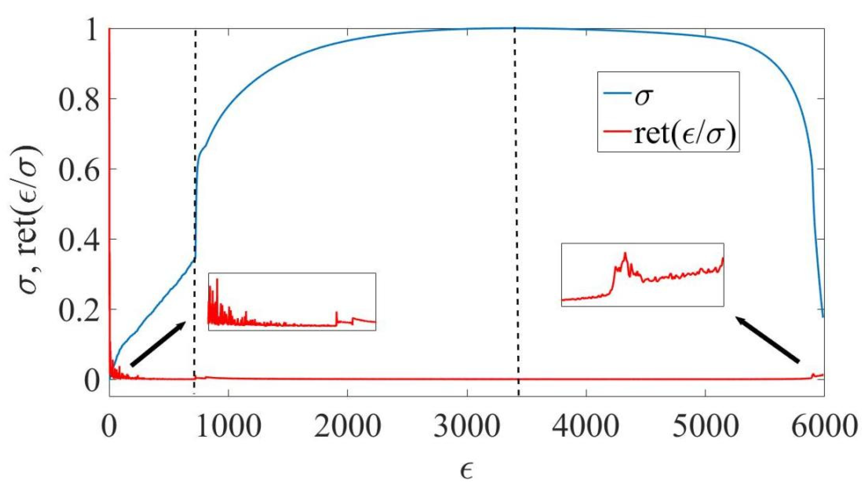
Section 5 presents not only the comparative dynamics of indicators along with the stress–strain curve, but also the “visibility relationships” of the values of the series under study based on approaches such as the visibility graph (VG) and the recurrence plot (RP) that are described later. A graph representation with the degrees of connection of each node is also presented, relying on each of the approaches. We found that the standardized “returns” of the studied series reflect the self-organized dynamics of this series (visibility connections, graph-based representation) in the most efficient way. The returns of the series can be defined as
G t = ln x t + Δ t ln x t x t + Δ t x t / x t
for t = 1 ,     ,   N 1 . Here, N is length of the initial time series, Δ t —time lag (in our case Δ t = 1 ). The standardization is expressed as g t G t G / Ω , where Ω stands for the standard deviation of G ; —average over the time period under study.
While VG does not have the dependence on any parameters for its estimation, recurrence network relies on such ones as embedding dimension d E , time delay τ , and recurrence threshold ε . When we analyze a time series of the real world, neither d E nor τ are known. One of possible approaches for obtaining desirable d E is the false nearest neighbors (FNN) method [50]. For choosing τ , we can use either the first root of the auto-correlation function (ACF) or the first minimum of the time-delayed mutual information [51]. Empirically, we have chosen d E = 3 and τ = 1.
The choice of the recurrence threshold parameter has been extensively studied in the literature [52,53,54,55]. Often, the decision of selection of the recurrence threshold depends on the data analyst himself and his understanding of the system being studied. Choosing ε 0 , will cause our network to be very sparsed. If ε 0 , the network will be highly connected. Studying the dynamics of the stress–strain curve with the sliding window procedure, we need ε to be adaptable to the structure of the studied subspace of the system. Starting the selection of ε from very large values will cause a high dense edge distribution of the network. Such a large amount of less important interconnected nodes will hide all feasible information about the studied system. The necessary information is best preserved when the threshold is sufficiently small, whereas the choice of sufficiently large ε would be effective for dealing with noise [56]. It is worth considering that the studied series is not smoothed: the transition from elastic to plastic deformation and the stage of fracture have very high rises and falls in the fluctuations of their initial values and returns. This can break the connections between different components of the series since the distance between points that characterize those stages and the points of other areas would exceed ε [57]. These unconnected components would make the shortest path length l i j = that would cause problems with the computation of some graph-based indicators.
Different studies were proposed for obtaining adequate value of ε [58,59,60]. We have simplified the procedure for choosing the threshold parameter. In this study, we are interested in selecting optimal ε that would make the whole network connected despite the studied structure of a particular fragment (window). Here, we start with the sufficiently small threshold (in this case, ε i n i t = 0.1 ). After the initialization, we increase its value by a predefined increment value Δ ε (in this case, Δ ε = 0.1 ). Increment of the recurrence threshold occurs until the graph is considered connected. The obtained value serves for further computations.

4. Network Measures of Complexity

A complex network is often represented as a graph G = V , E which consists of two sets, V and E , where V is the set of vertices (nodes or points) of G that may represent the price of a stock or, as in our case, the stress applied to the material; and E is the set of edges (links or lines) representing pairs of connected elements of V [61]. The studied vertices are indexed as i = 1 ,   ,   N , where N is the number of the vertices in G . A particular edge in a studied graph, e i j E , can be represented (identified) by pair i , j . A graph G is called undirected if i , j E j , i E . For a directed graph, the opposite relation is true. Also, a graph may contain loops, where an edge that goes from a vertex returns to itself. The connectivity of a graph can be reflected by the adjacency matrix A = A i j N × N . If vertices i and j are connected by an edge i , j , then these vertices are called adjacent and A i j = A j i = 1 . In the opposite case, A i j = A j i = 0 .

4.1. Visibility Graph Representation

The VG considers simple mapping from the time series to the network domain. For a given time series x i   |   i = 1 ,   , N , we link two vertices x i and x j by an edge i ,   j if the following condition is applied [62,63]:
x k < x j + x i x j t j t k / t j t i ,   for   t i < t k < t j .
The adjacency matrix (Aij) of the following VG can be written as
A i j = k = i + 1 j 1 H x k < x j + ( x i x j ) ( t j t k ) / ( t j t i )
where H · is the Heaviside function.
A horizontal visibility graph (HVG) provides a simplified version of the VG approach. Luque et al. [64] proposed to consider the same set of vertices as in the VG. However, the set of edges has to fulfill the horizontal visibility criterion:
x k < m i n x i ,   x j ,   for   t i < t k < t j .
The adjacency matrix (Aij) of the HVG has the following form:
A i j = k = i + 1 j 1 H x i x k H x j x k .
Since the HVG is a subgraph of the VG with the same vertex set, VG and HVG capture essentially the same properties of the system under study. However, according to the criterion described by Equation (4), the HVG possesses restrictive visibility compared to the classic VG; i.e., the set of edges associated with the HVG is a subset of the VG. Since the HVG has a smaller number of edges, it increases demand regarding the length of the studied fragment. Another difference that distinguishes the horizontal graph in comparison with the classical one is that it mostly captures short-range dependence of the system, while the visibility according to Equation (2) captures both short- and long-range correlations among the values of a series. This criterion is especially important when studying the complex, nonlinear, and self-organized dynamics of the destruction of materials. Thus, in our analysis, we will rely on the classical VG.

4.2. Recurrence Plots and Networks

Recurrence of states (trajectories) is a key characteristic of chaotic, nonlinear, and deterministic systems, where the observed trajectories after some time become arbitrarily similar to the preceding ones [65,66]. A recurrence plot (RP) is the visualization of recurrences from the set of (original or reconstructed) state vectors that represent a discrete sampling of the trajectory of the underlying system (for example, the chaotic attractor of a dissipative system) [55,67]. The recurrence matrix R ε of RP is defined as
R i j ε = H ε X i X j ,
where · can be any norm in phase space (in our case, it is a Euclidean norm). A threshold parameter ε determines whether two state vectors are close or not. By using a two-dimensional graphical representation of an RP, we may examine the recurrences of the m -dimensional phase space trajectory. Black and white dots represent recurrent and non-recurrent pairs of vectors, respectively.
Reinterpreting the mathematical structure of R ε as the adjacency matrix A of an adjoint complex network embedded in phase space is a critical component of the recurrence network technique. The recurrence adjacency matrix can be presented as
A ε = R ε I ,
where I is the identity matrix. The complex network defined this way is called ε-recurrence network (RN). Since R ε represents the recurrence states of the system symmetrically with respect to the diagonal line, A ε captures its symmetry properties. Therefore, the recurrence network is a complex network without multiple edges and loops since all diagonal elements of A ε are assigned to zero (according to Equation (7)).
Following the notion of the recurrence network, its shortest path length l ε i j denotes a minimum number of edges between two state vectors X i and X j in mutually overlapping ε -balls. In the same manner can be characterized other quantitative measures of network complexity, such as density, local clustering coefficient, closeness, efficiency, betweenness, etc.

4.3. Spectral Characteristics

The spectral graph theory of graphs is based on the study of graph properties through eigenvalues or eigenvectors of the adjacency matrix A or Laplacian matrix L [68].
The standard Laplacian matrix of G is defined as
L = D A ,
where D is a diagonal matrix of G with its i -th diagonal element being the degree of a node i in G [69], and A is an adjacency matrix of G . In our study, we present spectral-based characteristics for the normalized Laplacian matrix of G [70], which is defined as
L = D 1 / 2 L D 1 / 2
If λ is an eigenvalue of L , then λ 0 , 2 [68]; i.e., by normalizing the Laplacian matrix, we normalized its eigenvalues.
Studying the eigenvalues of the Laplacian matrix, one of the main characteristics that we can derive is algebraic connectivity λ 2 of a graph, which corresponds to the second smallest eigenvalue of the Laplacian matrix. This index reflects the number of disconnected components. For the disconnected graph, λ 2 would be equal to zero. Therefore, with the higher density of connection we would expect λ 2 to be larger. Using it, we could say how fault tolerant is the studied system presented and how synchronized remained its nodes.
From the eigenvalues of the adjacency matrix A of G , we can define such measures as the energy of the graph E G [71,72], which is computed as
E = E G = i = 1 N λ i .
Similar to λ 2 , we have a completely disconnected graph when E G = 0 . For each λ i > 0 , there exist many edges e i j that define high and efficient connectiveness of G .
Ranging the eigenvalues of the adjacency matrix of G in non-decreasing order, i.e., λ 1 λ 2 λ n , we can define such measures as the spectral gap:
δ = δ G = λ n λ n 1
for which λ n is the first largest eigenvalue of L , and λ n 1 is the second one. The spectral gap provides the rate of synchronization in the studied network. The larger it is, the more interconnected are the vertices and the more complex is the graph.
Except the measures above, we can define such measures as the spectral radius, which is the largest absolute value of the eigenvalues of A :
R = R G = max 1 i N λ i .
Jun et al. [73] proposed to measure an “average eigenvalue” of the graph adjacency spectrum of G . It was proposed to call it the natural connectivity or natural eigenvalue:
N c = N c G = ln 1 N i = 1 N e λ i .
Obviously, λ 1 N c G λ n . Estrada [74] and Wu et al. [75] presented that Equation (13) provides a sensitive and robust measure of the firmness of the network.
The last spectral measure of complexity that we would like to present in this paper is the k -th spectral moment. For a non-negative integer k , the k -th spectral moment of the adjacency spectrum is defined as
m k = m k G = i = 1 N λ i k ,
where m k is equal to the number of closed walks of length k [76]. The number of closed walks is an important index for measuring the complexity of the system. As was reported by Wu et al. [75], using the number of closed walks of all length, we can measure the graph’s complexity and redundancy of alternative shortest paths. Therefore, larger values of m k corresponds to the higher complexity of the network. For further computations, we have chosen k = 3 .

4.4. Topological Characteristics

There are many ways to quantify the significance of a vertex or an edge in terms of a certain network attribute, reflecting in such a way the topology of a complex network.

4.4.1. Centrality

The degree or degree centrality is the conceptually simplest metric for describing the connection characteristics of a single vertex in a complex network. It can be presented as
d i = j = 1 N A i j ,
where d i counts the number of j -th edges that are incident to the vertex i .
Except a degree of a particular node, we can define a vertex with the highest number of the incident edges and define it as D m a x :
D m a x = max d i   |   i = 1 ,   ,   N .
In the network, the distance l i j between node i and node j denotes the number of edges that connect the shortest path between these two nodes. Relying on the concept of the shortest path length between two nodes, we can provide different properties that characterize the connectivity of the entire network. One such measure is closeness or closeness centrality between vertex i and all other vertices:
c i = N 1 j = 1 N l i j ,
which give us the inverse mean over all shortest path lengths from i to all vertices j .
The arithmetic mean of the closeness centrality for each i -th node gives us the global closeness centrality:
C = 1 N i = 1 N c i .
Marchiori and Latora [77] proposed a measure similar to (17), which is called the harmonic centrality. For a given node j , it can be defined as
H c j = i = 1 ,       i j N l i j 1 ,
where l i j 1 = 0 if there is no path between nodes i and j . The global harmonic centrality G H c can be found as the arithmetic mean of harmonic centralities for each node j .
Another frequently studied path-based vertex characteristic is the betweenness or betweenness centrality, which measures the fraction of all shortest paths in a network that transfer from i to j through a node k . For the total number of shortest paths between vertices i and j denoted as σ i , j , and shortest paths transferring a given vertex k ( σ i , j   |   k ), betweenness centrality can be defined as
b k = i , j = 1 ;     i , j k N σ i ,   j   |   k σ i , j .
To measures the overall flow of information that passes through each node k , we measure global betweenness centrality, which acts as the arithmetic mean of all betweenness centralities:
B = 1 N i = 1 N b i .
In our case, it will characterize the importance of vertices for information propagation during each stage of the destruction.
The suggestion for identifying the centrality of any node i is to first determine its informational connectivity with other nodes; i.e., I i j   |   j = 1 ,     ,   N . The harmonic average of the information relevant to the path from node i to other nodes will be used to define the information centrality of node i . Particularly, if I i is related to the centrality or information of node i , then
I i ¯ = 1 N j = 1 N 1 I i j 1 .
According to Stephenson and Zelen [78], the information centrality can be calculated by inverting a simple matrix. First of all, we define the N × N matrix B = b i j , where
b i j = 0 if   nodes   i   and   j   are   adjacent 1 otherwise
and b i i = 1 + d i , where d i is the degree of node i .
Next, by defining the matrix C = c i j = B 1 , we can estimate I i j according to the equation below:
I i j = 1 c i i + c j j 2 c i j .
The term j = 1 N 1 / I i j in Equation (22) can rewritten as
j = 1 N c i i + c j j 2 c i j = N c i i + T 2 R ,
where T = j = 1 N c j j and R = j = 1 N c i j .
Thus, the information centrality of a node i can be written as
I i = 1 N N c i i + T 2 R 1 = c i i + T 2 R N 1 .
In a similar way, for measuring the overall (global) network information centrality, we consider the arithmetic mean of the local information centrality:
I = 1 N i = j N l i .

4.4.2. Average Shortest Path Length

Paying attention back to the shortest path length between two vertices i and j , we can define such measures as the average shortest path length:
L = 1 N N 1 i j l i j .

4.4.3. Measures of Clustering

In order to characterize the density of connections among the neighbors of a given vertex i , we can utilize the local clustering coefficient:
C i 3 = k ,   j = 1 N A i k A k j A j i d i d i 1 ,
where the numerator denotes the number of observed closed triangles with the node i .
As stated previously, we can consider the arithmetic mean of the local clustering coefficient and define its global quantity—global clustering coefficient of triangle clusters (cliques) [79]:
C 3 = 1 N i = 1 N C i 3 ,
which measures the mean tendency of a system to form clusters (cliques) with the triangle structure.
In the case of a very heterogeneous degree, i.e., scale-free networks, where only a few vertices have high degree and others have small ( d i < 2 ), small-degree nodes will participate predominantly in the calculation of the local clustering coefficient, which can lead to an underestimation of triangle cliques in a network. Barrat and Weigt [80] proposed an alternative approach to overcome such a problem, which is called the network transitivity [81]:
T = i , k , j = 1 N A i k A k j A j i i , k , j = 1 N A i k A j i .
In real-word networks, we may encounter cases where the linked neighbors in a network may form different cliquishnesses (clustering forms). The classical local clustering coefficient that measures the probability of finding triangles usually corresponds to monopartite networks. However, they cannot be formed in bipartite networks [82,83]. The complex structures of monopartite, bipartite, and multipartite networks of the real-world system can lead to clusters of a much higher order.
Similarly to C i 3 , which is the classic local clustering coefficient, it was proposed to quantify a cluster coefficient C i 4 [84] which corresponds to the probability of finding the “squared” cluster, formed by neighbors of a node i . That is, that two neighbors of node i share a common neighbor different from i . For each node i it can be computed as
C i 4 = k = 1 d i j = k + 1 d i q i k , j k = 1 d i j = k + 1 d i a i k , j + q i k , j ,
where q i k , j represents the number of observed squares; a i k , j = d k 1 + q i k , j + θ k i + d j 1 + q i k , j + θ k j ; θ k j = 1 if k and j are connected and 0 in opposite case [85]. Similarly to Equation (29), we can define the global clustering coefficient of squared clusters (cliques) as
C 4 = 1 N i = 1 N C i 4 .

4.4.4. Efficiency

The definition of small-world behavior according to Latora and Marchiori [77] can be given in terms of efficiency E of the network. The efficiency ε i j between vertices i and j is defined as 1 / l i j . When l i j = and, consistently, 1 / l i j = 0 , i and j are presented to be disconnected. According to the formalism of efficiency, it can be quantified for both global and local scales of G . Latora and Marchiori emphasized that 1 / L and C can be considered as the first approximations of global ( E g l o b ) and local ( E l o c ) efficiencies.
The average (global) efficiency of G can be defined as
E g l o b = 1 N N 1 i , j = 1 l i j 1 .
For the most efficient graph, where the information is propagated adequately, E g l o b assumes its maximum value, and the minimum value for the opposite condition.
The local efficiency plays a role similar to the global clustering coefficient. The local efficiency E l o c can be quantified as
E l o c = 1 N i G i E g l o b G i ,
where G i is the local subgraph of G , and E g l o b G i characterizes the efficiency of this particular subgraph. In a similar way to the global clustering coefficient, E l o c defines how fault tolerant is the studied system presented, i.e., how efficient is the transportation of the information between the first neighbors of i -th node when it is removed.

4.4.5. Connectivity

The density of a graph can help to define how densely populated with different edges is the graph presented. The higher it is, the larger is the connectedness of the studied graph. It can be calculated as
ρ = E E m a x ,
where E is the number of edges in G , and E m a x = N N 1 / 2 is the maximum number of edges in a simple undirected graph.

4.4.6. Assortativity

The average degree of nearest neighbors d n n d for vertices of degree d is another measure that is used to investigate the networks’ structure [86]. Since it can be expressed as d n n d = d d P d |   d , where P d |   d is the conditional probability that a given vertex with degree d is related to a vertex of degree d , this last quantity expresses the correlations between the degree of connected vertices [87]. In the absence of degree correlations, P d |   d does not depend on d and neither does the average nearest neighbors’ degree; i.e., d n n d = c o n s t [86]. In the presence of correlations, the behavior of d n n d identifies two general classes of networks. If d n n d is an increasing function of d , vertices with high (low) degree have a larger probability to be associated with the higher (lower) degree vertices. This property is referred to in different fields of science as assortative mixing [88]. On the contrary, a decreasing behavior of d n n d defines disassortative mixing, in the sense that high (low) degree vertices have a majority of neighbors with low (high) degree.
The measure of such assortativeness or disassortativeness for neighbors of a particular vertex i can be defined as the average degree connectivity (weighted average nearest neighbor degree):
d i     w = 1 s i j = 1 N A i j w i j d j ,
where s i = j = 1 N A i j w i j is the “strength” of node i ; A i j is the element of an adjacency matrix A of G ; w i j is the weight of an edge e i j (in our case, w i j = 1 ); d j represents degree of j -th neighbor.
In general, this equation measures the degree of attraction of neighbors with high or low degrees, regarding the magnitude of the actual interactions.
Another form of assortative mixing depends on one or more scalar properties of network vertices. For its computation, we define the matrix e i j that satisfies the sum rules: i j e i j = 1 , j e i j = a i , i e i j = b j , where a i and b j are the fraction of edges that start and end at vertices i and j . By calculation of the Pearson correlation coefficient, we can define the degree of assortativity [88]. Thus, this assortativity coefficient is calculated as
r = x y x y e x y a x b y σ a σ b ,
where σ a and σ b define the standard deviations of the distributions a x and b y ; 1 r 1 , where r < 0 indicates higher disassortativity, r > 0 demonstrates higher assortativity, and r = 0 implies no assortativity between nodes.

4.4.7. Distance Measures

Notably, the shortest path length, which is the characteristics of a distance between studied vertices i and j , can be used to characterize the overall size of a network. A quantity that defines the largest distance between node i and any other node is called eccentricity:
ϵ i = max j   l i j .
The size of a network can be characterized in terms of a diameter, which can be defined as
d i a m = max i   ϵ i = max i   max j   l i j .
Thus, diameter is the largest (maximum) path length in the network. Therefore, we can define the smallest eccentricity of the studied network, which is called radius:
r a d = min i   ϵ i = min i   max j   l i j .

5. Results

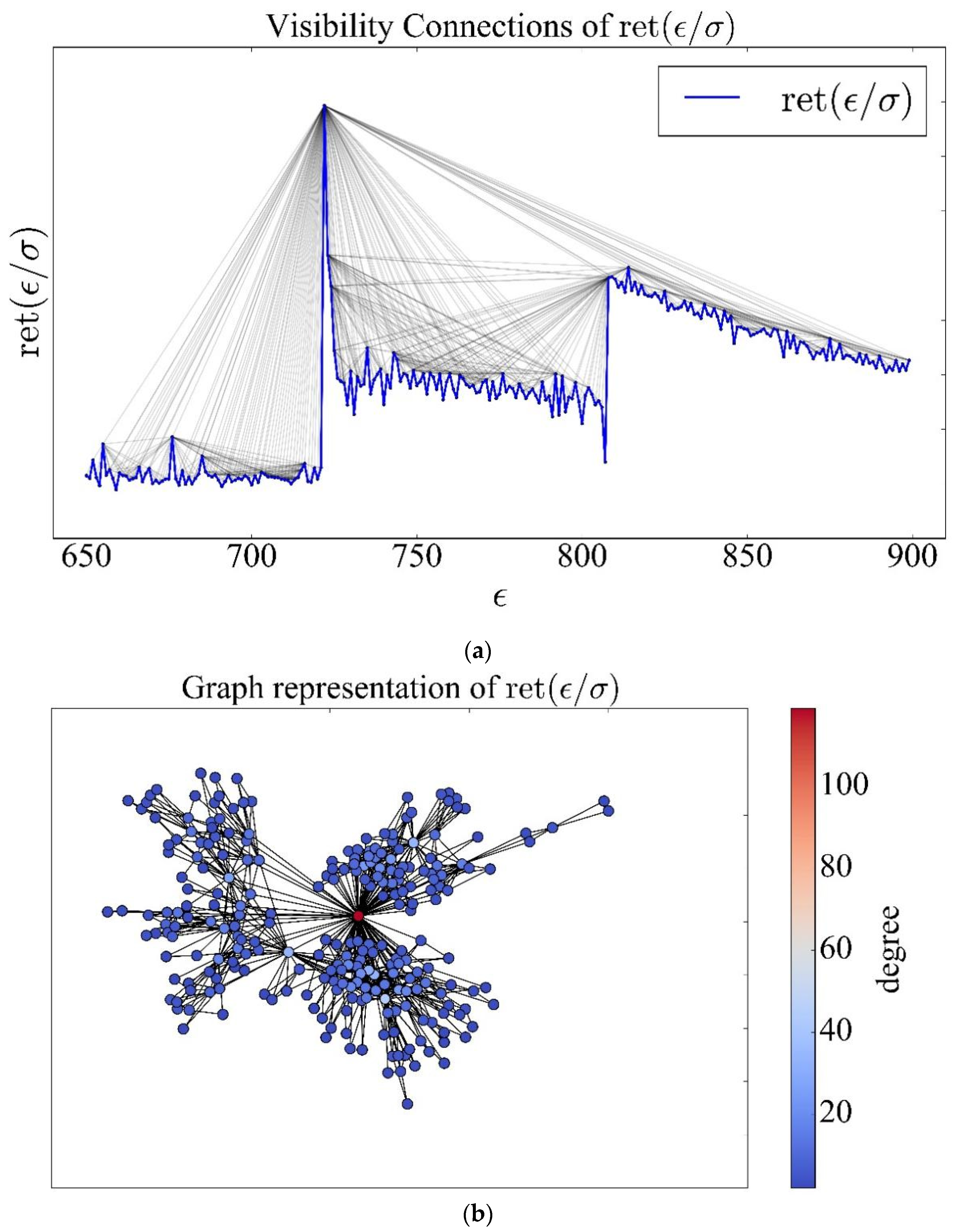
Further, we would like to present the results of the computations according to the described methodology and graph-based measures. First, we would like to present the visibility relationships between the values of the stress–strain curve based on the approaches of the VG. Moreover, we have to see the graph-like topology of the most important self-organization processes during the stretching of the material: transition from elastic to plastic regime and the stage of fracture.
Figure 2 presents the visibility connections based on the VG approach during the stage of the transition from elastic to plastic regime and the graph representation of the studied fragment with the emphasized degree connection for each element of the series.
In Figure 2, we see that the studied transition has a high degree of visibility. The degree of connectivity between each element is presented to be ununiform. According to Figure 2a, only one of the highest elements has the highest degree of visibility (connectivity) among other units. We can conclude that this point “sees” all other elements in a predefined range (window). The graph representation presented in Figure 2b gives the same conclusion about the studied transition. The color bar of Figure 2b gives us the notion that one element among others has the degree of connection that exceeds more than a hundred different elements. Based on this, we can understand that during the transition to plastic deformation, certain kinds of effects appear that form a complex, self-organizing dynamics on all metal surfaces. This leads to further irreversible processes of deformation of the material.
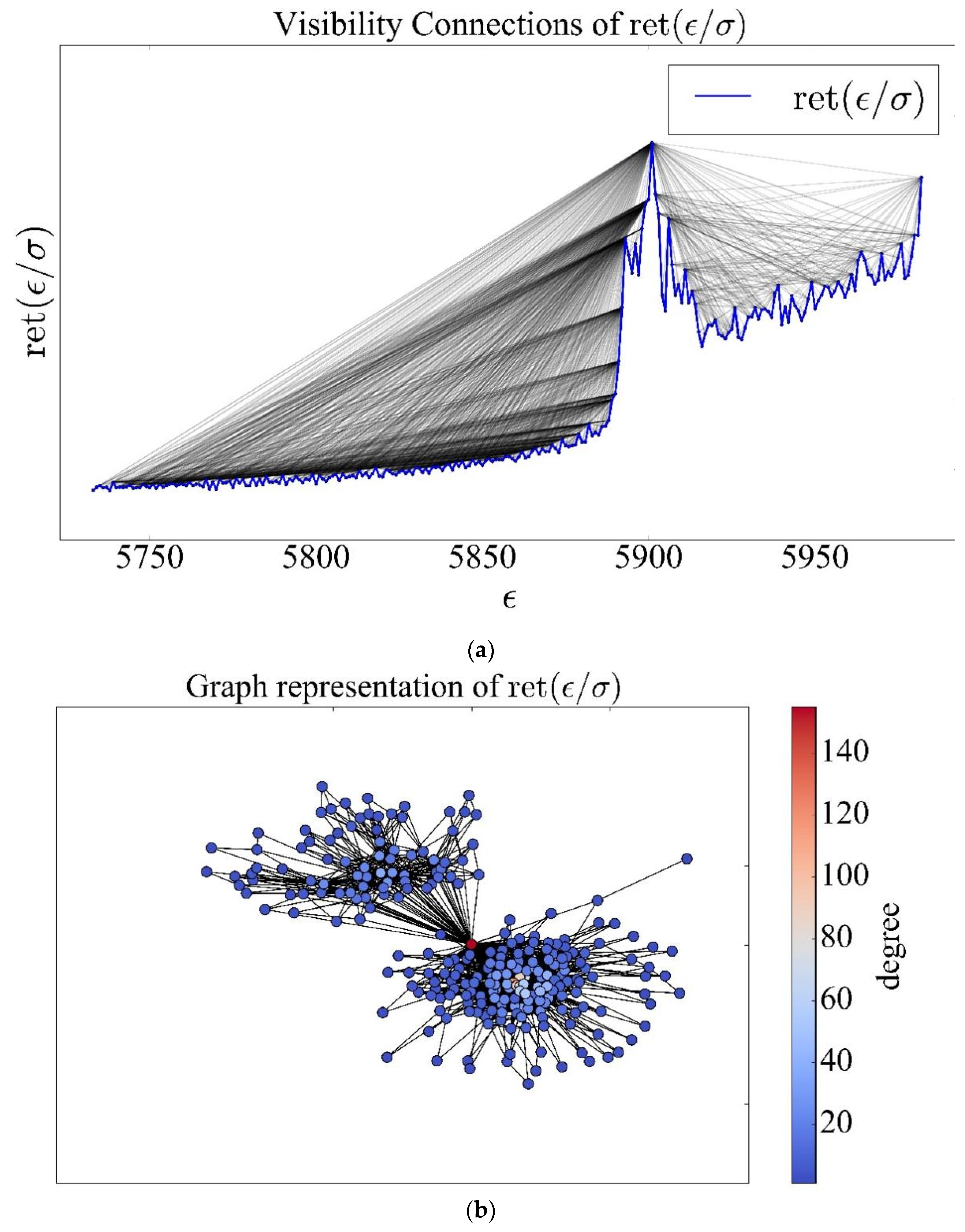
In Figure 3 are presented the visibility connections and the graph representation based on the VG approach for the last stage of interest—the stage of fracture.
In Figure 3a, we see that the dislocations that accumulate and lead to the fracture point are characterized by high visibility relation concentrated in several points before the total destruction of the material. In Figure 3b, we may see that one point is connecting two hubs (clusters) with a low degree of concentration. These clusters characterize periods before and after the highest point in the time series of the curve. The highest node is the linking point between these two clusters, which can serve as an indicator of highly self-organized dynamics before the crash. This is very similar to the first stage of interest.
The first and last stages of the system’s destruction remind us of the network model proposed by Barabási and Albert [89], for which the degree distribution P d is characterized by a heavy-tailed distribution—i.e., some vertices are highly connected while others have few connections—with the absence of a characteristic degree. The networks of such systems have been called scale-free. The degree distribution for such systems follows a power law distribution:
P d = d γ .
Further, we will see, except for a high degree of particular nodes, that these stages can be characterized by both a high-clustering coefficient and small average path length, compared to random graphs. The visibility connections and graph-based representation regarding the RP approach give a representation similar to the classical VG.
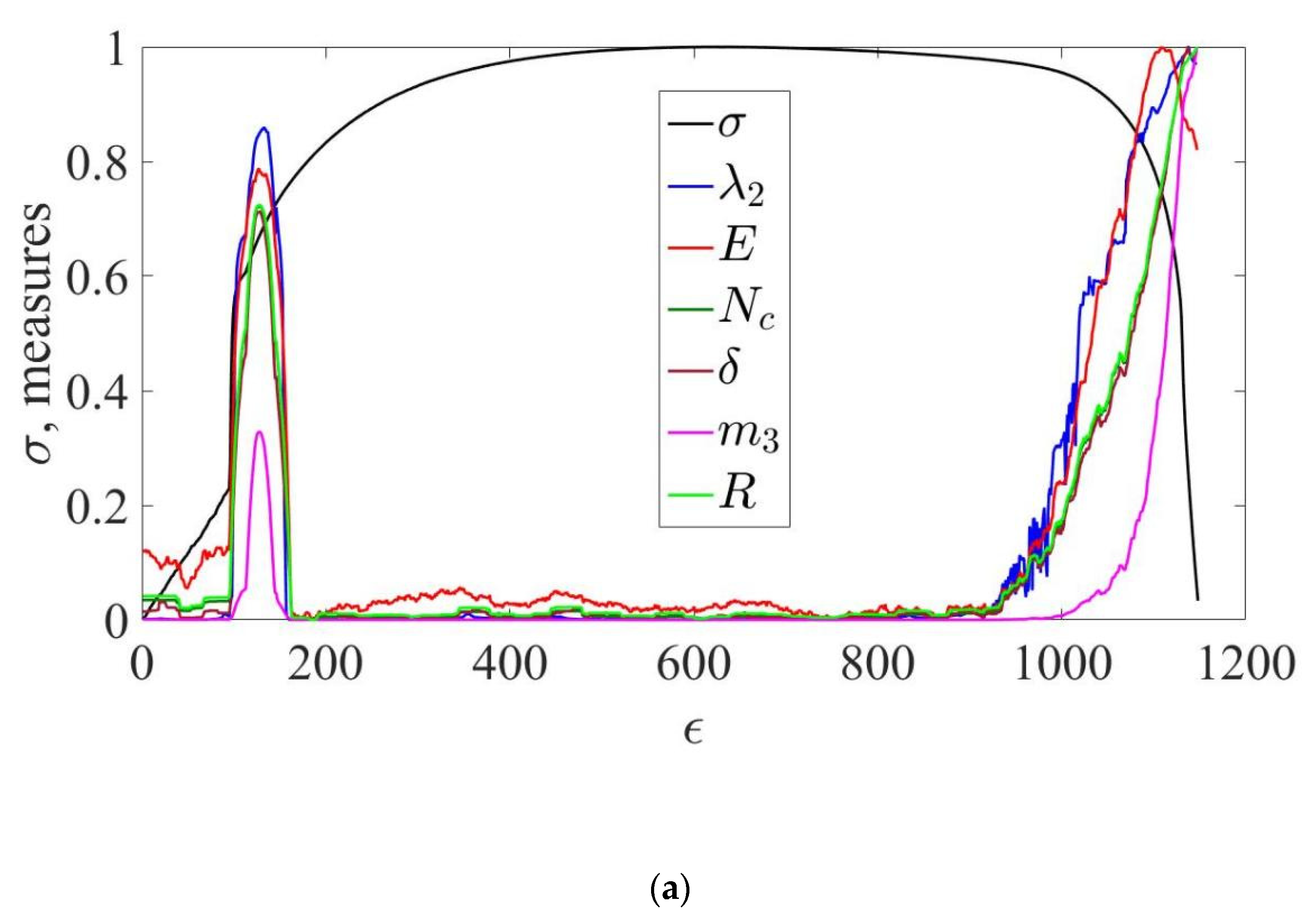
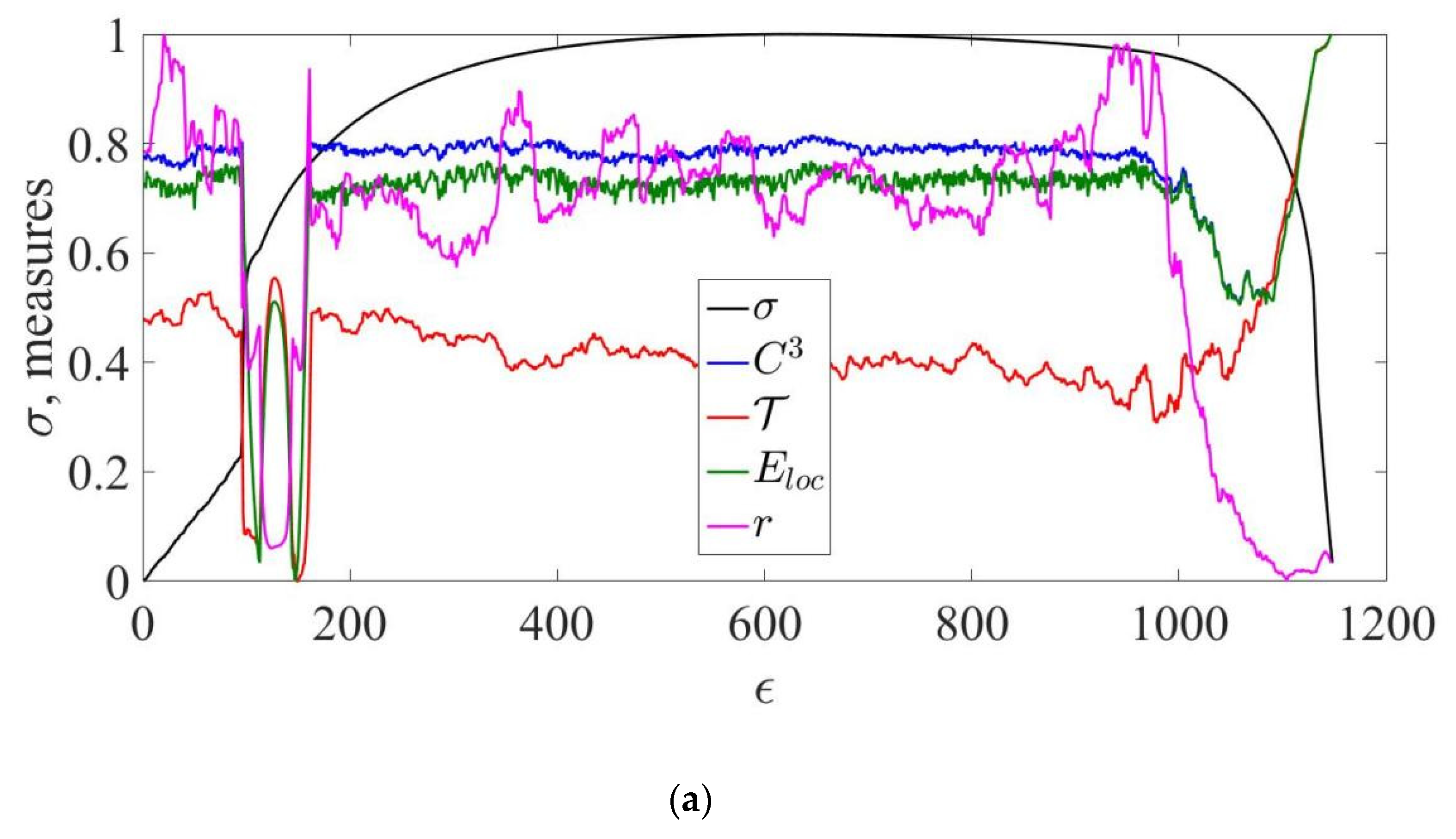
Next, we would like to present the comparative dynamics of the indicators (indicators-precursors) of the graph-based approaches described above along with the stress–strain curve. The presented indicators, as has already been described in Section 3, are calculated in accordance with the sliding window procedure in order to be able to track the change in the complexity of the system during the destruction of the metal. In Figure 4 are presented the spectral measures of complexity (in accordance with Section 4.3) based on the VG approach.
Figure 4 presents that the spectral indicators of complexity start to increase during the stages of interest—the transition from elastic to plastic deformation and the stage of fracture. Since all of them are based on the eigenvalues of the Laplacian matrix and the adjacency matrix, they behave synchronically during the studied series. We see that, as an example, λ 2 indicates the higher synchronizability and connectedness of the networks of those self-organized phenomena. The natural connectivity N c (see Equation (13)) demonstrates that the rate of developing of the self-organized dynamics far from equilibrium state is increasing. The energy of a graph E (see Equation (10)) shows that the overall amount of non-zero eigenvalues is increasing, which is an indication of growing complexity. The third spectral moment and other indicators indicate the development of an increase in the variability of alternative shortest paths, which is an indicator of the inhomogeneous effects’ development in the stages of interest. Before the point of fracture, nearly all measures rise before the exact breaking point. Having more data than the stress–strain curve, spectral measures can serve not just as indicators, but also as precursors of catastrophic phenomena.
Further, we would like to present topological measures of complexity based on the VG approach. Figure 5 shows the dynamics of maximum node degree ( D m a x ), global closeness centrality ( C ), global harmonic centrality ( G H c ), overall network information centrality ( I ), global efficiency ( E g l o b ), density ( ρ ), average degree connectivity ( d ¯ w ), and squares clustering coefficient ( C 4 ), along with the stress–strain curve.
In Figure 5, we may see that nearly all centrality measures increase during the stages of transition and fracture.
The maximum degree D m a x (see Equation (16)) behaves consistently with the graph representation of all stages: during the first and last stages, few extremely concentrated points appear, which may correspond to several defects that lead the entire dynamics of the system to a state far from equilibrium. The stages of strain hardening and necking appear to be the most inefficient in terms of networks. The graph representation of the stage of strain hardening demonstrated that the visibility connections among each vertex of the network are distributed uniformly. In accordance with our results, the defects on the surface of the material have to be distributed homogeneously during this stage. The last stage is compatible with the first one: wide-ranging self-organization of defects before the fracture of the metal is reflected in the increase of concentration for a particular node.
The high global closeness centrality of the network C (see Equation (18)) indicates that the defects during the stages of interest become more interconnected. One of the main cracks is the catalyst for all other events in the dynamics of metal destruction. If the closeness is small, then the farness of nodes is large and, perhaps, units of the studied system are independent of each other. Global harmonic centrality G H c based on standard harmonic centrality (see Equation (19)) is nearby to global closeness centrality in this sense.
The global information centrality I (see Equation (26)) is an indicator of the information flow in the network. The higher it is, the more efficient the transfer of information among different units of the network. We see that during the stages of transfer and before the fracture point, it grows, indicating the path length of the network to be shorter and some of the vertices to be frequently reachable. The idea of this indicator is the same as for previous ones. It’s especially similar to the closeness centrality [90,91].
Figure 5 presents to us that globally the stage of the transition and the stage of fracture appear to be efficient. Since global efficiency E g l o b (see Equation (33)) is the average of the characteristic path length among all nodes, and the average path length declines during corresponding periods, global interconnections (path) between the central node and other components are presented to be short and abundant. As already mentioned, during these stages, a leading dislocation appears, which is a reference point for the appearance of all subsequent ones.
Both the transition from elastic to plastic region and the stage of fracture are presented to be highly dense, according to ρ (see Equation (35)). We could see from previous results that these stages represent several highly interconnected nodes with a large degree of connectedness, clustering coefficient, low average path length, high global efficiency, etc. This measure only confirms our observations. It can be seen that the presented measure is almost close to one. This suggests that almost every dislocation (node in the graph) interacts with the rest of the nodes. This indicates a high degree of long-term memory during the processes of destruction in metals.
The average degree connectivity d ¯ w (see Equation (36)) shows that during the stage of transition of the stage of fracture, the connectedness between neighbors of a particular node i starts to increase, indicating the rise of complexity in given periods of deformation.
We see that the global clustering coefficient of squared clusters C 4 (see Equation (31)) rises during the stages of interest, showing us that their network representations follow a scale-free model, but the interconnections between nodes of their network form a much more complex structure. The topology of our network can follow a monopartite structure. As an example, as we can see from Figure 4b, there are approximately two hubs in our network that are connected by particularly extremely connected nodes that see all other nodes. These two hubs can correspond to the periods before the last most serious crack and those defects that are consequences of this cracking. All of them are presented to be interconnected through the final crack which has led to the point of fracture. Thus, we should consider these measures simultaneously as the complexity of any studied process can be variative, and different phenomena can result in a variative topology of the network, which reflects the studied process.
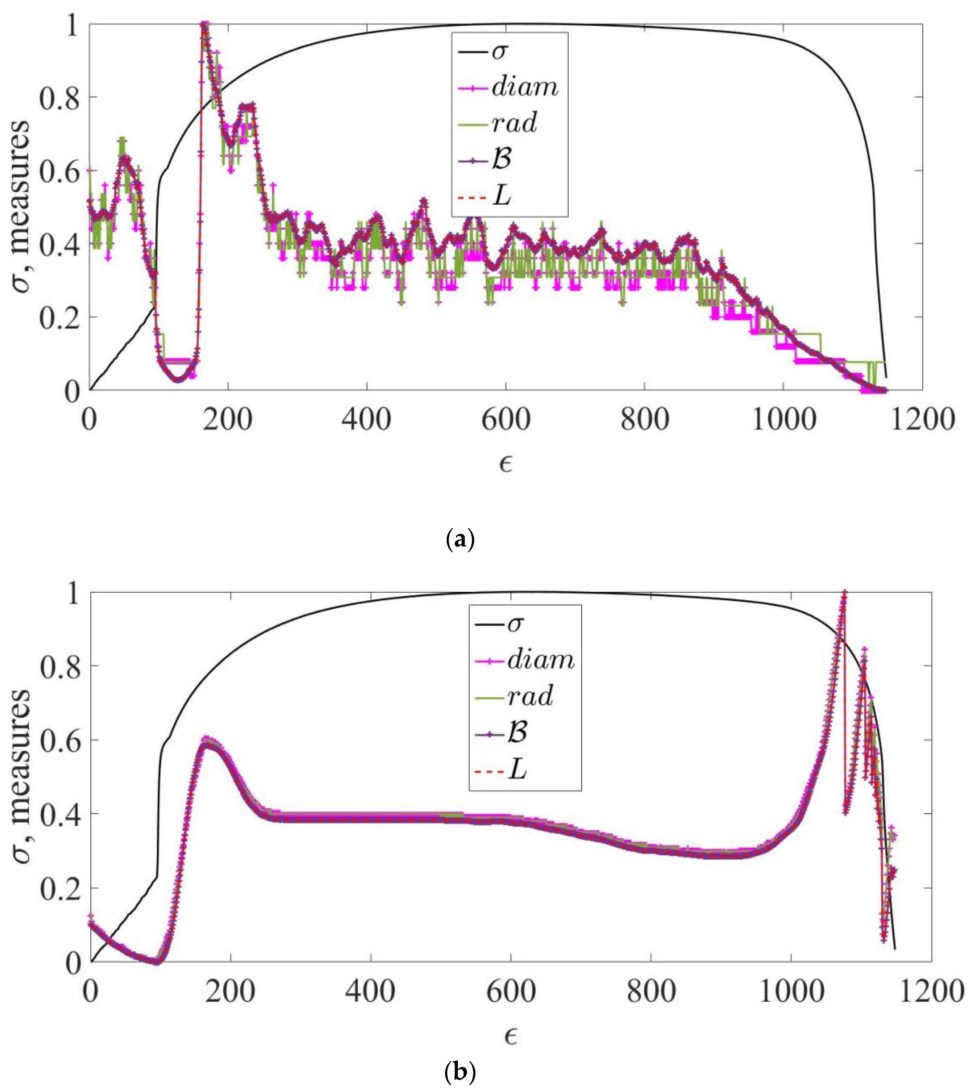
In Figure 6 is presented the dynamics of diameter ( d i a m ), radius ( r a d ), global betweenness centrality ( B ), and average shortest path length ( L ), along with the stress–strain curve.
From Figure 6a we can see that the average path length L (see Equation (27)) between each vertex of the network decreases during the transition from the elastic to plastic deformation and before the fracture point. As was mentioned previously, according to this measure, the network in general becomes more efficient during these stages. The rate of information flow between each defect appears to be more abrupt, compared to other periods, where the visibility connections between nodes are distributed in a more uniform manner. This makes particular vertices very remotely connected to others.
Figure 6b presents that at the stage of transition, the average shortest path length for the RP approach is precisely the same as for the VG, whereas just before the rupture, it starts to increase. We can assume that in the recurrence graph, the nodes of the network are connected only to their two closest neighbors in front and behind. That is, there are practically no workarounds to the third vertex in this graph, which is why the average number of steps taken to move from one vertex to another increases.
We have already mentioned that the diameter ( d i a m ) of the network (see Equation (39)) is the longest path lengths among all other paths. The radius ( r a d ) (see Equation (40)) represents the minimal among the longest paths. Both measures are based on the eccentricity of the nodes, which in turn is based on the shortest path lengths of the network under study. Since the path length decreases during periods of self-organization of the system, which is also reflected in an increase in the density of nodes and their closeness, the measures presented should also decrease in the stages of interest to us, which we see in Figure 6a.
In accordance with the previous results for a recurrent network, considering such approaches as global efficiency, the average shortest path length, global clustering coefficient of squared clusters, etc., we see that d i a m and r a d behave in a similar way to the visibility graph during the transition from elastic to plastic deformation. The asymmetry in the dynamics of the two approaches is observed only before the breaking point.
In Figure 6a, the global betweenness centrality B (see Equation (21)) shows that, on average, the number of paths passing through a particular node is falling. This can be interpreted in such a way that one specific effect appears in the dynamics of metal destruction, which begins to be responsible for absolutely all processes taking place during stretching. According to our results, it forms a highly centered network topology, where almost all information passes through one node. At the same time, the other nodes (defects), observing the leader among all, behave consistently, but, as the graph shows, the number of paths for their cooperation should not be excessively large. It is enough for a couple of paths directed at each other and at the most informative among all defects. In Figure 6b, we can see precisely the same pattern. However, at the stage of fracture, it grows. Perhaps it indicates that in a non-linear topology of the network, some nodes in the area of the highest concentration get the largest flow of information (fraction of paths) through themselves from distant ones. At the exact point of fracture, B for the RP approach acts in the same way as for the VG.
In Figure 7 are presented clustering-based measures of complexity, such as C 3 and T with local efficiency E l o c and assortativity coefficient r , along with the stress–strain curve.
From Figure 7, we see that the global clustering coefficient of triangle cliques C 3 (see Equation (29)) decreases during the stages of self-organized transition from the elastic to the plastic region and before the point of fracture. As we have concluded, those periods are the representatives of scale-free networks. Our empirical results present that the degree distribution of those stages follows a power law (see Equation (41)), and the average shortest path length (see Figure 6) declines, indicating that the rate of information flow increases during them, which results in highly complex, self-organized phenomena. In this case, we would expect our defects to form clusters for which C 3 increased. Nevertheless, the topology of our network that reflects the studied stages is presented to be much more complex. As was discussed in Section 4.4.3, the triangle clusters may be abundant in a monopartite network, while they may be absent in bipartite networks [82,83].
Relying on the results presented in Figure 5b and Figure 7b, we see that at the stage of the transition, the network demonstrates bivariate clustering—both triangle and square clustering. On the threshold of the fracture itself, it is clear that the number of clusters of both types decline, and only at the point of the fracture itself, the concentration of clusters increases again. Based on the topology of a recurrence network, it can be assumed that its nonlinearly shaped form, which is reduced to a small, highly concentrated cluster of points, cannot have a sufficient number of clusters in this form. In such a graph, everyone can be connected to everyone only through one specific direct path and there are no bypass shortest paths.
Since the transitivity T (see Equation (30)) is the modification of C 3 , it demonstrates related to the standard clustering coefficient dynamics.
Locally, according to E l o c (see Equation (34)), our stages seem to be inefficient. Local efficiency is the average efficiency of information transfer within local subgraphs G i . Low local efficiency for the periods of interest to us may indicate that although globally different nodes of the network are well interconnected with a certain central one, in local subgraphs of the network many nodes do not interact with each other sufficiently. The reference point of their chaotic, self-organized behavior is the global dislocation, on the basis of which most communication clusters are built. It is worth mentioning that the stage of the transition for RP seems to be efficient enough according to both E g l o b and E l o c . Observing the clustering coefficients, we can say that according to the recurrence approach, each of the nodes is interconnected. The recurrent map may reflect the fact that each of the dislocations interacts with the others in full during the processes of self-organization when moving from elastic to plastic deformation, while for the stage of fracture only few nodes matter in this process.
Figure 7a demonstrates that the assortativity coefficient r (see Equation (37)) decreases during stages of interest. It implies that most low-connected nodes (dislocations) have the tendency to follow dislocation with the highest influence. The opposite condition is also true. As an example, after the transition from the elastic to the plastic deformation, we would expect strain hardening for which visibility connections would lead from the highest node to the smallest ones (with low degree). During this process, the movement of small dislocations would matter. The dynamics of d ¯ w (see Figure 5) is inconsistent with our observation and assumptions and would require additional research in the future. Nevertheless, as an indicator (indicator-precursor), it has declines and increases in those stages that we are trying to identify and classify.
The result of the dynamics of the assortativity coefficient for the recurrence approach (see Figure 7b) is also slightly inconsistent with the dynamics of the visibility graph. Based on this, it becomes extremely urgent to include additional approaches to converting a time series into a graph.

6. Conclusions

In this study, we have presented the measures of a quantitative assessment of chaotic, irreversible, and self-organized deformation processes in metals using complex network methods. Here, we have studied the possibility of using two types of complex network indicators—spectral and topological. To the group of spectral measures, we have included the following: algebraic connectivity, energy of the graph, spectral gap, spectral radius, natural connectivity, and k -th spectral moment. The group of topological measures included maximum degree centrality, global closeness centrality, global harmonic centrality, global betweenness centrality, global network information centrality, average shortest path length, global clustering coefficient of triangle clusters, transitivity, global clustering coefficient of squared clusters, global and local efficiencies, density, average degree connectivity, assortativity coefficient, diameter, and radius. The presented measures of complexity were found to be especially informative. They can be used not only for monitoring and classifying the stages of deformation, but also their applicability extends to the terms of a precursor of the deformation stages during plastic deformation in the metal. These indicators-precursors can be used in the development of technical devices for early diagnosis of catastrophic processes of material destruction. We have tested the possibility to detect periods of high concentration of defects and their self-organization with the presented measures on the example of the stress–strain curve time series σ ϵ for DC04 steel. Our results have shown that the regimes of the transition from the elastic to the plastic region and the fracture area are presented to be highly clustered, efficient, concentrated, dense, and self-organized, whereas all other regimes seem to be globally random.
We could see that the emergence and development of defect structures that appear during the deformation of metals form complex, nonlinear, heterogenous, i.e., self-organized, dynamics, which is far from thermodynamic equilibrium. The identified regimes of self-organization (instability) are characterized by the asymmetry in their dynamics and low entropy production in the development of metal, and are supported by a high auto-correlation (long-term memory) effect.
Further, it would be interesting to study inhomogeneous defect structure formation with the usage of multifractal theory [40,43,92,93,94,95,96,97], information theory [40,44,45,46,48,49], additional approaches in complex network theory [41,42,44], chaos theory [47], theory of irreversibility [42], and machine (deep) learning [98,99,100].

Author Contributions

Conceptualization, A.K., V.S. and A.B. (Andrii Bielinskyi); methodology, V.S. and A.B. (Andrii Bielinskyi); software, A.B. (Andrii Bielinskyi); validation, A.K., A.B. (Arkady Bryukhanov), V.S., A.B. (Andrii Bielinskyi), T.K., D.D., I.D. and V.L.; formal analysis, A.K., A.B. (Arkady Bryukhanov), V.S., A.B. (Andrii Bielinskyi), T.K., D.D., I.D. and V.L.; investigation, A.K., A.B. (Arkady Bryukhanov), V.S., A.B. (Andrii Bielinskyi), T.K., D.D., I.D. and V.L.; resources, V.S. and A.B. (Andrii Bielinskyi); data curation, V.S. and A.B. (Andrii Bielinskyi); writing—original draft preparation, V.S. and A.B. (Andrii Bielinskyi); writing—review and editing, A.K., A.B. (Arkady Bryukhanov), V.S., A.B. (Andrii Bielinskyi), T.K., D.D., I.D. and V.L.; visualization, A.B. (Andrii Bielinskyi); supervision, A.K. and V.S.; project administration, A.K. and V.S.; funding acquisition, V.S. All authors have read and agreed to the published version of the manuscript.

Funding

This work was supported in part by the Ministry of Education and Science of Ukraine (projects No. 0121U109543, 0122U000850, and 0122U000874) and National Research Foundation of Ukraine (project No. 2020.02/0100). T.K. also acknowledges the SAIA (Slovak Academic Information Agency) for scholarship in the Institute of Physics of Slovak Academy of Sciences in the framework of the National Scholarship Programme of the Slovak Republic.

Data Availability Statement

The data used in this study can be found at the corresponding link: https://github.com/Butman2099/Complex-systems-measures/tree/main/Data%20Dynamics%20MDPI%202022 (accessed on 27 January 2023).

Conflicts of Interest

The authors declare no conflict of interest. The funders had no role in the design of the study; in the collection, analyses, or interpretation of data; in the writing of the manuscript; or in the decision to publish the results.

References

  1. Hawking, S. I Think the Next Century Will Be the Century of Complexity. What Is Complexity? San José Mercury News, 23 January 2000. [Google Scholar]
  2. Holovatch, Y.; Kenna, R.; Thurner, S. Complex Systems: Physics beyond Physics. Eur. J. Phys. 2017, 38, 023002. [Google Scholar] [CrossRef]
  3. Kwapień, J.; Drożdż, S. Physical Approach to Complex Systems. Phys. Rep. 2012, 515, 115–226. [Google Scholar] [CrossRef]
  4. Sinatra, R.; Deville, P.; Szell, M.; Wang, D.; Barabási, A.-L. A Century of Physics. Nat. Phys. 2015, 11, 791–796. [Google Scholar] [CrossRef]
  5. Kolmogorov, A.N. Three Approaches to the Quantitative Definition of Information. Int. J. Comput. Math. 1968, 2, 157–168. [Google Scholar] [CrossRef]
  6. Anderson, P.W. More Is Different. Science 1972, 177, 393–396. [Google Scholar] [CrossRef] [PubMed] [Green Version]
  7. Prigogine, I. Exploring Complexity. Eur. J. Oper. Res. 1987, 30, 97–103. [Google Scholar] [CrossRef]
  8. Gell-Mann, M. What Is Complexity? Remarks on Simplicity and Complexity by the Nobel Prize-Winning Author of The Quark and the Jaguar. Complexity 1995, 1, 16–19. [Google Scholar] [CrossRef]
  9. Parisi, G. Complex Systems: A Physicist’s Viewpoint. Phys. A 1999, 263, 557–564. [Google Scholar] [CrossRef] [Green Version]
  10. Zeng, A.; Shen, Z.; Zhou, J.; Wu, J.; Fan, Y.; Wang, Y.; Stanley, H.E. The Science of Science: From the Perspective of Complex Systems. Phys. Rep. 2017, 714–715, 1–73. [Google Scholar] [CrossRef]
  11. Sayama, H. Introduction to the Modeling and Analysis of Complex Systems; Open Suny Textbooks, Milne Library, State University Of New York: Geneseo, NY, USA, 2015. [Google Scholar]
  12. Estrada, E. Graph and Network Theory in Physics. Available online: https://arxiv.org/abs/1302.4378 (accessed on 18 June 2013).
  13. Boccara, N. Modelling Complex Systems; Springer: New York, NY, USA, 2010. [Google Scholar]
  14. Latora, V.; Nicosia, V.; Russo, G. Complex Networks: Principles, Methods and Applications; Cambridge University Press: Cambridge, UK, 2017. [Google Scholar]
  15. Donner, R.V.; Small, M.; Donges, J.F.; Marwan, N.; Zou, Y.; Xiang, R.; Kurths, J. Recurrence-Based Time Series Aanalysis by Means of Complex Network Methods. Int. J. Bifurcat. Chaos 2011, 21, 1019–1046. [Google Scholar] [CrossRef]
  16. Lacasa, L.; Nuñez, A.; Roldán, É.; Parrondo, J.M.R.; Luque, B. Time Series Irreversibility: A Visibility Graph Approach. Eur. Phys. J. B 2012, 85, 217. [Google Scholar] [CrossRef] [Green Version]
  17. Varley, T.F.; Sporns, O. Network Analysis of Time Series: Novel Approaches to Network Neuroscience. Front. Neurosci. 2022, 15, 787068. [Google Scholar] [CrossRef] [PubMed]
  18. Zou, Y.; Donner, R.V.; Marwan, N.; Donges, J.F.; Kurths, J. Complex Network Approaches to Nonlinear Time Series Analysis. Phys. Rep. 2019, 787, 1–97. [Google Scholar] [CrossRef]
  19. Li, M.; Liu, R.-R.; Lü, L.; Hu, M.-B.; Xu, S.; Zhang, Y.-C. Percolation on Complex Networks: Theory and Application. Phys. Rep. 2021, 907, 1–68. [Google Scholar] [CrossRef]
  20. Wang, W.; Liu, Q.-H.; Liang, J.; Hu, Y.; Zhou, T. Coevolution Spreading in Complex Networks. Phys. Rep. 2019, 820, 1–51. [Google Scholar] [CrossRef]
  21. Battiston, F.; Amico, E.; Barrat, A.; Bianconi, G.; Ferraz de Arruda, G.; Franceschiello, B.; Iacopini, I.; Kéfi, S.; Latora, V.; Moreno, Y.; et al. The Physics of Higher-Order Interactions in Complex Systems. Nat. Phys. 2021, 17, 1093–1098. [Google Scholar] [CrossRef]
  22. Battiston, F.; Petri, G. Higher-Order System (Understanding Complex Systems), 1st ed.; Springer: Cham, Switzerland, 2022. [Google Scholar]
  23. Vinogradov, A.; Yasnikov, I.S.; Estrin, Y. Stochastic Dislocation Kinetics and Fractal Structures in Deforming Metals Probed by Acoustic Emission and Surface Topography Measurements. J. Appl. Phys. 2014, 115, 233506. [Google Scholar] [CrossRef]
  24. Papadopoulos, L.; Porter, M.A.; Daniels, K.E.; Bassett, D.S. Network Analysis of Particles and Grains. J. Complex Netw. 2018, 6, 485–565. [Google Scholar] [CrossRef] [Green Version]
  25. Papadopoulos, L.; Puckett, J.G.; Daniels, K.E.; Bassett, D.S. Evolution of Network Architecture in a Granular Material under Compression. Phys. Rev. E 2016, 94, 032908. [Google Scholar] [CrossRef] [Green Version]
  26. Giusti, C.; Papadopoulos, L.; Owens, E.T.; Daniels, K.E.; Bassett, D.S. Topological and Geometric Measurements of Force-Chain Structure. Phys. Rev. E 2016, 94, 032909. [Google Scholar] [CrossRef]
  27. Walker, D.M.; Tordesillas, A.; Small, M.; Behringer, R.P.; Tse, C.K. A Complex Systems Analysis of Stick-Slip Dynamics of a Laboratory Fault. Chaos Int. J. Nonlin. Sci. 2014, 24, 013132. [Google Scholar] [CrossRef] [PubMed] [Green Version]
  28. Kryven, I.; Duivenvoorden, J.; Hermans, J.; Iedema, P.D. Random Graph Approach to Multifunctional Molecular Networks. Macromol. Theory Simul. 2016, 25, 449–465. [Google Scholar] [CrossRef]
  29. Tordesillas, A.; Walker, D.M.; Andò, E.; Viggiani, G. Revisiting Localized Deformation in Sand with Complex Systems. Proc. R. Soc. A Math. Phys. Eng. Sci. 2013, 469, 20120606. [Google Scholar] [CrossRef]
  30. Karapiperis, K.; Andrade, J.E. Nonlocality in Granular Complex Networks: Linking Topology, Kinematics and Forces. Extreme Mech. Lett. 2021, 42, 101041. [Google Scholar] [CrossRef]
  31. Zhang, Z.; Qin, Y.; Jia, L.; Chen, X. Visibility Graph Feature Model of Vibration Signals: A Novel Bearing Fault Diagnosis Approach. Materials 2018, 11, 2262. [Google Scholar] [CrossRef] [Green Version]
  32. Mohebian, P.; Aval, S.B.B.; Noori, M.; Lu, N.; Altabey, W.A. Visible Particle Series Search Algorithm and Its Application in Structural Damage Identification. Sensors 2022, 22, 1275. [Google Scholar] [CrossRef]
  33. Walker, D.M.; Tordesillas, A.; Pucilowski, S.; Lin, Q.; Rechenmacher, A.L.; Abedi, S. Analysis of Grain-Scale Measurements of Sand Using Kinematical Complex Networks. Int. J. Bifurcat. Chaos 2012, 22, 1230042. [Google Scholar] [CrossRef]
  34. Meng, F.; Terentjev, E. Transient Network at Large Deformations: Elastic–Plastic Transition and Necking Instability. Polymers 2016, 8, 108. [Google Scholar] [CrossRef] [Green Version]
  35. Ghaffari, H.O.; Young, R.P. Acoustic-Friction Networks and the Evolution of Precursor Rupture Fronts in Laboratory Earthquakes. Sci. Rep. 2013, 3, 1799. [Google Scholar] [CrossRef] [Green Version]
  36. Zuev, L.B.; Barannikova, S.A. Autowave Physics of Material Plasticity. Crystals 2019, 9, 458. [Google Scholar] [CrossRef]
  37. Sendrowicz, A.; Myhre, A.O.; Wierdak, S.W.; Vinogradov, A. Challenges and Accomplishments in Mechanical Testing Instrumented by In Situ Techniques: Infrared Thermography, Digital Image Correlation, and Acoustic Emission. Appl. Sci. 2021, 11, 6718. [Google Scholar] [CrossRef]
  38. Olemskoi, A.I.; Sklyar, I.A. Evolution of the defect structure of a solid during plastic deformation. Sov. Phys. Usp. 1992, 35, 455–480. [Google Scholar] [CrossRef]
  39. Kocańda, A.; Jasiński, C. Extended Evaluation of Erichsen Cupping Test Results by Means of Laser Speckle. Arch. Civ. Mech. Eng. 2016, 16, 211–216. [Google Scholar] [CrossRef]
  40. Bielinskyi, A.; Semerikov, S.; Serdyuk, O.; Solovieva, V.; Soloviev, V.; Pichl, L. Econophysics of sustainability indices. CEUR Workshop Proc. 2020, 2713, 372–392. [Google Scholar]
  41. Bielinskyi, A.; Soloviev, V. Complex network precursors of crashes and critical events in the cryptocurrency market. CEUR Workshop Proc. 2018, 2292, 37–45. [Google Scholar]
  42. Bielinskyi, A.O.; Hushko, S.V.; Matviychuk, A.V.; Serdyuk, O.A.; Semerikov, S.O.; Soloviev, V.N. Irreversibility of financial time series: A case of crisis. CEUR Workshop Proc. 2021, 3048, 134–150. [Google Scholar]
  43. Bielinskyi, A.O.; Serdyuk, O.A.; Semerikov, S.O.; Soloviev, V.N. Econophysics of cryptocurrency crashes: A systematic review. CEUR Workshop Proc. 2021, 3048, 31–133. [Google Scholar]
  44. Soloviev, V.N.; Belinskiy, A. Complex Systems Theory and Crashes of Cryptocurrency Market. In Information and Communication Technologies in Education, Research, and Industrial Applications; Springer: Cham, Switzerland, 2019; pp. 276–297. [Google Scholar] [CrossRef]
  45. Soloviev, V.; Belinskij, A. Methods of nonlinear dynamics and the construction of cryptocurrency crisis phenomena precursors. CEUR Workshop Proc. 2018, 2104, 116–127. [Google Scholar]
  46. Soloviev, V.; Bielinskyi, A.; Kharadzjan, N. Coverage of the coronavirus pandemic through entropy measures. CEUR Workshop Proc. 2020, 2832, 24–42. [Google Scholar]
  47. Soloviev, V.; Bielinskyi, A.; Serdyuk, O.; Solovieva, V.; Semerikov, S. Lyapunov exponents as indicators of the stock market crashes. CEUR Workshop Proc. 2020, 2732, 455–470. [Google Scholar]
  48. Soloviev, V.; Bielinskyi, A.; Solovieva, V. Entropy analysis of crisis phenomena for DJIA index. CEUR Workshop Proc. 2019, 2393, 434–449. [Google Scholar]
  49. Soloviev, V.; Serdiuk, O.; Semerikov, S.; Kohut-Ferens, O. Recurrence entropy and financial crashes. Adv. Econ. Bus. Manag. Res. 2019, 99, 385–388. [Google Scholar] [CrossRef] [Green Version]
  50. Kennel, M.B.; Brown, R.; Abarbanel, H.D.I. Determining Embedding Dimension for Phase-Space Reconstruction Using a Geometrical Construction. Phys. Rev. A 1992, 45, 3403–3411. [Google Scholar] [CrossRef] [Green Version]
  51. Fraser, A.M.; Swinney, H.L. Independent Coordinates for Strange Attractors from Mutual Information. Phys. Rev. A 1986, 33, 1134–1140. [Google Scholar] [CrossRef] [PubMed]
  52. Donges, J.F.; Heitzig, J.; Donner, R.V.; Kurths, J. Analytical Framework for Recurrence Network Analysis of Time Series. Phys. Rev. E 2012, 85, 046105. [Google Scholar] [CrossRef] [PubMed] [Green Version]
  53. Donner, R.V.; Zou, Y.; Donges, J.F.; Marwan, N.; Kurths, J. Ambiguities in Recurrence-Based Complex Network Representations of Time Series. Phys. Rev. E 2010, 81, 015101. [Google Scholar] [CrossRef] [Green Version]
  54. Jacob, R.; Harikrishnan, K.P.; Misra, R.; Ambika, G. Cross over of Recurrence Networks to Random Graphs and Random Geometric Graphs. Pramana 2017, 88, 37. [Google Scholar] [CrossRef]
  55. Marwan, N.; Carmenromano, M.; Thiel, M.; Kurths, J. Recurrence Plots for the Analysis of Complex Systems. Phys. Rep. 2007, 438, 237–329. [Google Scholar] [CrossRef]
  56. Schinkel, S.; Dimigen, O.; Marwan, N. Selection of Recurrence Threshold for Signal Detection. Eur. Phys. J. Spec. Top. 2008, 164, 45–53. [Google Scholar] [CrossRef]
  57. Eroglu, D.; Marwan, N.; Prasad, S.; Kurths, J. Finding Recurrence Networks’ Threshold Adaptively for a Specific Time Series. Nonlinear Process. Geophys. 2014, 21, 1085–1092. [Google Scholar] [CrossRef] [Green Version]
  58. Jacob, R.; Harikrishnan, K.P.; Misra, R.; Ambika, G. Characterization of Chaotic Attractors under Noise: A Recurrence Network Perspective. Commun. Nonlinear Sci. Numer. Simul. 2016, 41, 32–47. [Google Scholar] [CrossRef]
  59. Jacob, R.; Harikrishnan, K.P.; Misra, R.; Ambika, G. Uniform Framework for the Recurrence-Network Analysis of Chaotic Time Series. Phys. Rev. E 2016, 93, 012202. [Google Scholar] [CrossRef] [PubMed] [Green Version]
  60. Lin, M.; Fan, X.X.; Wang, G.; Zhao, G. Network Structure Entropy and Its Dynamical Evolution for Recurrence Networks from Earthquake Magnitude Time Series. Eur. Phys. J. B 2016, 89, 131. [Google Scholar] [CrossRef]
  61. Da Costa, L.F.; Rodrigues, F.A.; Travieso, G.; Villas Boas, P.R. Characterization of Complex Networks: A Survey of Measurements. Adv. Phys. 2007, 56, 167–242. [Google Scholar] [CrossRef] [Green Version]
  62. Lacasa, L.; Luque, B.; Ballesteros, F.; Luque, J.; Nuño, J.C. From Time Series to Complex Networks: The Visibility Graph. Proc. Natl. Acad. Sci. USA 2008, 105, 4972–4975. [Google Scholar] [CrossRef] [Green Version]
  63. Lacasa, L.; Toral, R. Description of Stochastic and Chaotic Series Using Visibility Graphs. Phys. Rev. E 2010, 82, 036120. [Google Scholar] [CrossRef] [PubMed] [Green Version]
  64. Luque, B.; Lacasa, L.; Ballesteros, F.; Luque, J. Horizontal Visibility Graphs: Exact Results for Random Time Series. Phys. Rev. E 2009, 80, 046103. [Google Scholar] [CrossRef]
  65. Ott, E. Chaos in Dynamical Systems; Cambridge University Press: Cambridge, UK, 2002. [Google Scholar]
  66. Poincaré, H. Sur le problème des trois corps et les équations de la dynamique. Acta Math. 1890, 13, A3–A270. [Google Scholar]
  67. Eckmann, J.-P.; Kamphorst, S.O.; Ruelle, D. Recurrence Plots of Dynamical Systems. Europhys. Lett. 1987, 4, 973–977. [Google Scholar] [CrossRef] [Green Version]
  68. Chung, F.R.K. Spectral Graph Theory; American Mathematical Society: Providence, RI, USA, 1997. [Google Scholar]
  69. Biggs, N. Spectral Graph Theory (CBMS Regional Conference Series in Mathematics 92). Bull. Lond. Math. Soc. 1998, 30, 197–199. [Google Scholar] [CrossRef]
  70. Butler, S. Interlacing for Weighted Graphs Using the Normalized Laplacian. Electron. J. Linear Algebra 2007, 16, 90–98. [Google Scholar] [CrossRef] [Green Version]
  71. Bounova, G.; de Weck, O. Overview of Metrics and Their Correlation Patterns for Multiple-Metric Topology Analysis on Heterogeneous Graph Ensembles. Phys. Rev. E 2012, 85, 016117. [Google Scholar] [CrossRef] [PubMed]
  72. Gutman, I. The energy of a graph. Ber. Math. Statist. Sekt.-Ungszentram Graz. 1978, 103, 1–22. [Google Scholar]
  73. Jun, W.; Barahona, M.; Yue-Jin, T.; Hong-Zhong, D. Natural Connectivity of Complex Networks. Chin. Phys. Lett. 2010, 27, 078902. [Google Scholar] [CrossRef]
  74. Estrada, E. Spectral Scaling and Good Expansion Properties in Complex Networks. Europhys. Lett. 2006, 73, 649–655. [Google Scholar] [CrossRef] [Green Version]
  75. Wu, J.; Barahona, M.; Tan, Y.-J.; Deng, H.-Z. Spectral Measure of Structural Robustness in Complex Networks. IEEE Trans. Syst. Man Cybern. Part A Syst. Hum. 2011, 41, 1244–1252. [Google Scholar] [CrossRef]
  76. Cvetkovic, D.M.; Sachs, H.; Doob, M. Spectra of Graphs: Theory and Application; Academic Press Inc.: New York, NY, USA, 1979. [Google Scholar]
  77. Latora, V.; Marchiori, M. Efficient Behavior of Small-World Networks. Phys. Rev. Lett. 2001, 87, 198701. [Google Scholar] [CrossRef] [Green Version]
  78. Stephenson, K.; Zelen, M. Rethinking Centrality: Methods and Examples. Soc. Networks 1989, 11, 1–37. [Google Scholar] [CrossRef]
  79. Watts, D.J.; Strogatz, S.H. Collective dynamics of small-world networks. Nature 1998, 393, 440–442. [Google Scholar] [CrossRef]
  80. Barrat, A.; Weigt, M. On the properties of small-world network models. Eur. Phys. J. B 2000, 13, 547–560. [Google Scholar] [CrossRef] [Green Version]
  81. Boccaletti, S.; Latora, V.; Moreno, Y.; Chavez, M.; Hwang, D.-U. Complex networks: Structure and dynamics. Phys. Rep. 2006, 424, 175–308. [Google Scholar] [CrossRef]
  82. Holme, P.; Edling, C.R.; Liljeros, F. Structure and time evolution of an Internet dating community. Soc. Netw. 2004, 26, 155–174. [Google Scholar] [CrossRef] [Green Version]
  83. Holme, P.; Liljeros, F.; Edling, C.R.; Kim, B.J. Network bipartivity. Phys. Rev. E 2003, 68, 056107. [Google Scholar] [CrossRef] [PubMed] [Green Version]
  84. Lind, P.G.; González, M.C.; Herrmann, H.J. Cycles and clustering in bipartite networks. Phys. Rev. E 2005, 72, 056127. [Google Scholar] [CrossRef] [Green Version]
  85. Zhang, P.; Wang, J.; Li, X.; Li, M.; Di, Z.; Fan, Y. Clustering Coefficient and Community Structure of Bipartite Networks. Phys. A 2008, 387, 6869–6875. [Google Scholar] [CrossRef] [Green Version]
  86. Pastor-Satorras, R.; Vázquez, A.; Vespignani, A. Dynamical and correlation properties of the internet. Phys. Rev. Lett. 2001, 87, 258701. [Google Scholar] [CrossRef] [Green Version]
  87. Maslov, S.; Sneppen, K. Specificity and stability in topology of protein networks. Science 2002, 296, 910–913. [Google Scholar] [CrossRef] [Green Version]
  88. Newman, M.E.J. Assortative mixing in networks. Phys. Rev. Lett. 2002, 89, 208701. [Google Scholar] [CrossRef] [Green Version]
  89. Barabási, A.-L.; Albert, R. Emergence of Scaling in Random Networks. Science 1999, 286, 509–512. [Google Scholar] [CrossRef]
  90. Borgatti, S.P. Centrality and Network Flow. Soc. Netw. 2005, 27, 55–71. [Google Scholar] [CrossRef]
  91. Wasserman, S.; Faust, K. Social Network Analysis: Methods and Applications; Cambridge University Press: Cambridge, UK, 1994. [Google Scholar]
  92. Sornette, D. Critical Phenomena in Natural Sciences: Chaos, Fractals, Selforganization, and Disorder: Concepts and Tools; Springer: Berlin, Germany; New York, NY, USA, 2006. [Google Scholar]
  93. Grassberger, P. Generalized Dimensions of Strange Attractors. Phys. Lett. A 1983, 97, 227–230. [Google Scholar] [CrossRef]
  94. Halsey, T.C.; Jensen, M.H.; Kadanoff, L.P.; Procaccia, I.; Shraiman, B.I. Fractal Measures and Their Singularities: The Characterization of Strange Sets. Phys. Rev. A 1986, 33, 1141–1151. [Google Scholar] [CrossRef] [PubMed]
  95. Kantelhardt, J.W.; Zschiegner, S.A.; Koscielny-Bunde, E.; Havlin, S.; Bunde, A.; Stanley, H. Eugene. Multifractal Detrended Fluctuation Analysis of Nonstationary Time Series. Physica A 2002, 316, 87–114. [Google Scholar] [CrossRef] [Green Version]
  96. Meakin, P. Fractals, Scaling and Growth Far from Equilibrium; Cambridge University Press: Cambridge, UK, 1998. [Google Scholar]
  97. Peng, C.-K.; Buldyrev, S.V.; Havlin, S.; Simons, M.; Stanley, H.E.; Goldberger, A.L. Mosaic Organization of DNA Nucleotides. Phys. Rev. E 1994, 49, 1685–1689. [Google Scholar] [CrossRef] [PubMed] [Green Version]
  98. Kiv, A.E.; Soloviev, V.N.; Semerikov, S.O.; Danylchuk, H.B.; Kibalnyk, L.O.; Matviychuk, A.V.; Striuk, A.M. Machine learning for prediction of emergent economy dynamics. CEUR Workshop Proc. 2021, 3048, 1–31. [Google Scholar]
  99. Salmenjoki, H.; Alava, M.J.; Laurson, L. Machine Learning Plastic Deformation of Crystals. Nat. Commun. 2018, 9, 5307. [Google Scholar] [CrossRef] [PubMed] [Green Version]
  100. Yang, Z.; Papanikolaou, S.; Reid, A.C.E.; Liao, W.; Choudhary, A.N.; Campbell, C.; Agrawal, A. Learning to Predict Crystal Plasticity at the Nanoscale: Deep Residual Networks and Size Effects in Uniaxial Compression Discrete Dislocation Simulations. Sci. Rep. 2020, 10, 8262. [Google Scholar] [CrossRef] [PubMed]
Figure 1. The dynamics of the initial stress–strain curve across time and its standardized returns. Dotted lines separate the stress–strain curve into three stages. Arrows point out the stage of the transition from elastic to plastic deformation and the stage of fracture in the time series of returns.
Dynamics 03 00004 g001
Figure 2. The visibility connections based on the VG approach during the stage of the transition from elastic to plastic regime (a). The graph representation of the studied fragment with the emphasized degree connection for each element (b).
Dynamics 03 00004 g002
Figure 3. The visibility connections based on the VG approach during the stage of fracture (a). The graph representation of the studied fragment with the emphasized degree connection for each element (b).
Dynamics 03 00004 g003
Figure 4. The spectral measures of complexity based on the VG (a) and the RP (b) approaches for the stress–strain time series.
Dynamics 03 00004 g004aDynamics 03 00004 g004b
Figure 5. The dynamics of maximum node degree ( D m a x ), global closeness centrality ( C ), global harmonic centrality ( G H c ), overall network information centrality ( I ), global efficiency ( E g l o b ), density ( ρ ), average degree connectivity ( d ¯ w ), and squares clustering coefficient ( C 4 ) based on the VG (a) and the RP (b) approaches for the stress–strain time series.
Dynamics 03 00004 g005
Figure 6. The dynamics of the diameter ( d i a m ), radius ( r a d ), global betweenness centrality ( B ), and average shortest path length ( L ) based on the VG (a) and the RP (b) approaches for the stress–strain time series.
Dynamics 03 00004 g006
Figure 7. The dynamics of the clustering-based measures of complexity such as C 3 and T with local efficiency E l o c and assortativity coefficient r based on the VG (a) and the RP (b) approaches for the stress–strain time series.
Dynamics 03 00004 g007aDynamics 03 00004 g007b
Disclaimer/Publisher’s Note: The statements, opinions and data contained in all publications are solely those of the individual author(s) and contributor(s) and not of MDPI and/or the editor(s). MDPI and/or the editor(s) disclaim responsibility for any injury to people or property resulting from any ideas, methods, instructions or products referred to in the content.

