Article

Chaotic van der Pol Oscillator Control Algorithm Comparison

1
Department of Mechanical and Aerospace Engineering, Cornell University, Ithaca, NY 14853, USA
2
Department of Mechanical Engineering (SCPD), Stanford University, Stanford, CA 94305, USA
*
Author to whom correspondence should be addressed.
Dynamics 2023, 3(1), 202-213; https://doi.org/10.3390/dynamics3010012
Submission received: 20 February 2023 / Revised: 9 March 2023 / Accepted: 13 March 2023 / Published: 19 March 2023
(This article belongs to the Special Issue Theory and Applications in Nonlinear Oscillators)

Abstract

:
The damped van der Pol oscillator is a chaotic non-linear system. Small perturbations in initial conditions may result in wildly different trajectories. Controlling, or forcing, the behavior of a van der Pol oscillator is difficult to achieve through traditional adaptive control methods. Connecting two van der Pol oscillators together where the output of one oscillator, the driver, drives the behavior of its partner, the responder, is a proven technique for controlling the van der Pol oscillator. Deterministic artificial intelligence is a feedforward and feedback control method that leverages the known physics of the van der Pol system to learn optimal system parameters for the forcing function. We assessed the performance of deterministic artificial intelligence employing three different online parameter estimation algorithms. Our evaluation criteria include mean absolute error between the target trajectory and the response oscillator trajectory over time. Two algorithms performed better than the benchmark with necessary discussion of the conditions under which they perform best. Recursive least squares with exponential forgetting had the lowest mean absolute error overall, with a 2.46% reduction in error compared to the baseline, feedforward without deterministic artificial intelligence. While least mean squares with normalized gradient adaptation had worse initial error in the first 10% of the simulation, after that point it exhibited consistently lower error. Over the last 90% of the simulation, deterministic artificial intelligence with least mean squares with normalized gradient adaptation achieved a 48.7% reduction in mean absolute error compared to baseline.

1. Introduction

The concept of chaos theory can be illustrated through the butterfly effect: the flapping of a butterfly’s wings can create a small gust of air that ultimately leads to a storm on the other side of the world. Chaos theory refers to systems that are bounded, recurrent, and highly sensitive to initial conditions. See Figure 1 for an example chaotic system. For example, weather patterns are chaotic systems that can be influenced by small changes in initial conditions such as temperature, pressure, and wind patterns. This sensitivity makes predicting the weather challenging, even with the help of advanced computers.
In 2000, Boccalettia reviewed the major ideas involved in the control of chaos and proposed two methods: the Ott-Grebogi-Yorke (OGY) method and the adaptive method, both seeking to bring a trajectory to a small neighborhood of a desired location, seeking stabilized desired chaotic orbits embedded in a chaotic attractor including a review of relevant experimental applications of the techniques [3]. Ott, C. Grebogi and J. A. Yorke observed that the infinite number of unstable periodic orbits typically embedded in a chaotic attractor could be taken advantage of for the purpose of achieving control by means of applying only very small perturbations [4]. Song, et. al, proposed combining feedback control with the OGY method [5], and this trend of utilizing feedforward followed by application of feedback might be considered canonical. Back in 1992, Pyragas had already offered continuous control of chaos by self-controlling feedback [5].
Adaptive methods as offered by Slotine and Li [6] strictly rely on a feedforward implementation augmented by feedback adaption of the feedforward dynamics, but also utilize elements of classical feedback adaption (e.g., the M.I.T. rule [7]) to adapt classical feedback control gains and adapt the desired trajectory to eliminate tracking errors. Following kinetic improvements to Slotine’s approach by Fossen [8,9], in 2017, Cooper and Heidlauf [10] proposed extracting the feedforward elements of Slotine’s approach for controlling chaos of the famous van der Pol oscillator [11], which has grown to become a benchmark system for representing chaotic systems such as relaxation oscillators [12], frequency de-multiplication [13], heartbeats [14], and non-linear electric oscillators in general [15].
Cooper and Heidlauf’s techniques were initially paired with linear feedback control (linear quadratic optimal control), but the combination of feedback and feedforward proved ineffective. Smeresky and Rizzo offered 2-norm optimal feedback using pseudoinverse in 2020 [16], and the combination proved effective for controlling highly non-linear, coupled (non-chaotic) Euler’s moment equations. The combination of feedforward and optimal feedback learning is labeled deterministic artificial intelligence. Zhai directly compared stochastic artificial intelligence methods: neural networks and physics-informed deep learning in [17,18].
Originally discovered by Gauss in the 1800s, the work lay unused until Plackett rediscovered his work and applied it to signal processing [19]. Several methods have emerged since, extending and resolving weakness of the recursive least squares method. Several of these, such as the addition of exponential forgetting and posterior residuals and their follow-on techniques, are discussed by Åström and Wittenmark in their textbook on adaptive control [20]. However, these works often fail to consider the cost required to determine the control input dependence of the system. In order to excite the system so that the response can be observed, and a model fit to it, resources such as fuel or electric power must be expended. In addition, the convergence rate per unit cost may be a deciding factor when choosing an approach. A controller must understand the system it is controlling before it is able to drive it to a desired state.
A secondary challenge is the inherent non-linearity of many systems present in real-world applications. Such systems cannot be written using simple linear models with respect to the system states and require different analysis techniques. An overview of existing analysis methods can be found in [21]. However, as mentioned before, these techniques do not attempt to minimize the cost of system identification. It is demonstrated in this work that an excitation controller based on optimal learning techniques and self-awareness statements provides a significantly higher accuracy per unit cost than other excitation signals. Optimal learning and self-awareness are components of deterministic artificial intelligence, which seeks to create intelligent systems that derive results through conditions restricted to obey physical models rather than purely stochastically through bulk data.
In this manuscript, we focus on the non-linear damped van der Pol oscillator. See Figure 2 for an example of damped van der Pol oscillator chaotic behavior. The van der Pol oscillator is named for Balthazar van der Pol, who conducted research on oscillatory systems for applications in vacuum tubes [12]. Scientists have used van der Pol oscillators for multiple other applications, such as modeling action potentials and countering electromagnetic pulse attacks. Adaptive control theory offers a means of stabilizing the van der Pol system through synchronization of a drive and response system.
Cooper and Heidlauf showed that the van der Pol system can be forced to asymptotically follow a desired trajectory in [10], as shown in Figure 3. They accomplished this by using a van der Pol oscillator, the driver, to force another van der Pol oscillator, the responder. We refer to this technique as feedforward van der Pol.
Smeresky and Rizzo proposed an improvement on feedforward van der Pol in [16] using deterministic artificial intelligence. The deterministic artificial intelligence method combines non-linear adaptive control and physics-based controls methods. It is based on self-awareness statements enhanced by optimal feedback, which is reparametrized into a standard regression form. Online estimation methods such as recursive least squares estimate the system parameters for this optimal feedback.
Adaptive algorithms for online estimation have one goal: obtain the best estimation of coefficients such that the output signal and input signal converge. The error between the output/input is minimized using stochastic and deterministic methods. Three adaptive control methods of calculating θ ^ were compared: a Kalman filter, recursive least squares with exponential forgetting (RLS-EF), and least mean squares with a normalized gradient (NLMS) [22]. Kalman filters and normalized gradients are both stochastic methods [22,23], while recursive least squares with exponential forgetting is a deterministic method [24].
Kalman filters offer an efficient computational solution to least squares that can estimate the state of the system in the past, present, and future even when the parameters of the system are unknown. The filter has two main steps, prediction and correction, that occur iteratively in a cycle. In the prediction or time update step, it projects the error covariance estimates and current state forward in time to obtain the next time step’s a priori estimates. In the correction or measurement update step, the algorithm incorporates new observations into the a priori estimate to improve the a posteriori estimate. In other words, it uses the actual measurements to adjust the projected estimate [25].
Recursive least squares is a method for online estimation of linear models that recursively updates estimates of the model parameters using new data points. Recursive least squares with exponential forgetting is a type of recursive least squares algorithm that uses an exponential forgetting factor to forget older data points and give more weight to newer data points. This can be used to adapt the model to changing data more quickly.
Least mean squares is a search algorithm based on gradient search that is known for its computational simplicity and stable behavior in discrete models with finite precision [26]. The normalized gradient least mean squares method differs from least mean squares in that it has a time-varying step size to update the adaptive filter coefficients [24].
This manuscript compares the performance of deterministic artificial intelligence for non-linear adaptive control of a van der Pol oscillator when using three different online estimation methods: a Kalman filter, recursive least squares with exponential forgetting (RLS-EF), and normalized gradient least mean squares (NLMS).

1.1. Novelties Presented

Previous scholarship [16] has evaluated the performance of deterministic artificial intelligence algorithms on systems such as the van der Pol oscillator amongst others. Comparative methods that have been analyzed include deep learning with artificial neural networks (ANN) and physics informed neural networks (PINN) [17,18].
Building upon [16,17,18], this manuscript evaluates the performance of three online estimation algorithms for use in adaptive control with deterministic artificial intelligence: a Kalman filter, recursive least squares with exponential forgetting, and normalized gradient least mean squares. This paper only evaluated the algorithms on one system, the van der Pol oscillator. These specific algorithms have never before been used for deterministic artificial intelligence. Moreover, the algorithms are already implemented in SIMULINK®, facilitating adoption and future research.

1.2. Main Conclusion of the Study

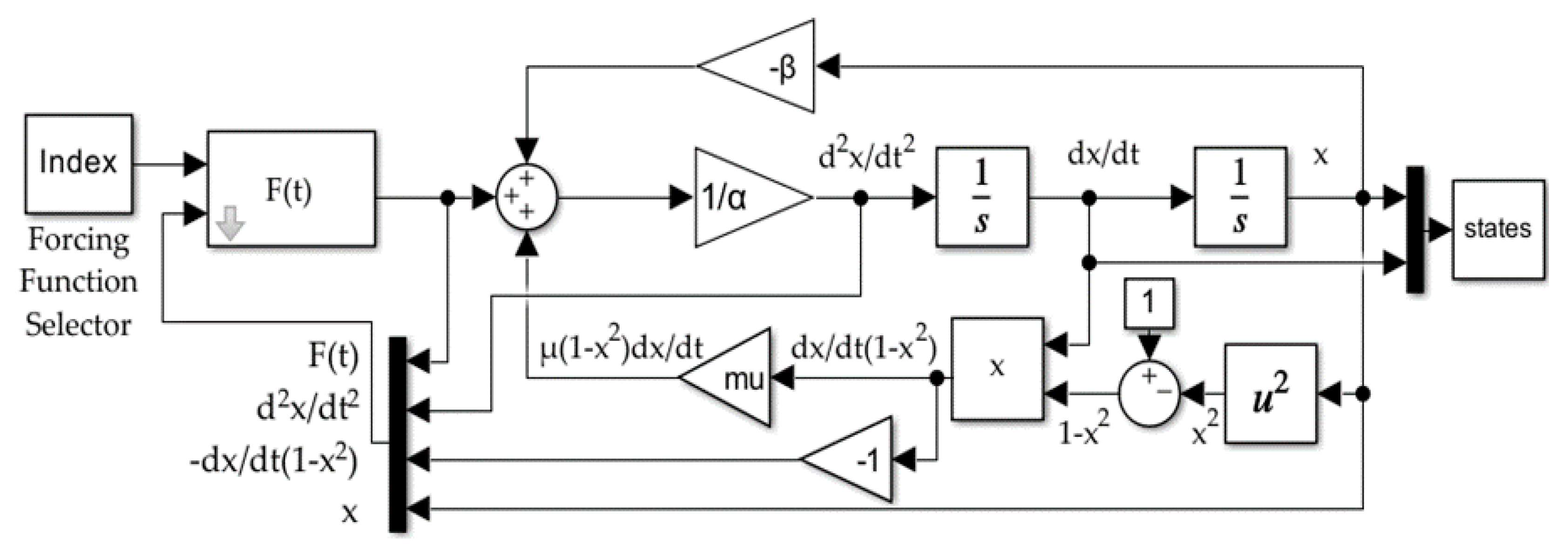
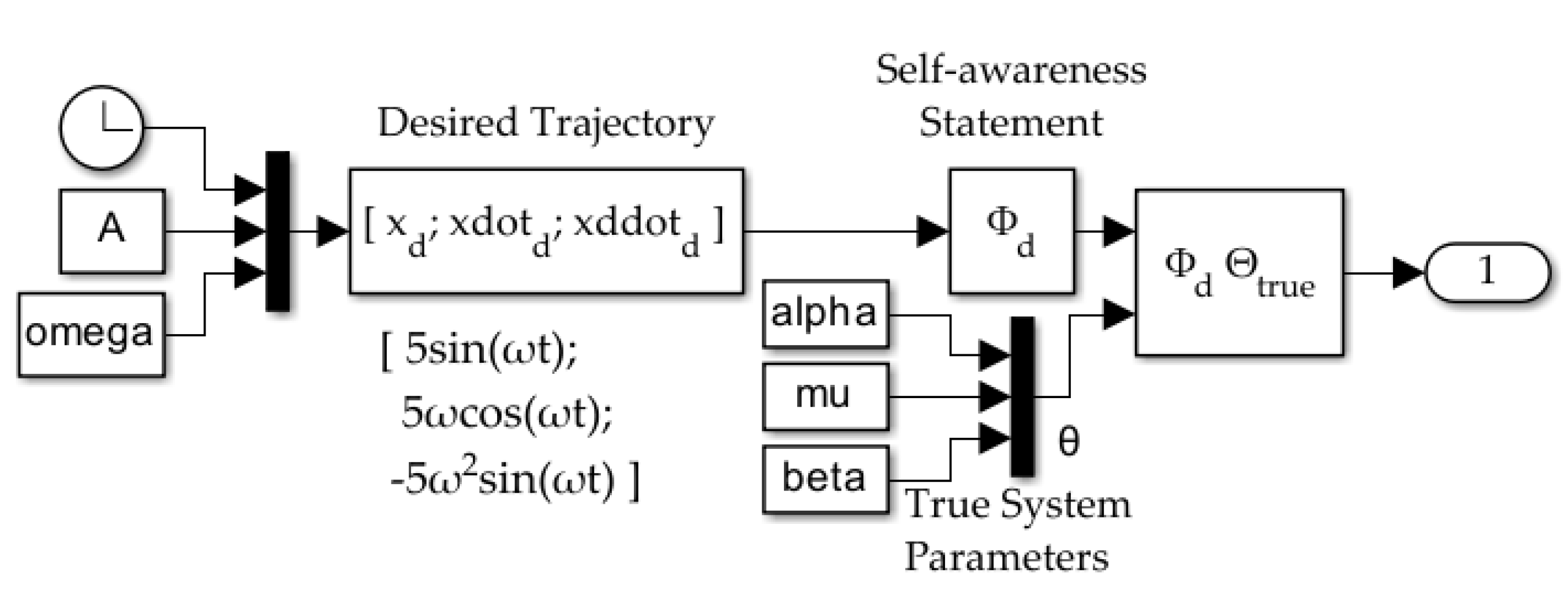
  • Using a Kalman filter for online estimation in a deterministic AI architecture exhibited worse performance than the Cooper–Heidlauf baseline [10]. Both recursive least squares with exponential forgetting and least mean squares performed better than baseline. Figure 4, Figure 5 and Figure 6 show the implementation of the forced van der Pol oscillator simulation in SIMULINK® with modular forcing function components. These figures in conjunction with MATLAB® code in the Appendix A facilitate extension of results.
2.
An optimal approach to online estimation for deterministic artificial intelligence may involve using more than one algorithm. The authors found that one algorithm may exhibit superior performance when the error between predicted chaotic trajectories and observed trajectories is greatest, while another may have lower error when the system approaches the limit cycle, or steady state. The authors propose this as a direction for future research.

2. Materials and Methods
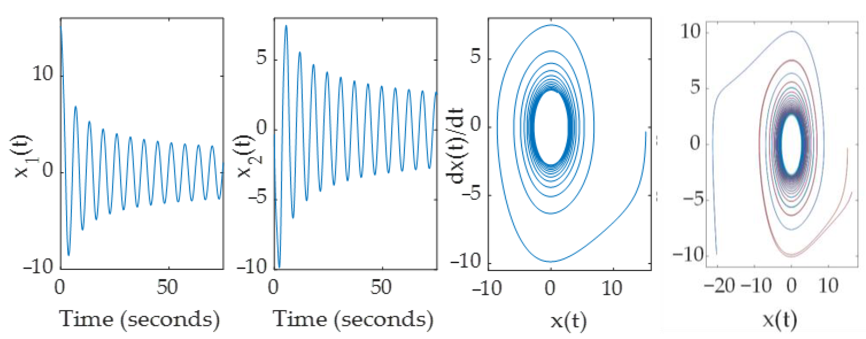
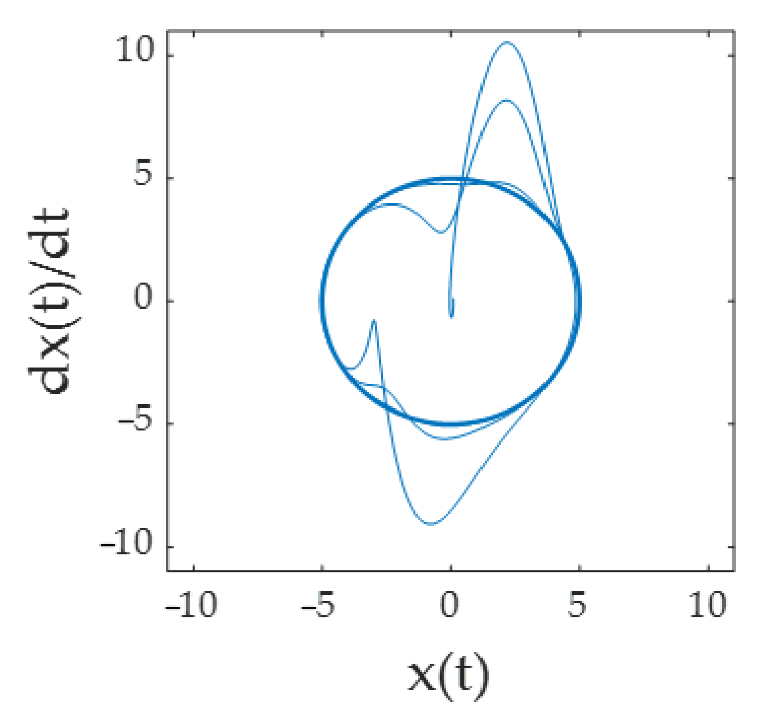
The van der Pol chaotic oscillator is defined by Equation (1):
F t = α x + μ 1 x 2 x ˙ + β x ¨
where F t is the forcing function and α , μ , and β define the system parameters, collectively referred to as θ . With deterministic artificial intelligence, the system parameters are estimated at each time step. Figure 4 is a SIMULINK® model that represents the system.
Online estimation methods analyzed in this paper require two inputs: the regressors Φ t r u e observed from the system and F t from the previous time step, F t 1 . We define the regressors as:
Φ t r u e = x 1 x 2 x ˙ x ¨
Given system inputs Φ t r u e and F t 1 , the estimator performs regression to calculate the estimated system parameters, θ ^ . These are used in conjunction with self-awareness statements to calculate F t .
Self-awareness statements are formulated using desired trajectory x d x ˙ d x ¨ d :
Φ d = x d 1 x 2 x ˙ d x ¨ d
and represent the known physics of the van der Pol system. All together, we have Equation (4):
F t = Φ d θ ^ = x d 1 x 2 x ˙ d x ¨ d x d x ˙ d x ¨ d
See Figure 5 and Figure 6 for the SIMULINK® architectures of the forcing function with feedforward only and feedforward with deterministic artificial intelligence.

3. Results

We used the Runge-Kutta MATLAB® 2022b solver in SIMULINK® with a step size of 0.01 and a simulation time of 100 s to run the model in Figure 4 given different forcing functions:
  • Unforced
  • Uniform noise
  • Sine wave
  • Feedforward
  • Deterministic artificial intelligence (DAI)—Kalman filter estimator
  • Deterministic artificial intelligence (DAI)—recursive least squares with exponential forgetting estimator.
  • Deterministic artificial intelligence (DAI)—normalized gradient least mean squares estimator
For the deterministic artificial intelligence methods, we initialized θ ^ ( α , μ , and β ) as 0.1; the ground truth value was θ = 5 1 1 . Despite the inaccuracy of the initial estimates, all deterministic artificial intelligence methods succeeded in iteratively estimating the truth values, with θ ^ converging to θ .
We analyzed the error between the trajectory of the responder van der Pol oscillator and the desired trajectory, a circle of radius 5. Code used to generate results and figures is included in Appendix A. The first three methods did not employ feedforward or deterministic artificial intelligence feedback. Both the unforced oscillator and the uniform noise forced oscillator exhibited the chaotic trajectory of characteristic of damped van der Pol oscillators, visualized at the center of Figure 7. The sine wave forced the responder oscillator to deviate from the typical van der Pol trajectory, but the resulting trajectory was chaotic. These results are shown in Table 1 and Table 2 and plotted in Figure 8.
Method 4, feedforward using the drive-response methodology in [10], successfully forced the responder oscillator to follow the target trajectory. Methods 5–7 built upon method 4, adding deterministic artificial intelligence feedback as described in [16] to estimate and learn the system parameters.

4. Discussion

A van der Pol oscillator subtends toward a limit cycle, an invariant set determined by the initial conditions. This occurs when both sides of Equation (1) are equal, or:
α x + μ 1 x 2 x ˙ + β x ¨ F t = 0
In other words, the oscillator will, after some time, converge to a fixed trajectory. The goal of [10] was to command a van der Pol oscillator such that, no matter the initial conditions, it would asymptotically approach the same limit cycle. Smeresky and Rizzo went a step further in [16] by showing that deterministic artificial intelligence can improve the ability of the forcing function, F t , to force the responder oscillator to follow a desired trajectory.
We build upon the results of [16] by comparing three different deterministic artificial intelligence system parameter estimators: a Kalman filter, recursive least squares with exponential forgetting (RLS-EF), and normalized gradient least mean squares (NLMS). We additionally compared these methods to forcing functions that do not use deterministic artificial intelligence, such a uniform noise, a sine wave, and the feedforward function in [10].
For all methods with feedforward (methods 4–7), the responder van der Pol oscillator had significant error in the beginning that decreased as the oscillator stabilized to the desired trajectory. This error approached an asymptote around zero.
Over the length of the entire simulation, 10,000 time-steps for 100 s at a sample time of 0.01, the different deterministic artificial intelligence estimator that had the lowest mean absolute error (MAE) was recursive least squares with exponential forgetting, with a 2.41% and 2.01% reduction in mean absolute error for x and x ˙ , respectively, compared to feedforward alone. See the first two results columns of Table 3 for percent improvement. We found that different deterministic artificial intelligence with the Kalman filter and normalized gradient least mean squares had worse performance than feedforward alone. These results suggested that the Kalman filter and normalized gradient least mean squares estimators should be avoided in favor of recursive least squares with exponential forgetting.
However, we noticed that deterministic artificial intelligence using the normalized gradient least mean squares estimator exhibited decreased mean absolute error as the system approached the limit cycle. See the last two results columns of Table 3 for percent improvement after t = 1000. Different deterministic artificial intelligence with normalized gradient least mean squares had 48.7% and 19.3% less mean absolute error for x and x ˙ , respectively, compared to feedforward alone, and exhibited a 47.7% and 17.7% reduction in mean absolute error for x and x ˙ compared to deterministic artificial intelligence with recursive least squares with exponential forgetting.

5. Conclusions

Simulation experiments indicate the recursive least squares with exponential forgetting algorithm for parameter estimation is relatively superior for the first 1000 time-steps of the simulation, after which normalized gradient least mean squares exhibits superior performance. One algorithm may be preferable over the other depending on the intended application. For instance, recursive least squares with exponential forgetting having relatively minimal error when the system is far from the limit cycle could indicate that the algorithm is better suited for systems where frequent external disturbances are expected.

Future Research

As a next step for future research, both recursive least squares with exponential forgetting and normalized least mean squares techniques could be used together, with the algorithm using recursive least squares with exponential forgetting for the first t time steps to estimate system parameters θ and then switching over to normalized gradient least mean squares once the system has found stability. Another research opportunity would be adding logic for the model to switch between different estimation methods when an external disturbance to the system is introduced.
More broadly, the use of hierarchical reinforcement learning for switching between estimation algorithms could be explored. Reinforcement learning involves training an agent to learn a policy in an environment, most often a simulation. The agent takes actions in the environment and receives rewards (or punishments) based on the outcome. The agent’s policy is optimized to maximize cumulative rewards [17,18].
Hierarchical reinforcement learning involves decomposing a long-horizon task into subtasks. The higher-level policy will learn to perform a task by orchestrating lower-level policies to execute the subtasks. For instance, we can consider the task of driving an autonomous car to a store. The task can be broken into different subtasks, such as drive in the lines, signal with the blinkers, and pull into the parking lot. The high-level policy would execute the principal task by breaking it down into smaller tasks and orchestrating lower-level policies to complete them [17,18].
An interesting area of future research could leverage the overall concept of hierarchical reinforcement learning for online estimation to improve deterministic artificial intelligence performance. An agent would train a high-level policy to drive the system. Its goal would be minimizing error between the predicted and actual van der Pol trajectory in a simulation. The lower-level policies of the agent would, in this case, be the different online estimation methods, such as recursive least squares with exponential forgetting and normalized least mean squares. These methods would comprise a policy bank, or zoo, that the high-level policy could call upon to perform online estimation. The authors hypothesize that the high-level policy would learn a novel algorithm for optimal switching between online estimation methods. In this future research, additional online estimation methods could be explored and added to the lower-level policy bank.
Additionally, instead of using online estimation algorithms, such as recursive least squares with exponential forgetting, as low-level policies for the hierarchical reinforcement learning algorithm, low-level policies could instead be learned through reinforcement learning. The authors would find the behavior of such trained policies of great interest. Fawzi et al. show in [26] how reinforcement learning can independently discover optimal algorithms for tasks such as matrix multiplication. The reinforcement learning algorithms in this case discovered improvements on state-of-the-art algorithms such as Strassen’s two-level algorithm, which has been recognized as the optimal algorithm for multiplication of 4 × 4 matrices for the past 50 years [26]. Future research into this domain may discover a new state-of-the-art algorithm for adaptive control, which may produce even better results within the deterministic AI framework outlined in the body of this work. Such an algorithm may have more general applicability to adaptive control theory.
A final future direction may be meta-learning, where a controller studies a related set of problems and generalizes to efficiently solve novel, similar problems. Systems that have well-understood dynamics, such as the van der Pol oscillator (see Equation (3)) are good targets for meta-learning. Ref. [27] outlines a methodology for meta-learning through reinforcement learning. Model-based information, such as self-awareness statements, are used during training, but are unavailable during execution. Consequently, a generalized policy is learned that can function in different stochastic environments. One potential benefit of this is that the model may be resistant to external interference.

Author Contributions

Conceptualization, L.R. and T.S.; methodology, L.R.; software, L.R.; validation, L.R. and T.S.; formal analysis, L.R.; investigation, L.R.; resources, L.R. and T.S.; data curation, T.S.; writing—original draft preparation, L.R. and T.S.; writing—review and editing, L.R. and T.S.; visualization, L.R.; supervision, T.S.; project administration, T.S. All authors have read and agreed to the published version of the manuscript.

Funding

This research received no external funding.

Data Availability Statement

No new data were created or analyzed in this study. Data sharing is not applicable to this article.

Conflicts of Interest

The authors declare no conflict of interest.

Appendix A

MATLAB® Code:
%%
clear all; close all; clc;
headless = 1;
RngSeed = 1;
% Oscillator Parameters
alpha = 5;
mu = 1;
beta = 1;
% RLS Parameters
rls_sample_time = 0.01;
alpha_i = 0.1;
mu_i = 0.1;
beta_i = 0.1;
% Desired Trajectory Parameters
A = 5;
omega = 1;
SampleTime = 0.01;
% Initial Conditions
x0 = 1;
v0 = 1;
%%
figure(1);
hold on;
errors = [];
errors2 = [];
episodes = 6001;
forgetting_factor = 1;
noise_covariance = 80;
adaption_gain = 0.9277;
grab_index = 1000;
for Index = 1:1:3
sim(‘SimVanDerPol’);
errors = [errors; mean(abs(states–desiredstates(1:2,:)’))]
errors2 = [errors2; mean(abs(states(grab_index:end,:)–desiredstates(1:2,grab_index:end)’))]
figure(1);
plot(states(:,1), states(:,2),’:’, ‘Linewidth’,2);hold on;
end
for Index = 4:1:7
sim(‘SimVanDerPol’);
errors = [errors; mean(abs(states–desiredstates(1:2,:)’))]
errors2 = [errors2; mean(abs(states(grab_index:end,:)–desiredstates(1:2,grab_index:end)’))]
figure(1);
plot(states(:,1), states(:,2),’:’, ‘Linewidth’,2);hold on;
figure(2);
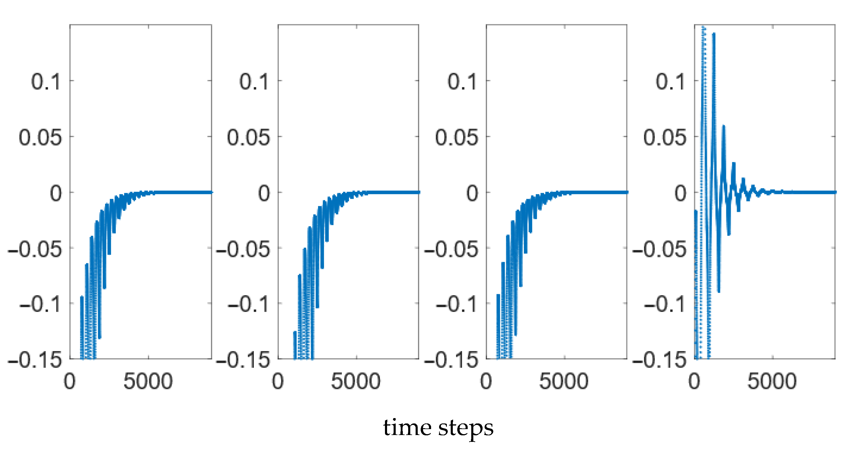
subplot(1,4,Index-3);plot(states(grab_index:end,1)–desiredstates(1,grab_index:end)’);axis([0,length(desiredstates(1,grab_index:end)),-0.025,0.025]);
end
figure(1);
plot(desiredstates(1,:), desiredstates(2,:),’:’, ‘Linewidth’,1, ‘Color’, ‘red’);hold off;
legend(“Unforced”, “Random Noise”, “Sine Wave”, “Feedforward”, “RLS Kalman”, “RLS-EF”, “Norm’d LMS”, “Goal”,’fontname’,’Palatino’, ‘fontsize’,22,’NumColumns’,2,’Location’,’northeast’,’Orientation’,’horizontal’);
set(gca,’fontname’,’Palatino’, ‘fontsize’,26);
axis([-9,9,-9,9]);
xlabel(“x(t)”,’fontname’,’Palatino’, ‘fontsize’,32); ylabel(“dx(t)/dt”,’fontname’,’Palatino’, ‘fontsize’,26);
figure(3);
subplot(1,2,1);plot(abs(errors(:,1)));
subplot(1,2,2);plot(abs(errors(:,2)));

References

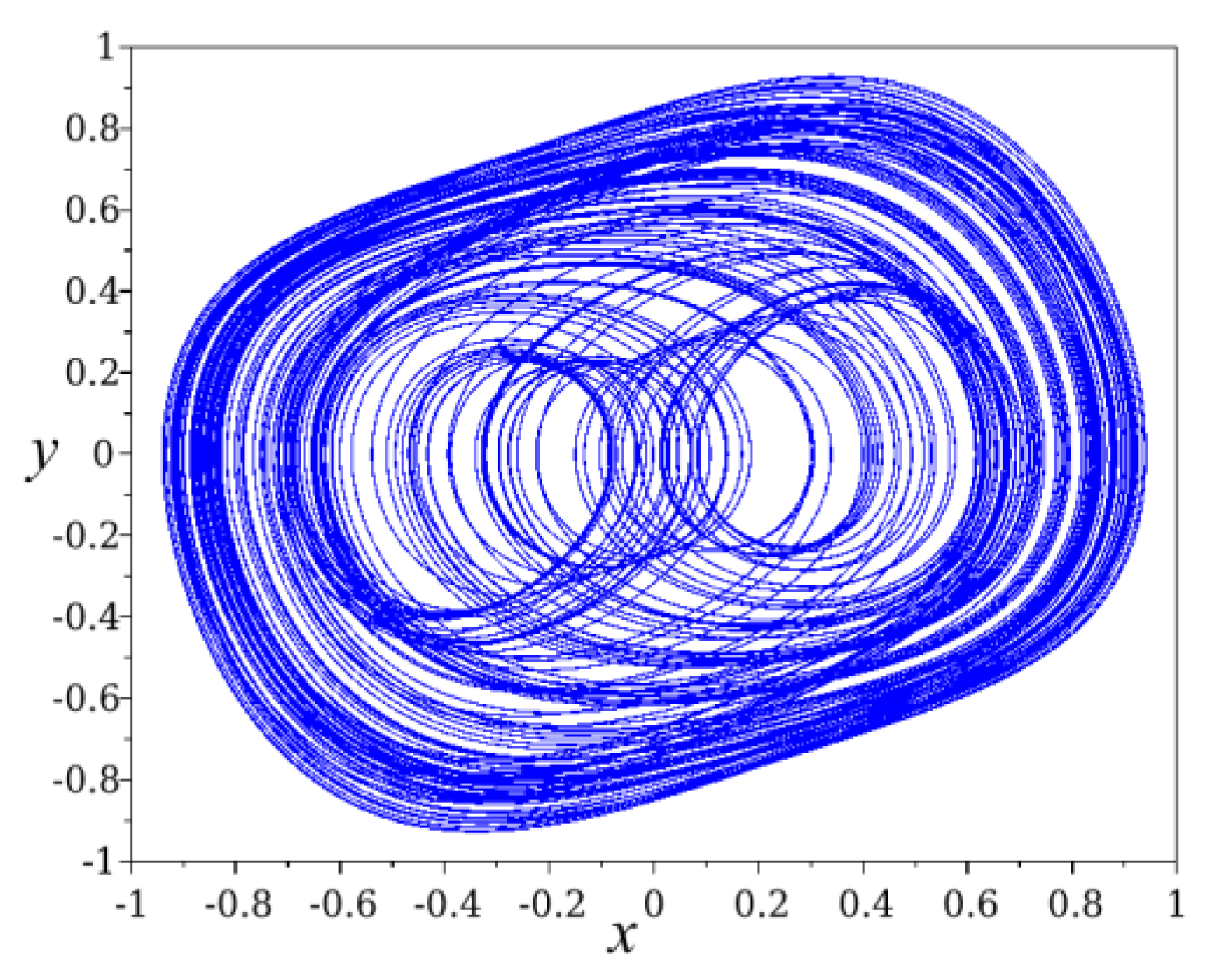
  1. File: Strange Attractor of van der Pol and Duffing Mixed Type Equation.svg. Available online: https://commons.wikimedia.org/wiki/File:Strange_attractor_of_van_der_Pol_and_Duffing_mixed_type_equation.svg (accessed on 27 February 2023).
  2. CC0 1.0 Universal (CC0 1.0) Public Domain Dedication. Available online: https://creativecommons.org/publicdomain/zero/1.0/deed.en (accessed on 27 February 2023).
  3. Cassady, J.; Maliga, K.; Overton, S.; Martin, T.; Sanders, S.; Joyner, C.; Kokam, T.; Tantardini, M. Next Steps in the Evolvable Path to Mars. In Proceedings of the International Astronautical Congress, Jerusalem, Israel, 12–16 October 2015. [Google Scholar]
  4. Song, Y.; Li, Y.; Li, C. Ott-Grebogi-Yorke controller design based on feedback control. In Proceedings of the 2011 International Conference on Electrical and Control Engineering, Yichang, China, 24 October 2011; pp. 4846–4849. [Google Scholar]
  5. Pyragas, K. Continuous control of chaos by self-controlling feedback. Phys. Lett. A 1992, 170, 421–428. [Google Scholar] [CrossRef]
  6. Slotine, J.; Li, W. Applied Nonlinear Control; Prentice-Hall, Inc.: Englewood Cliffs, NJ, USA, 1991; pp. 392–436. [Google Scholar]
  7. Osburn, J.; Whitaker, H.; Kezer, A. New Developments in the Design of Model Reference Adaptive Control Systems; Institute of the Aerospace Sciences: Reston, VA, USA, 1961; Volume 61. [Google Scholar]
  8. Fossen, T. Handbook of Marine Craft Hydrodynamics and Motion Control, 2nd ed.; John Wiley & Sons Inc.: Hoboken, NJ, USA, 2021. [Google Scholar]
  9. Fossen, T. Guidance and Control of Ocean Vehicles; John Wiley & Sons Inc.: Chichester, UK, 1994. [Google Scholar]
  10. Cooper, M.; Heidlauf, P.; Sands, T. Controlling Chaos—Forced van der Pol Equation. Mathematics 2017, 5, 70. [Google Scholar] [CrossRef] [Green Version]
  11. van der Pol, B. A note on the relation of the audibility factor of a shunted telephone to the antenna circuit as used in the reception of wireless signals. Philos. Mag. 1917, 34, 184–188. [Google Scholar] [CrossRef] [Green Version]
  12. van der Pol, B. On “relaxation-oscillations”. Lond. Edinb. Dublin Philos. Mag. J. Sci. 1926, 2, 978–992. [Google Scholar] [CrossRef]
  13. van der Pol, B.; van der Mark, J. Frequency Demultiplication. Nature 1927, 120, 363–364. [Google Scholar] [CrossRef]
  14. van der Pol, B.; van der Mark, J. The heartbeat considered as a relaxation-oscillation, and an electrical model of the heart. Philos. Mag. 1929, 6, 673–675. [Google Scholar] [CrossRef]
  15. van der Pol, B. The nonlinear theory of electric oscillations. Proc. IRE 1934, 22, 1051–1086. [Google Scholar] [CrossRef]
  16. Smeresky, B.; Rizzo, A.; Sands, T. Optimal Learning and Self-Awareness Versus PDI. Algorithms 2020, 13, 23. [Google Scholar] [CrossRef] [Green Version]
  17. Zhai, H.; Sands, T. Controlling Chaos in Van Der Pol Dynamics Using Signal-Encoded Deep Learning. Mathematics 2022, 10, 453. [Google Scholar] [CrossRef]
  18. Zhai, H.; Sands, T. Comparison of Deep Learning and Deterministic Algorithms for Control Modeling. Sensors 2022, 22, 6362. [Google Scholar] [CrossRef] [PubMed]
  19. Plackett, R. Some Theorems in Least Squares. Biometrika 1950, 37, 149–157. [Google Scholar] [CrossRef] [PubMed]
  20. Astrom, K.; Wittenmark, B. Adaptive Control, 2nd ed.; Addison Wesley Longman: Boston, MA, USA, 1995. [Google Scholar]
  21. Patra, A.; Unbehauen, H. Nonlinear modeling and identification. In Proceedings of the IEEE/SMC’93 Conference System Engineering in Service of Humans, Le Touquet, France, 17–20 October 1993. [Google Scholar]
  22. Martinek, R.; Kahankova, R.; Nedoma, J.; Fajkus, M.; Skacel, M. Comparison of the LMS, NLMS, RLS, and QR-RLS algorithms for vehicle noise suppression. In Proceedings of the 10th International Conference on Computer Modeling and Simulation, Sydney, Australia, 8–10 January 2018; pp. 23–27. [Google Scholar]
  23. Welch, G.; Bishop, G. An introduction to the Kalman filter. In UNC Chapel Hill, Department of Computer Science Technical Report, 95-041; University of North Carolina at Chapel Hill: Chapel Hill, NC, USA, 1995. [Google Scholar]
  24. Ramirez, P.S. The Least-Mean-Square (LMS) Algorithm. In Adaptive Filtering; The Kluwer International Series in Engineering and Computer Science, 694; Springer: Boston, MA, USA, 2002. [Google Scholar]
  25. Pateria, S.; Subagdja, B.; Tan, A.H.; Quek, C. Hierarchical Reinforcement Learning: A Comprehensive Survey. ACM Comput. Surv. 2021, 54, 109. [Google Scholar] [CrossRef]
  26. Fawzi, A.; Balog, M.; Huang, A.; Hubert, T.; Romera-Paredes, B.; Barekatain, M.; Novikov, A.; RRuiz, F.J.; Schrittwieser, J.; Swirszcz, G.; et al. Discovering faster matrix multiplication algorithms with reinforcement learning. Nature 2022, 610, 47–53. [Google Scholar] [CrossRef] [PubMed]
  27. McClement, D.G.; Lawrence, N.P.; Forbes, M.G.; Loewen, P.D.; Backström, J.U.; Gopaluni, R.B. Meta-Reinforcement Learning for Adaptive Control of Second Order Systems. In Proceedings of the 2022 IEEE International Symposium on Advanced Control of Industrial Processes (AdCONIP), Vancouver, BC, Canada, 7–9 August 2022; pp. 78–83. [Google Scholar]
Figure 1. The strange attractor of van der Pol and Duffing mixed type equation [1]. Image credit Yapparina, CC0, via Wiki-media Commons used in accordance with image use policy [2].
Dynamics 03 00012 g001
Figure 2. Left: The response and phase plot of a non-forced, dampened van der Pol oscillator for one set of initial conditions. Right: The phase plot for multiple initial conditions; note the divergence of trajectories characteristic of a chaotic system.
Dynamics 03 00012 g002
Figure 3. The van der Pol response oscillator is forced to follow a prescribed circular trajectory. Error between the response oscillator trajectory and the target trajectory asymptotically approaches zero.
Dynamics 03 00012 g003
Figure 4. The forcing function block, F t , drives the van der Pol oscillator. State information is passed into the forcing function block, to be used by deterministic artificial intelligence to estimate the system parameters.
Dynamics 03 00012 g004
Figure 5. The forcing function block, F t , with feedforward only.
Dynamics 03 00012 g005
Figure 6. The forcing function block, F t , adding DAI feedback as derived in [10,16]. In the depicted simulation, the Estimator block utilizes one of three methods to calculate θ ^ : Kalman filter, recursive least squares with exponential forgetting, and normalized gradient least mean squares.
Dynamics 03 00012 g006
Figure 7. The van der Pol response oscillator trajectory plotted against the target trajectory, a circle of radius 5, for each of the forcing functions. Methods 4–7 successfully force the response oscillator to follow the target trajectory.
Dynamics 03 00012 g007
Figure 8. Error of x calculated over time for methods 4–7, in order. Note that the error curve of method 7, normalized gradient least mean squares, is distinct from the others. MAE is used in assessing model performance to handle both positive and negative error swings.
Dynamics 03 00012 g008
Table 1. Mean absolute error (MAE) for the entire trajectory.
Method M A E   x Method M A E   x ˙
13.323413.2031
23.333423.2110
33.984333.9275
40.209140.2284
50.497550.3927
60.204160.2237
70.308970.2877
Table 2. Mean absolute error (MAE) when excluding the first 10% of the trajectory.
Method M A E   x Method M A E   x ˙
13.321813.1891
23.326223.1941
34.015033.9487
40.064240.0743
50.122050.1379
60.062960.0728
70.032970.0599
Table 3. Performance comparison. Percent mean absolute error improvement calculated between the deterministic artificial intelligence methods and method 4, feedforward only. The best result in each column is highlighted.
MethodStarting at t = 1
MAE x
(% ± Rel. Method 4)
Starting at t = 1
MAE x ˙
(% ± Rel. Method 4)
Starting at t = 1000
MAE x
(% ± Rel. Method 4)
Starting at t = 1000
MAE x ˙
(% ± Rel. Method 4)
Feedforward Only (Method 4)
DAI with Kalman filter (Method 5)−137.86−71.93−90.1−85.7
DAI with RLS-EF (Method 6)2.412.041.971.93
DAI with NLMS (Method 7)−47.69−25.9848.7019.32
Disclaimer/Publisher’s Note: The statements, opinions and data contained in all publications are solely those of the individual author(s) and contributor(s) and not of MDPI and/or the editor(s). MDPI and/or the editor(s) disclaim responsibility for any injury to people or property resulting from any ideas, methods, instructions or products referred to in the content.

