Article

Global Sensitivity Analysis and Uncertainty Quantification for Simulated Atrial Electrocardiograms

1
Physikalisch-Technische Bundesanstalt, Abbestraße 2, 10587 Berlin, Germany
2
Institute of Biomedical Engineering, Karlsruhe Institute of Technology (KIT), Kaiserstraße 12, 76131 Karlsruhe, Germany
3
Institute of Theoretical Physics, Technische Universität Berlin, Straße des 17. Juni 135, 10623 Berlin, Germany
*
Author to whom correspondence should be addressed.
Metrology 2023, 3(1), 1-28; https://doi.org/10.3390/metrology3010001
Submission received: 15 September 2022 / Revised: 16 December 2022 / Accepted: 19 December 2022 / Published: 26 December 2022
(This article belongs to the Special Issue Virtual Measuring Systems and Digital Twins)

Abstract

:
The numerical modeling of cardiac electrophysiology has reached a mature and advanced state that allows for quantitative modeling of many clinically relevant processes. As a result, complex computational tasks such as the creation of a variety of electrocardiograms (ECGs) from virtual cohorts of models representing biological variation are within reach. This requires a correct representation of the variability of a population by suitable distributions of a number of input parameters. Hence, the assessment of the dependence and variation of model outputs by sensitivity analysis and uncertainty quantification become crucial. Since the standard metrological approach of using Monte–Carlo simulations is computationally prohibitive, we use a nonintrusive polynomial chaos-based approximation of the forward model used for obtaining the atrial contribution to a realistic electrocardiogram. The surrogate increases the speed of computations for varying parameters by orders of magnitude and thereby greatly enhances the versatility of uncertainty quantification. It further allows for the quantification of parameter influences via Sobol indices for the time series of 12 lead ECGs and provides bounds for the accuracy of the obtained sensitivities derived from an estimation of the surrogate approximation error. Thus, it is capable of supporting and improving the creation of synthetic databases of ECGs from a virtual cohort mapping a representative sample of the human population based on physiologically and anatomically realistic three-dimensional models.

1. Introduction

The modeling of cardiac electrophysiology has initially focused on the qualitative understanding of normal cardiac rhythm and pathologies such as atrial and ventricular fibrillation or T-wave alternans by combining numerical simulations and approaches from nonlinear dynamics. Many underlying mechanisms of arrhythmias are by now well understood, oftentimes by considering simplified cellular models in one or two spatial dimensions or idealized geometries [1,2,3,4,5]. Recent years have seen in contrast a clear evolution towards quantitative models. To achieve this, improved and more detailed physiological models are being solved on realistic anatomical models, obtained, e.g., from magnetic resonance imaging [6]. This enables the reproduction of clinically relevant aspects such as cardiac activation maps or even electrocardiograms [7,8]. Based on the optimistic vision of a digital twinning of cardiac function and dynamics [9,10,11,12], complex computational tasks such as the development of personalized, patient-specific models from experimental recordings or the creation of virtual cohorts of models, statistically representing a large realistic sample of a population [13,14], are realized.
In this paper, we deal specifically with the metrological aspects of creating a database of realistic synthetic ECGs obtained from simulation of a cohort of models. The goal is to reproduce the features of ECGs in recently published large clinical data bases such as PTB-XL [15] and Chapman [16]. Such databases are important for developing and benchmarking machine learning algorithms for automated diagnostics of ECGs, see e.g., [17,18,19]. This endeavor requires a correct representation of the anatomical and physiological variability of a population, which can be achieved by variations of model geometries and a considerable number of functional model input parameters. For that, sensitivity analysis (SA) and uncertainty quantification (UQ), i.e., the assessment of the variation of models outputs in relation to the variation of model input parameters, have to be applied to the complex computational models developed for faithful simulations of realistic ECGs mentioned above. UQ for models of cardiac dynamics has already attracted a lot of interest that is documented by white papers such as [20], many dedicated journal and proceedings articles [21,22,23,24,25,26,27,28,29,30,31,32,33], as well as various special issues of scientific journals in recent years, see, e.g., [34,35]. In this work, we introduce and illustrate an approach for SA and UQ of the atrial contribution of virtual electrocardiogram data. Synthetic ECGs are generated by solving partial differential equations (PDE) of the electrical activity of virtual hearts, residing inside realistic torso models [10,36]. At the surface of the torso models, virtual electrodes measure the electrical potential and thereby construct the so-called ECG leads by calculating the potential difference between 12 different combinations of electrodes. This resembles the physical measurement of an electrocardiogram in live patients, where a physician places the electrodes in a fixed pattern on a patient’s body. The so-called 12-lead ECG is a standard monitoring scheme to observe a patient’s heart activity in the short and long-term, as well as to identify specific pathologies such as arrhythmias [37,38,39,40]. These can be linked to several cardiovascular diseases (CVDs), which are among the most common causes for mortality world wide, i.e., contributing more premature deaths by non-communicable diseases than cancer worldwide, according to the WHO world health statistics 2019. The in-depth simulation approach to virtually measure ECG data comes with many challenges of numerical and medical nature but exhibits clear advantages over purely signal-driven or data-driven approaches. Most prominently, the complete modeling from the cellular level upwards facilitates the understanding of sensitivity aspects of the involved parameters on all levels up to the ready electrocardiogram. That way, it becomes possible to distinguish between different pathologies in the patient from non-pathological variances such as normal geometrical variability or measurement uncertainties, most prominently from the application of the electrodes on the patient’s torso.
The challenge to compute sensitivities and quantify uncertainties in the detailed atrial models stems from the computation expense. Standard approaches for nonlinear models frequently used in metrology are Monte–Carlo simulations as outlined, e.g., in the GUM supplement 1 [41]. However, they are computationally prohibitive in our setting since they require a large number of repetitions of expensive three-dimensional simulations with varying input parameters. Following earlier good practice in metrology guidance [42], we instead use an approach based on the creation of a surrogate model, i.e., a mathematical model that is built from simulations of the original model and subsequently allows simulations with much lower computational cost. More importantly, surrogate models are also a central topic in the recently emerged applied mathematical field of UQ [43,44,45] and have found already widespread application mostly based on the polynomial chaos expansion (PCE) in a number of traditional metrological applications ranging from optics [46,47] to thermophysics [48] and fluid dynamics [49]. Whereas these metrological examples above typical dealt with UQ of a single or a few stationary measurement quantities, here, we need to compute the uncertainty for several dynamically evolving timeseries. For that, we use a nonintrusive polynomial chaos-based approximation of the forward model and demonstrate that it is well suited to describe the signal variance of an explicitly simulated cohort of P-waves, i.e., the atrial contribution to the electrocardiogram. This variance-based method allows for a global sensitivity analysis and determination of Sobol coefficients at no additional computational overhead [50]. In addition, the resulting surrogate model enables UQ since the distribution of outputs can be computed for a given input distribution with reasonable computational effort. Hence, the use of a polynomial chaos surrogate allows for quantifying both parameter influences and surrogate approximation uncertainties for the atrial contribution to the time series characterizing a 12 lead ECG.
The paper is organized as follows: The detailed computational model is introduced in Section 2.1. It starts from the ion channels in the cell membranes of the myocardium, integrated these cellular models for tissue level descriptions and uses MRI scans of real atria to generate anatomically accurate geometries on which the electrophysiological model runs. The atria mesh is placed inside a realistic torso model and virtual electrodes are placed onto the torso surface, recording the differences in the electrical potential to calculate the 12 leads of the ECG. After that, in Section 2.2, we give an introduction on variance-based SA by means of Sobol indices. The generalized PCE scheme is outlined in Section 2.3, as well as the specific numerical implementation of the PyThia software used for analyzing the datasets. The generation of the specific datasets used is described in Section 2.4. The results are divided into three sections. First, we investigate in detail how well the PCE surrogates represent the underlying sampled data by addressing the surrogate error convergence with respect to the used maximal polynomial order and with respect to the number of samples used to create a surrogate, cf. Section 3.1. After that, the SA is performed first on the whole, time-dependent signal and then also by integrating the Sobol indices of a complete lead, cf. Section 3.2. In the last part of the result, the created surrogate model is used to enhance the UQ and the strengths of the PCE method are demonstrated, cf. Section 3.3. We finish with a discussion of the findings in Section 4 and conclusions drawn from the analysis in Section 5.

2. Materials and Methods

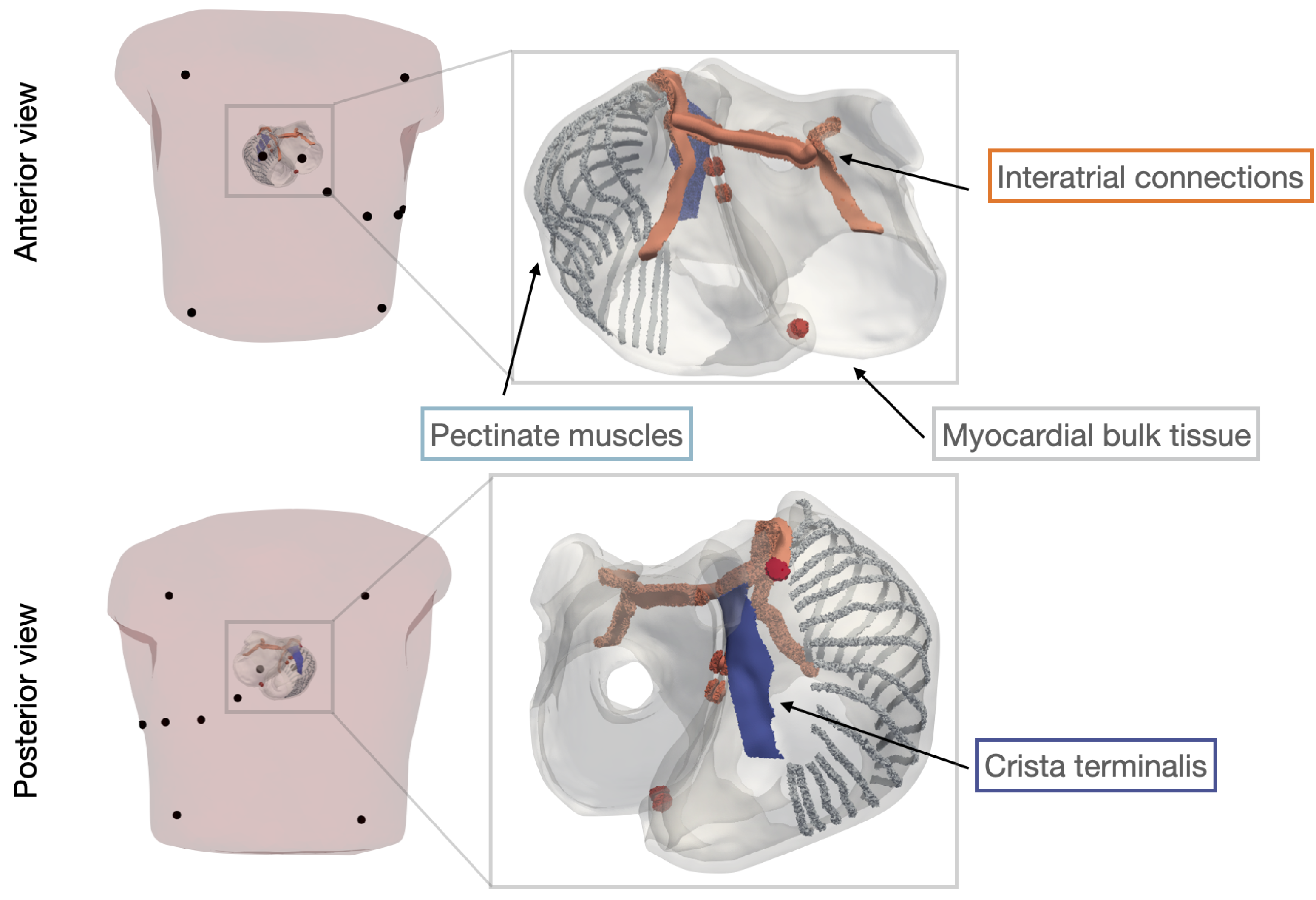
2.1. The Atrial Model

A patient-specific tetrahedral atrial model with an average edge length of 1.64 mm was built based on the descriptions in [51]. The algorithms described by Azzolin et al. [11] were applied to the atrial geometry to automatically augment the model with a homogeneous wall thickness of 3 mm, tags for anatomical structures, interatrial connections and myocardial fiber orientation in a rule-based fashion. Based on the material tags, the atria were subdivided into 4 tissue regions visualized in Figure 1 with different conduction properties assigned to them. Transversal conduction velocity was set to 0.591 m/s and 0.461 m/s for crista terminalis and the pectinate muscles, respectively. For the myocardial bulk tissue and the interatrial connections, transversal conduction velocity was varied in the intervals listed in Table 1. Anisotropy ratios describing the fraction between longitudinal and transversal conduction velocity were set to 2.09, 3.34, 2.84 and 3.78 based on the values reported in [51] for the myocardial bulk tissue, interatrial connections, crista terminalis and the pectinate muscles, respectively. The spread of the depolarization wavefront was obtained by solving the Eikonal equation by means of the Fast Iterative Method. The ionic model described by Courtemanche et al. [52] was used to compute an action potential template on a slab geometry. This action potential template was shifted in time according to the local activation times resulting from the Eikonal simulation to derive the spatio-temporal distribution of the transmembrane voltages in the atria [36].
The atrial model was placed in its associated patient-specific torso geometry obtained through tomographic image segmentation to define a reference position and orientation of the atria inside the torso volume conductor. Rotation angles and displacement parameters around and along the x-, y- and z-axis were applied to the heart geometry in the intervals defined in Table 1 to vary the heart orientation and location relative to the reference settings [14,53]. Subsequently, the boundary element method [54] was employed to solve the forward problem of electrocardiography and project the electrical dipole sources from the heart onto the body surface. For a computationally efficient calculation of the transfer matrix, downsampled surface meshes bounding the atria and the torso at a resolution of 2.9 mm and 15 mm, respectively, were generated. To avoid discontinuous wave propagation and artefacts in the body surface potentials due to the coarser mesh resolution, we applied Laplacian blurring to the source distribution on the cardiac surface as described by Schuler et al. [55]. Extracting the potentials at the standardized electrode positions yielded the P-waves of the 12-lead ECG resulting from each simulation run.
To generate the P-wave datasets characterized by a small and large variation of selected model parameters, the parameter values were sampled in the intervals listed in Table 1. We chose the CV in the fast conducting Bachmann’s bundle as the main conduction pathway between both atria and CV in right and left atrial bulk tissue accounting for a large fraction of the total myocardial tissue volume. Furthermore, location and translation of the heart within the torso were addressed as notable inter-individual variability regarding these quantities are observed and reported in previous clinical studies [53].

2.2. Global Sensitivity Analysis, Uncertainty Quantification and Sobol Indices

Sensitivity analysis is the study of how strong a given model output depends on the various input parameters or conditions. Typically, one aims to establish how sensitive the different output values or distributions vary with respect to a given variation in the model input, given by either single parameter variations or simultaneously varied sets of parameters. The valuable insights obtained that way can inform the model building process—especially in engineering models with huge parameter spaces, aimed at finely-tuned representations of an underlying ground truth known by measurements. Further, it helps in communicating the obtained modeling results by providing additional information, e.g., on the model reliability and the behavior of solution distributions in terms of propagated uncertainties. SA is a meta-analysis that treats the forward model M : X Y as a “black box” acting on the stochastic input vector X and generating the associated set of (stochastic) output values Y . The model M may consist of a single measurement or (arbitrary complex) numerical calculations, possibly involving an extensive pipeline of data generation and post-processing steps. SA is closely related to the problem of uncertainty quantification (UQ) that emphasises more the exact propagation of uncertainty through the model in the form of parameter distributions that are reflected in the distributions of model observables in order to address levels of confidence of results. In the present contribution, we analyze a nonlinear and high-dimensional modeling pipeline that involves numerically solving parametric partial differential equations describing the propagation of a heart’s electrical excitation and a subsequent virtual measurement of 12-lead ECG data, cf. Section 2.1. The model is characterized by complex behavior in a very high dimensional state space, i.e., the system behavior depends on many parameters in a non-monotonous manner, exhibits several qualitatively different regimes of solutions, it is nonlinear and hence obtained solutions cannot be linearly superposed to generate a complete description for arbitrary input parameters. Further, the sensitivity of the system output varies not only along the time-dependent 12 lead signal, but also with respect to different input parameter values, i.e., the specific position in parameter space.
For SA, there are so-called local and global approaches. The analysis of a system with a given set of input parameters X = ( x 1 , x 2 , x N ) is considered to be local at a given point in state space X ^ if the change of observables is calculated only with respect to infinitesimal input parameter variations around X ^ . In this case, it is sufficient to linearize the problem by restricting the analysis to small single parameter variations around X ^ , i.e., to calculate the local gradient by performing N additional measurements X i ^ of the system, in each shifting one of the input parameters x i by a small amount d x i . By subtracting the respective value at the reference point X ^ , one obtains the set of N different variations for the model output, which represents the local sensitivity of the system with respect to its input parameters locally at X ^ . However, here, we are interested in a global sensitivity analysis, i.e., the information concerning a model’s sensitivity on a finite domain. This approach is also necessary for UQ, because it deals with the propagation of parameter distributions, i.e., by design an extended parameter range has to be considered. Typically, x i is expected to possess known and mutually independent distributions [56]—although also first generalizations to inter-dependent input parameters exist [57]. Hence, the linear scaling of terms N for the single parameter variations is not sufficient as one has to take into account all possible parameter combinations, leading to the so-called “curse of dimensionality”, an exponential scaling for the number of terms to be considered ( 2 N ). The global SA approach delivers a more complete picture of the model behavior, better supporting the model building or calibration process. Moreover, a surrogate model constructed on a finite parameter domain enables the convenient performance of UQ by quickly sampling the surrogate model with different parameter distributions. The UQ is especially valuable in the clinical context where the different measurement uncertainties, the healthy biological variations and pathologies (i.e., the input variations) as well as typical ECG signals (the model output) are well known and documented. Hence, a given model can be compared to well-established medical data for validation and then creates additional insight because of the bottom-up connection to tissue level and even cell level parameters, underlying the numerical model.
To asses the sensitivity of a given model with respect to its input parameters X , we employ the calculation of Sobol indices (SI) based on the decomposition of output variance into the different contributions of the input parameters [58,59]. Next to the Sobol approach, also the Morris method [60] (and recent improvements for interdependent input parameters [61]) exists. In the so-called variance-based SA of calculating Sobol indices, first the model output Y = M ( X ) is generated for a set of input parameter combinations in a probabilistic manner. The output variance is then decomposed into the different proportions, in first order attributed to each input parameter individually. With increasing order, also parameter combinations (pairwise variations, triplets, etc.) are considered until all possible sets of input parameter combinations are adressed [62]. For that, M has to be an integrable function and can be orthogonally decomposed as:
M ( X ) = M 0 + Σ i M i ( x i ) + Σ i < j M i j ( x i , x j ) + + M 1 2 N ( x 1 , x 2 , x N ) ,
where M 0 is a constant, corresponding to the system output of the mean of the input parameters, i.e., the expected value of M . In increasing order, the terms of M then depend on all single parameters x i in first order, all pairs of parameters ( x i , x j ) in second order and so on until the last term M 1 2 N ( x 1 , x 2 , x N ) which represents the proportion of the model function that depends on all input parameters. Due to the orthogonality of the decomposition of Equation (1), the terms in higher order describe only the additional effect with respect to the lower-order variations, e.g., M 1 , 2 describes the second order effect of parameters x 1 and x 2 being varied simultaneously, without the effects of varying x 1 and x 2 independently ( M 1 and M 2 , respectively). We now require M to be square integrable and without loss of generality that all x i [ 0 ,   1 ] . We then integrate M 2 over [ 0 ,   1 ] N to obtain:
V ( M ) = M 2 ( X ) d X M 0 2 = Σ i M i 2 ( x i ) d x i + Σ i < j M i j 2 ( x i , x j ) d x i d x j + + M 1 2 N 2 ( x 1 , x 2 , x N ) d X = V i ( M ) + V i j ( M ) + V 1 , 2 N ( M ) ,
where the left hand side is the total variance V of the model M on [ 0 ,   1 ] N and the right hand side corresponds to the variances V i due to single parameter variations, V i j due to simultaneous variations of all parameter pairs, etc., until V 1 , 2 , . . N , the contribution added by the simultaneous variation of all input parameters simultaneously.
The Sobol indices S are then defined by the ratio of the different contributions on the right hand side and the total variance V. Hence, the first order Sobol indices S i and the second order indices S i j are defined as:
S i = V i V , S i j = V i j V
and similar up to the maximal order N. By definition, the sum of all Sobol indices is 1.

2.3. Polynomial Chaos Expansion

PCE was originally introduced in 1938 by Norbert Wiener as a means to approximate Gaussian random variables in terms of Hermite polynomials [63]. Only in recent years, fueled by the generalizations to non-Gaussian distributions (also called generalized polynomial chaos, gPCE) [64] and subsequent rigorous proofs of its L 2 convergence [65], it has been taken up in the metrology community as a means to treat the parametric uncertainty of models in a systematic way.
In PCE, the stochastic output vector Y = ( y 1 , y 2 y M ) of the model M acting on a set of N random Gaussian variables X = ( x 1 , x 2 x N ) is expanded in an infinite series [50,64] as:
Y ( x , t , X ) = i = 0 γ i ( x , t ) Ψ i ( { x n } n = 0 N ) ,
where γ i ( x , t ) are the expansion coefficients still depending on the non-stochastic variables such as a the position x in space or time t. Ψ i are the multivariate Hermite polynomials of the (normalized) independent Gaussian variables x n . In the present contribution, we consider a time-dependent output Y ( t ) described by the time-dependent γ i ( t ) at 152 discrete values of a voltage in the mV-range, measured in increments of 1 ms for a single lead. In the gPCE framework, the random input variables may have different distributions with a finite second moment and the Ψ i are generalized to be appropriate orthogonal polynomials, forming a basis of the appropriate Hilbert space. For a number of standard distributions, the associated family of polynomials is known: for the uniform distribution x i [ 1 , 1 ] , the Legendre polynomials are used, for Gamma-distributed variables on [ 0 , ] , Laguerre polynomials are associated and for Beta-distributed variables on [ 1 , 1 ] , the Jacobi polynomials [64,66] are used. In practice, the expansion (4) has to be truncated at a finite polynomial order i m a x = p , yielding the PC approximation of order p Y P C p Y . This introduces a finite truncation error for every PCE with respect to the underlying ground truth data. The total number N γ ( N , p ) of necessary coefficients γ i to be determined for the N independent input parameters scales exponentially with p as N γ = N p . Hence, in practice the PCE is constructed by restricting the maximum degree of the multivariate polynomials, cf. [50] for a complete derivation. For that, consider first the appropriate univariate polynomials P n ( X ) for each input variable x i separately. In the gPCE, the distributions of different input parameters can be chosen independently, hence, the chosen polynomials generally differ between x i . Further, consider the multi-index of natural numbers α = ( α 1 , α 2 α N ) with i = 1 M α i p . The total parameter space is spanned by a tensor product of the single parameters, hence, the complete basis for the whole set of input parameters can be obtained by multiplication:
Ψ α ( x 1 , x 2 x N ) = i = 1 M P α i ( x i )
Thereby, the number of polynomials—and with that the number of expansion coefficients—are reduced to:
N γ = ( p + N ) ! p ! N !
For the numerical estimation of the γ i , we use a non-intrusive regression method [67] that uses model evaluations of parameter sets in stochastic sampling schemes [68,69]. Apart from the truncation error, which decreases with a higher maximum polynomial order used for the surrogate, the sample-based estimation of the expansion coefficients introduces a second error. The numerical error of the regression decreases with the number of samples used and may depend on the specific distribution of samples over the input parameter interval. Both parts of the combined approximation error will be addressed in Section 3.1 separately. By defining an appropriate error measure that relies on comparing single model evaluations to the corresponding output via surrogate model and a dedicated test dataset, the accuracy of a calculated surrogate can be inferred.
For the means of SA (cf. Section 2.2), the PCE allows for a convenient calculation of Sobol indices. By rearranging the multi-index α to depend only on the respective parameters and with that the polynomials Ψ α , one finds the unique Sobol decomposition of the PC surrogate f P C [50]. The PC-based Sobol indices are then calculated with minimal computational effort by square-summing the terms of the Sobol decomposition and appropriate normalization by the total variance D P C , cf. Equation (51) in [50] and its derivation. Due to the fact that the Sobol indices become available analytically after a PCE surrogate is calculated from the model sampling procedure, it can be shown that the surrogate errors give an upper bound also for the PC-based Sobol indices. Assuming that the PC approximation Y P C p of the model function M satisfies | ( Y P C p M ) | < ϵ for some finite, positive ϵ , one finds the following upper bound for the Sobol indices [70]:
| S β S β p | < ϵ V ( M ) < ϵ V ( Y P C p ) ,
where S β are the exact Sobol indices, S β p the Sobol indices calculated from the truncated PCE with maximum order p and β a multi-index listing the set of parameters that defines each Sobol index, respectively. Note that ϵ can be estimated from the surrogate convergence described in Section 3.1 and the total variance of the PCE V a r ( Y P C p ) is easily available from the computations. By systematically calculating PCE-based surrogates with increasing p and N S , one obtains the convergence of the surrogate model towards the underlying sampling data (in the yet-to-be-specified sense, cf. Section 3.1) and thereby to illuminate the respective truncation and regression errors involved. With that, one can find the optimal surrogate model with the available computational resources, decide whether it exhibits a sufficiently small surrogate error and gain insight about how valuable additional samples (model evaluations) are for creating better surrogate models. After finding a PCE with appropriate accuracy, the Sobol indices are calculated with their uncertainty estimated by Equation (7) to perform a global SA of the model with the defined input parameter distributions and the surrogate model may be used for generating samples to perform UQ.
By choosing different input parameter distributions for a given model M, it is possible to address different modeling related questions and problems. For instance, it is possible to consider a surrogate built on the sampled parameter intervals of a known, small input uncertainty—e.g., given by measurement accuracy. The surrogate might be rather accurate and due to relatively small parameter intervals, converging with few samples. However, it is relatively specific as it addresses a narrowly defined parameter space. If one chooses wider parameter distributions, on the other hand, one learns more about the model behavior, possibly with a lower the surrogate accuracy and more samples needed for a good convergence. Then, however, it becomes possible to sample any parameter distribution from the surrogate where the support is a subspace of the one used for creating the surrogate, i.e., the created surrogate is more versatile. Also, it is possible to identify parameter regions where the output depends especially sensitive on input variations and add samples to increase the surrogate accuracy in an adaptive manner. Another possibility in models with many parameters is an analysis of many parameters with low polynomial order with the intent of creating a second surrogate afterwards only with the most influential parameters.
For the generation of PCE surrogates, we used the Python toolbox “PyThia UQ” [71], which implements a non-intrusive approach to determine gPCE expansion coefficients via a multilinear least-squares regression. Originally, it was designed for UQ of nanostructures of photolithography masks for the creation of semi-conductor structures [67]. With PyThia, it is possible to address approximately five to twelve parameters in one dataset with a reasonable number of basis polynomials per parameter. The main restrictions at this time are caused by the strongly growing memory demands in terms of both working memory and storage space as well as computation time with increasing input dimension and maximum polynomial degree p. However, with more involved schemes to reduce the number of regression parameters, the number of simultaneously varied parameters for a global SA can be increased further. Options are sparse methods, employing the tensor train format to decompose the multi-index into suitable, low-rank tensors [72] or adaptive methods to select the most important basis polynomials iteratively Next to the multi-linear regression computation, the package provides implementations of the basis polynomials and samplers for the uniform, Gauss, Gamma and Beta distributions, as well as for the calculation of the necessary weights for the regression. From this set of univariate distributions, the multivariate distribution of the input variability of the chosen problem is defined and the complete set of basis polynomials in the gPCE-sense is constructed by PyThia. The generated PCE object then contains all the necessary inputs for the algorithm (parameter definitions, weights, and calculated set of polynomials), as well as the calculated expansion coefficients, an info matrix containing data on the well-posedness of the regression problem (how well terms are determined by the number and distribution of samples) and the Sobol indices calculated by rearranging the PCE expansion coefficients.

2.4. Data Description

The data analyzed in this study were generated from explicit evaluations of the atrial model presented in Section 2.1. Each model evaluation for a specific set of input parameters, i.e., a single sample for the SA, yields a 12-lead electrocardiogram of a single P-wave with a time resolution of one data point per millisecond and about 150 ms length. Following the considerations about PCE and the specific implementation of the analysis software Pythia (cf. Section 2.3), it becomes clear that for such a huge numerical model as the one considered here, one first needs to divide the parameter space into sub-spaces considered to be independent from each other. Depending on the desired level of accuracy and the width of the chosen parameter intervals, we can address up to 12 parameters in one dataset. Here, we chose eight parameters, cf. Table 1: First are the conduction velocity of the regular bulk tissue (P1) and the inter-atrial connections (P2). Further, we considered variations of the geometric relation between the atrial mesh and the torso model surrounding it, which is determined by six parameters in relation to a reference position. More specifically, we have the shifts along the x, y and z direction (parameters 3, 4 and 5) and three orientation angles of the atria with respect to the torso orientation (parameters 6, 7 and 8). This results in a total of eight input parameters varied simultaneously per dataset, which makes the calculation of PCE with a polynomial order of up to p = 6 feasible, cf. Section 3.1. Next to the issue of inter-patient variability of the heart position and orientation, this also lays a foundation for the study of breathing-induced variations in ECG signals, i.e., low frequency shifts in the positions of the organs due to the cyclical expansion of the lungs during each inhalation phase.
We further chose to generate four different datasets (DS): DS 1 exhibits a rather small input variability in all eight parameters—which was doubled for the three other datasets. With the difference in the magnitude of the parameter uncertainty, we aim to illuminate the strong influence of the size of the input parameter intervals on the surrogate error. For the three other datasets, we compare three standard methods of generating stochastic sampling distributions: For DS 2 we employed a sampling distribution optimized for the weighted least square (WLS) method, which is implemented in the PyThia package for standard univariate distributions of the gPCE framework (Gaussian, uniform, Beta and Gamma distributions) [67]. DS 3 was obtained by the standard Monte–Carlo sampling scheme, i.e., each of the parameter intervals is sampled randomly with a uniform distribution. Finally in DS 4, we used a sampling distribution proposed by Saltelli et al. [68] for approximating Sobol indices [73]. They are generated by a pseudo-random sequence and chosen to fill the whole 8D input parameter interval in a homogeneous manner, i.e., all samples exhibit as similar distances to their next neighbors as possible. The names and sampling intervals of the input parameters are listed in Table 1. For performing the SA, a total number of samples N s = ( N + 2 ) · 1000 = 10 , 000 samples was chosen out of a predefined parameter interval of input dimension N = 8 . For comparison reasons, we chose to have the same number of samples for all datasets following the recommendations in [68]. Irrespective of the sampling scheme chosen, each of the stochastic input parameters x i is characterized by a uniform probability distribution, representing its uncertainty. Hence, for the PCE we chose Legendre polynomials as basis functions.
For the error measure of our model output, which estimates the convergence of the constructed surrogate models (cf. Section 3.1), the statistical analysis of the ground-truth DSs gives valuable context. Hence, we define two scalar observables that characterize the datasets and will be used later to compare the surrogate errors with. The surrogate error in turn informs the reliability of the following SA and UQ and enables us to establish specific bounds for the PCE-based Sobol indices, cf. Equation (7). The first is a measure of how much the output changes over the whole input parameter interval, i.e., the signal variance σ 2 , time-averaged over the signal time t s .
σ 2 = 1 t s t 1 N s i = 1 N s ( s i ( t ) s ¯ ( t ) ) 2 d t = 1 t s t V a r [ s i ( t ) ] d t
i.e., the variance of the signal (over all samples of the dataset in one of the 12 ECG leads) at each point in time, integrated over and divided by the whole signal length. Hence, the appropriate units are: [ σ 2 ] = ( mV ) 2 = 10 6 V 2 . Associated to σ 2 and given in the same units as the error measure of the surrogate (the L 2 error, cf. Equation (11)), we also consider the standard deviation: σ = σ 2 . The respective values of σ 2 for the datasets with low and high input variability, for all 12 leads are given in Figure A1. The second observable is the mean signal strength of a given lead in the dataset:
S = 1 t s t 1 N s Σ i | s i ( t ) | d t
With the appropriate unit of [ S ] = 10 3 V . For the later calculation of the relative surrogate approximation error of a single curve, we have similarly define the signal strength of a single signal as: S i = 1 t s t | s i ( t ) | d t . The respective values of the overall signal strength S for the datasets with low and high input variability, for all 12 leads are given in Figure 2 in panel c.
We observe significant, systematic differences in the signal variance, cf. Figure 2d, between the dataset with low input variation (DS 1 in black) and the MC-sampled dataset (DS 3 in blue). Note the much larger values for lead V1 (number 7) with approx. 1.8 × 10 6 V 2 for the DS with high input variance and 7 × 10 7 V 2 for the DS with small input variance, compared to the typical values of the other leads with 8 × 10 8 V 2 and 4 × 10 8 V 2 , respectively. The values for the Saltelli sampling and WLS sampling (DS 2 and DS 4) are very similar to DS 3. On the other hand, the mean signal strength—shown in the lower-left panel—is quite similar for the datasets with low and high parameter uncertainty, which underlines the fact that the chosen parameter space is still quite similar, as we doubled the interval size symmetrically around a common mid point by constructing DS 2, DS 3 and DS 4 from DS 1 as described above. However, the signal strength varies strongly between the different leads.

3. Results

3.1. Convergence of the Surrogate Model

The polynomial chaos expansion (PCE) of the solution of a parametric PDE, i.e., a partial differential equation with parameter distributions, offers the possibility to efficiently calculate a surrogate model for a chosen domain in the parameter space of the PDE. From the PCE surrogate, the associated Sobol indices (SI), cf. Section 2.2, are calculated by rearranging the PCE coefficients. It follows that there is a connection between the accuracy of the PCE and the accuracy of the Sobol indices, cf. Equation (7). Hence, the investigation of the surrogate error is fundamental for the study of sensitivity and quantification of uncertainties later.
The surrogate corresponds to the dataset with finite accuracy, with two sources of error that one has to minimize in order to approximate the data optimally: First, there is the truncation error, coming from the truncation of the infinite series of the PCE (cf. Equation (4)) to a finite set of basis polynomials. Hence, even with exactly determined coefficients, there is still a difference to the underlying data because the functional dependence from the input parameters is not exactly matched by the finite polynomial basis. Typically, this is relevant if the functional dependence is either of a higher polynomial order than the truncated series or not polynomial in nature, e.g., an exponential dependence or a sine. Especially for higher input dimensions, the truncation error is relevant because the maximum possible polynomial order p is strongly limited due to the number of terms quickly exceeding hardware constraints. The truncation error can be investigated by constructing surrogate models with increasing polynomial order. The second type of error is a numerical one and stems from the number of samples available for the determination of all PCE terms of the surrogate via weighted least squares regression. To check the significance of this type of error, it is necessary to investigate the complete surrogate approximation error with respect to the sample size by selecting sub-sets of the complete dataset with increasing N S . If the residual error still significantly decreases in the limit of the maximally available sample size, the number or distribution of the samples is insufficient to minimize the numerical error.
To construct a surrogate model, one has several parameters that need to be optimized. In PyThia, the maximal polynomial order can be chosen for each input parameter independently and typically a maximum value for the sum of the polynomial orders in each term is chosen, cf. Section 2.2. For a given SA problem, the input dimension and the associated parameter distributions (defined by, e.g., mean, width and distribution type) as well as the number of samples and the specific sampling scheme to generate the dataset influence the accuracy of a constructed surrogate model. Hence, in order to compare different surrogates on some large, underlying model, additional strategies have to be employed to give the necessary context and to enable the coverage of all relevant parameters, e.g., by dividing the parameter space into sensible parts. One strategy is to first screen all parameters independently around a specified point (or a set thereof) in parameter space to obtain a rough ranking of their influence on a model output. Surrogates with the parameters that do significantly contribute to the signal variance can be chosen from that and then used to construct a lower-dimensional but more relevant parameter subspace. The strategy for assessing the surrogate accuracy (cf. Section 3.2) is to compare different surrogate models on a single DS to analyze the convergence with respect to the maximal polynomial order p used and the number of samples N s for the regression algorithm to estimate the expansion coefficients. The first provides information on the truncation error—up to the hardware restrictions one typically encounters. The latter informs about the numerical accuracy, i.e., how much additional sampling (model evaluations) would improve the DS approximation.

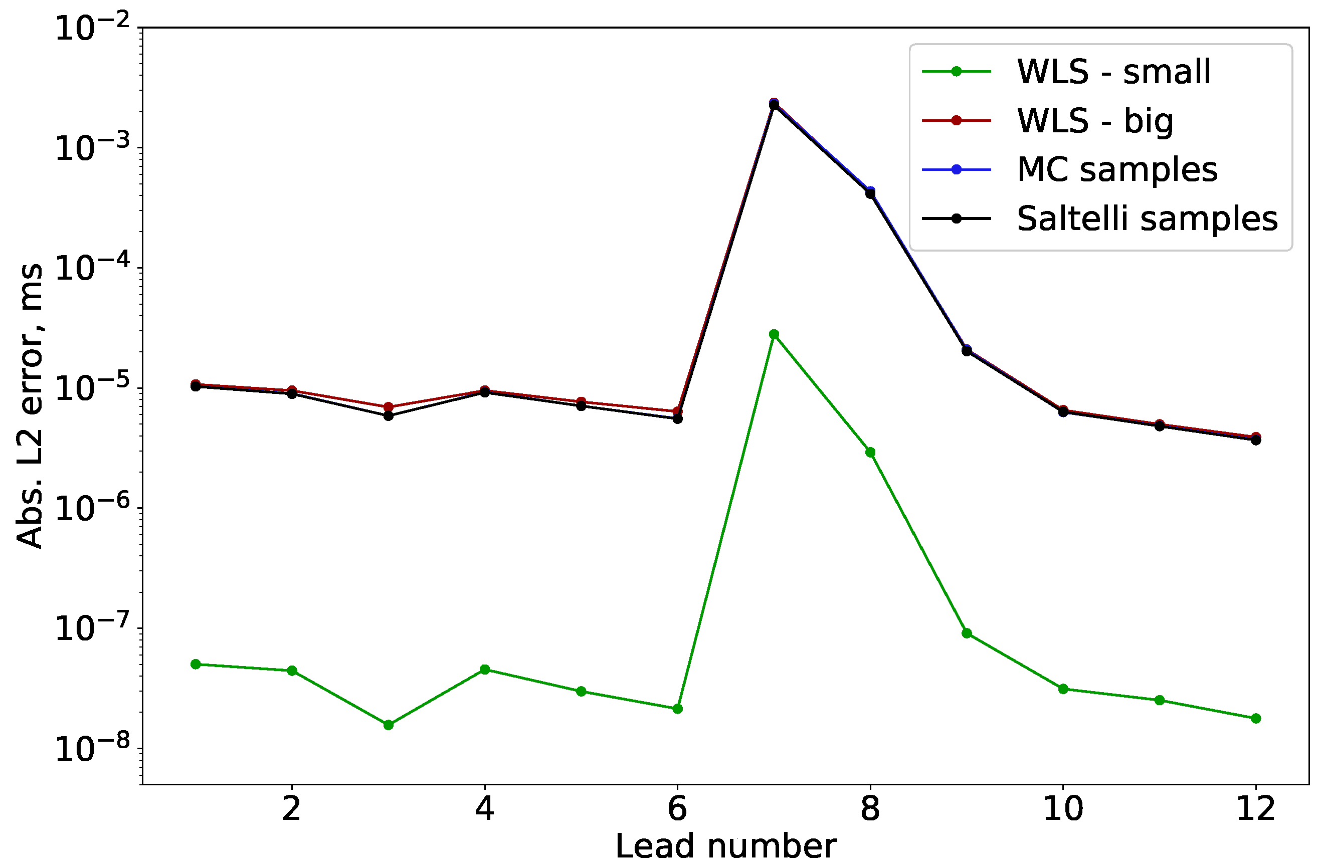
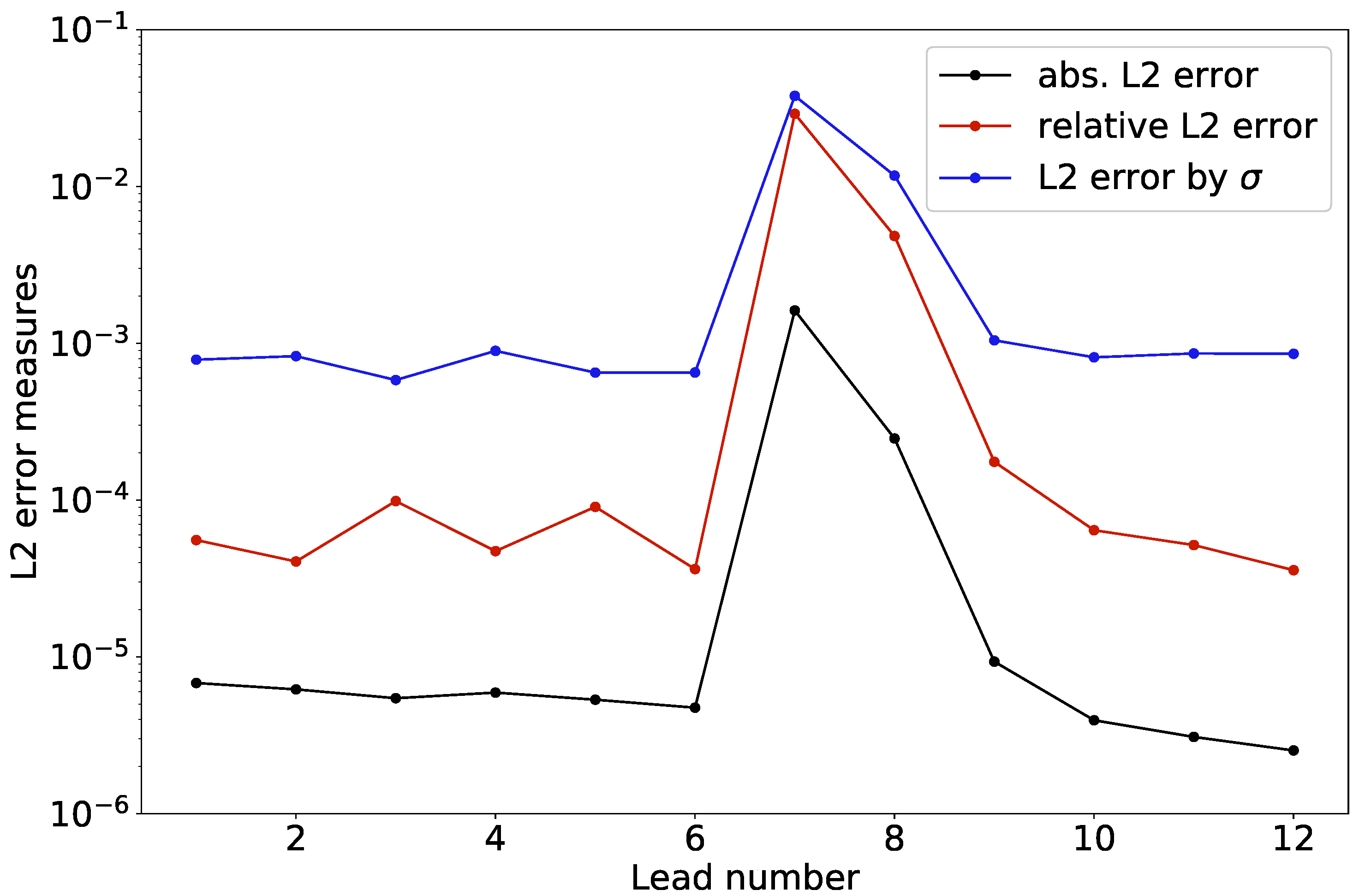
3.1.1. Error Estimation

The surrogate error can be estimated by splitting the dataset ( X ,   Y ) into two parts, a “training dataset” ( X t r a i n , Y t r a i n ) to construct the surrogate and a “test dataset” ( X t e s t , Y t e s t ) as ground truth data to compare the reconstructed ECG curves from the surrogate model to. The respective parameter tuples of the test data ( X t e s t ) are then used as an input for the constructed surrogate, yielding the reconstructed ECG signal { s P C } (or Y t e s t ). It is then possible to calculate the L 1 ( ϵ 1 ) and L 2 errors ( ϵ 2 ) of a reconstructed signal with respect to the corresponding ground truth signal s G T with the same tuple of input parameters.
ϵ 1 = 1 t s 0 t s | s G T ( t ) s P C ( t ) | d t
ϵ 2 = 1 t s 0 t s ( s G T ( t ) s P C ( t ) ) 2 d t ,
where t s is the signal length. ϵ 1 and ϵ 2 are then averaged over the whole test dataset X t e s t to yield representative spot samples with regard to the chosen input parameter interval, estimating the true value. Hence, to obtain a good estimate of the overall (mean) error of the surrogate model on the chosen interval, some measure of coverage has to be achieved by the size and distribution of the testing dataset, too. Here, we chose to take N = 500 test samples from the uniformly sampled parameter interval to average the L 1 and L 2 surrogate errors over, i.e., ϵ ¯ = 1 500 Σ i ϵ i . The standard deviation from this sample can additionally inform on the reliability of the error estimate. However, this estimate still exhibits some uncertainty due to the specific set of test data ( X t e s t ,   Y t e s t ) , therefore, we repeat the surrogate calculation typically ten times with different test and training data splits and the average over those 10 iterations informs Figure 3, Figure 4 and Figure 5.
For the assessment of the surrogate, we chose to consider the L 2 error because this formulation weights larger deviations between PC and ground truth signal stronger and reflects the least-squares minimization in the regression algorithm that determines the PCE coefficients. In Figure 3, the absolute L 2 errors for the 12 leads of the four datasets are shown on a logarithmic scale. Note that ϵ 2 for the dataset with small parameter variations (green) is significantly smaller and the three datasets with larger input parameter ranges exhibit nearly the same L 2 error, i.e., the difference with respect to different sampling schemes is very small.
Note also how the error varies between the different leads in a similar manner as the signal variance in Figure 2d. This is an indication that a large dataset output variance, rather than a larger signal strength leads to less accurate PCE surrogates. With that, we have two possible means to contextualize the obtained error measures: by normalizing the values either by signal strength or by signal variance, cf. Figure 4.

3.1.2. Normalization of the Surrogate Error

The absolute L 2 error as described above is already a good indicator to monitor the increase in accuracy of the surrogate model. However, it is quite difficult to obtain a sense of “small” or “big” approximation errors by just observing ϵ 2 without reference. A way to contextualize the L 2 error is to normalize it by dividing it by either the signal strength S as defined in Equation (9) or by the signal variance of the dataset σ as defined in Equation (8). In the first case, one obtains a relative error measure analogous to a signal to noise ratio. The relative L 2 error reads:
ϵ 2 , r = 1 N i 1 t s t [ s G T , i ( t ) s P C , i ( t ) ] 2 d t 1 t s t | s G T , i ( t ) | d t = 1 N i ϵ 2 , i s i
In this sense, an approximation error of ϵ 2 = 1 % means that of the complete ECG curve, the mean deviation between reconstructed and simulated data (ground truth) is 1 % of the signal itself. Hence, the normalization with signal strength alleviates the problem of different scales of output parameters. The relative L 2 error of the MC DS (DS 3), reconstructed in sixth order is given in Figure 4 in red.
In general, we observe that with a higher output variance it becomes harder to construct precise surrogate models, cf. Figure 2d. This higher spread in the output data can be caused by broader input parameter intervals (as exemplified by the comparison with the dataset with smaller input variance), or a stronger dependence of the output on input parameters (due to the position in parameter space or the choice of input parameters). In our case, lead V1 (number 7) exhibits significantly larger output variance, which also results in a larger surrogate error. Hence, one meaningful information of the surrogate convergence is to compare the approximation error ϵ ^ with an appropriately chosen variation measure of the dataset. By dividing the L 2 error by the standard deviation σ , the square root of the signal variance (cf. Equation (8)), one compares how much better the reconstructed curve is with respect to a randomly chosen one out of the dataset ( X ,   Y ) . For an illustration of the DS output variability, cf. Figure 2a,b. There, the mean signal of the Monte–Carlo sampled dataset is given in black together with the 1 σ interval in red, for the lead number 1 (I) with a relatively small signal variance and for the lead number 7 (V1) with the largest signal variance of all 12 leads.
For clarification of the units used in Figure 4, the absolute L 2 error is a measure of the squared signal differences (given in [ ( mV ) 2 ]), integrated over and divided by signal length [ ms ] [ ms 1 ] . By taking the square root, the units hence become [ mV ] . Analogously, the standard deviation σ of the output and the mean signal strength S have the same units. Hence, the two derived, relative error measures are unitless in Figure 4.

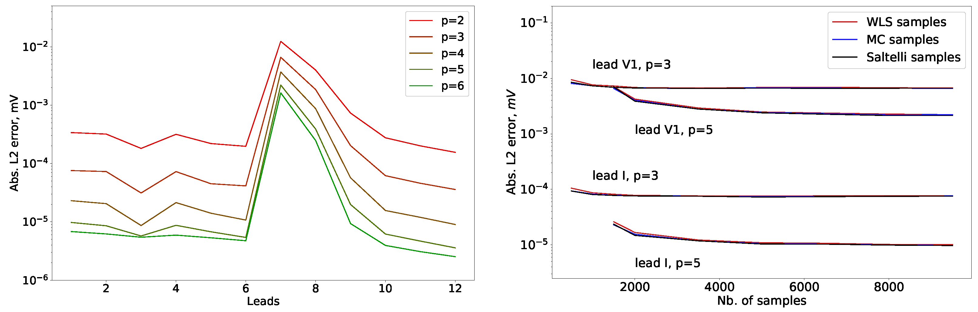
3.1.3. Surrogate Error Convergence

We are interested in two types of surrogate error convergence: The first is the increase in accuracy with respect to an increasing polynomial order p used to construct the surrogate. It is straight-forward that with a higher degree of polynomial order, the number of expansion terms of the surrogate increases and the truncation error introduced in Equation (4) becomes smaller. However, this stands against two types of restrictions—the computational constraints such as calculation times, RAM usage and data storage size limit the attainable maximal order for the surrogate. Additionally, the number of terms to be determined by the regression has to be significantly smaller than the number of samples used in order to minimize the numerical error. In the first case, i.e., if the computational resources are the limiting factor, one observes a monotonic decrease in the surrogate error up to the maximal polynomial order feasible. In the second case, the number of samples is not large enough to allow for a good regression of all expansion coefficients of the surrogate (in the maximal polynomial order available). Hence, the total surrogate error (the sum of truncation and numerical error) increases again for the higher polynomial orders and the optimal surrogate has to be chosen with a p < p m a x . Depending on the cost of a single model evaluation, one can add further samples to decrease the numerical error of the higher order surrogate models.
The second convergence of interest is the behavior of the surrogate error with respect to sample size, i.e., how the L 2 error for a given surrogate model decreases with sample size. Possible points of interest are the rate of the error decrease (with number of samples) and the typical error levels for few and for many samples. If the number of samples is high enough so that the error does not further decrease when more are added, the numerical error is minimized and only a surrogate with higher polynomial order could achieve better precision (only the truncation error remains). One also expects differences between sampling schemes, i.e., the manner in which the samples for the generation of the surrogate models are distributed over the input parameter interval.

3.1.4. Convergence with Polynomial Order

For the first systematic study of surrogate models on the sampled data we vary the polynomial order p of the PCE method up to the maximum order given by computation time and hardware requirements. For the 8D datasets under consideration, this is the case for p = 6 , assuming the same degree for each input parameter. As usual (cf. Section 2.2) this also means restricting the maximum of the sum of the exponents p ^ of each term to the same value, p ^ = p . Hence, by systematically increasing the polynomial order, we examine the total surrogate error with a constant sample size of N s = 9500 . From the total number of samples N t o t = 10 , 000 , we leave 500 samples aside for estimating the surrogate error and construct different surrogate models for each of the leads independently. In Figure 5 on the left, we present the absolute L 2 errors of the Monte–Carlo-sampled dataset (DS 3), for p = 2 up to p = 6 for the 12 leads.
Generally, the L 2 error decreases with the polynomial order as expected, i.e., leading to better surrogate models for more expansion terms. Similarly to Figure 4, the leads show different L 2 errors, with lead 7 (V1) and 8 (V2) exhibiting significantly higher values. Even for the highest polynomial order, the surrogate errors differ by approximately two orders of magnitude.
From the convergence with polynomial degree up to order p = 6 , we estimate that a further increase in polynomial order would not bring significantly better surrogate accuracy, but a hugely increased computational load that would require computations on a dedicated server. Another possibility is to select different orders of expansion for the different parameters after a first construction with an equal number of basis polynomials. There, by selecting higher orders for the more influential parameters one would in principle expect an increase in the surrogate accuracy. However, we obtained no significant benefits that way on this dataset. We conclude that the desired level of surrogate accuracy for p = 6 is already sufficient for most of the leads and no significant benefit is to be expected in the cases of leads V1 and V2. The PCE surrogates for the leads except V1 and V2 are already very good for a surrogate model with the aim of substituting the computationally expensive original model. However, the main aim of the surrogate here is laying a foundation for SA and UQ, which has much less strict demands on surrogate accuracy. It is sufficient that the surrogate model rather closely resembles the underlying data as this determines, e.g., the reliability of the PCE-based Sobol indices (cf. Equation (7)) and the obtained surrogate models clearly allow for that.

3.1.5. Convergence with Sample Size

The convergence with sample size informs about the numerical error in determining the coefficients via linear regression, cf. Section 2.3. The overall approximation error of a surrogate model decreases with increasing sample size N s . Hence, if the statistically estimated error saturates with more samples used, one can be reasonably sure that it is only possible to further decrease the error by increasing the chosen polynomial order, cf. Figure 5 (right side). There, we varied the N s from 500 for 3rd order and 1500 for the 5th order up to the total number of 9500 (reserving 500 for estimating the L 2 error). Shown are two representative leads: lead number 1 (I) with very low approximation error and lead number 7 (V1) with the maximal error of the 12 leads. Further, we present surrogate models with two different maximal polynomial orders, up to 3rd and up to 5th order, to highlight the differences in the convergence behavior of the absolute L 2 error estimates. Qualitatively, the four chosen cases behave very similar as for low sample size the error is larger and steadily decreases until a plateau is reached. This shows that the overall approximation error is influenced by the numerical error for small N s , which quickly vanishes and the truncation error from the finite polynomial order of the considered PCE remains.
It becomes clear from the comparison of all four cases that the surrogate models with higher polynomial order exhibit significantly lower errors, but need more samples. The minimal number of samples to yield a sensible estimate is given by the well-posedness of the info matrix of the regression algorithm, essentially stating that as much samples are needed as there are independent expansion coefficients to be determined. The ensuing convergence is rather flat, i.e., the numerical error typically plays only a minor role in the construction of surrogate models in the presented case. For up to approximately 2000 samples for the 3rd order PCE and 4000 samples for the 5th order, the numerical error of determining the expansion coefficients still decreases. Similarly, one can estimate that in 6th order (the highest polynomial order used due to computational restrictions), the numerical error is also sufficiently small with 9500 samples. This is confirmed by the still smaller error estimates when compared to the 5th order, cf. Figure 5 (left side). Another systematic observation is that the three different sampling schemes yield nearly identical values, i.e., there are no important differences in convergence behavior, e.g., the minimal error for the convergence to arrive at a high number of samples or the convergence rate with sample size up to that point. For the tested schemes of WLS-optimized sampling, Monte–Carlo sampling and Saltelli sampling, only a very slight advantage for more evenly distributed samples (Saltelli > MC > WLS) was observed.
After evaluating the convergence of the surrogate accuracy with the maximal polynomial order and with sample size, we find that in the used datasets the surrogate errors of the best PCE models are dominated by the truncation error and the associated numerical error of determining the PCE expansion terms can be neglected for the 10,000 samples used. This finding is difficult to generalize because the model complexity, the dependence on different parameters and the chosen interval widths can result in markedly different DSs even for the same model to be analyzed. However, the described systematic analysis of the surrogate accuracy creates a valuable basis of the nature of the underlying DS, which will be used in SA and UQ later on as well as serves as a blueprint for the analysis of future datasets.

3.2. Sensitivity Analysis

One of the major advantages of constructing a surrogate model via PCE is the easy availability of the Sobol indices for SA, calculated simply by rearranging the expansion coefficients. Further, the error estimate of a surrogate gives an upper bound for the error of the obtained SIs (cf. Equation (7)) allowing for the monitoring of the SA accuracy. Qualitatively, the convergence is similar to the one of the overall L 2 errors, cf. Figure 5. However, the upper bound of the SI uncertainty varies greatly along the signal and can be evaluated with this level of detail by considering the mean L 1 error of the PCE surrogates over the signal.
In the following section we will present the main SA results, additional tabulated data can be found in the appendix. The obtained results and the impact on the modeling process of the underlying atria model (cf. Section 2.1) will be discussed after that.

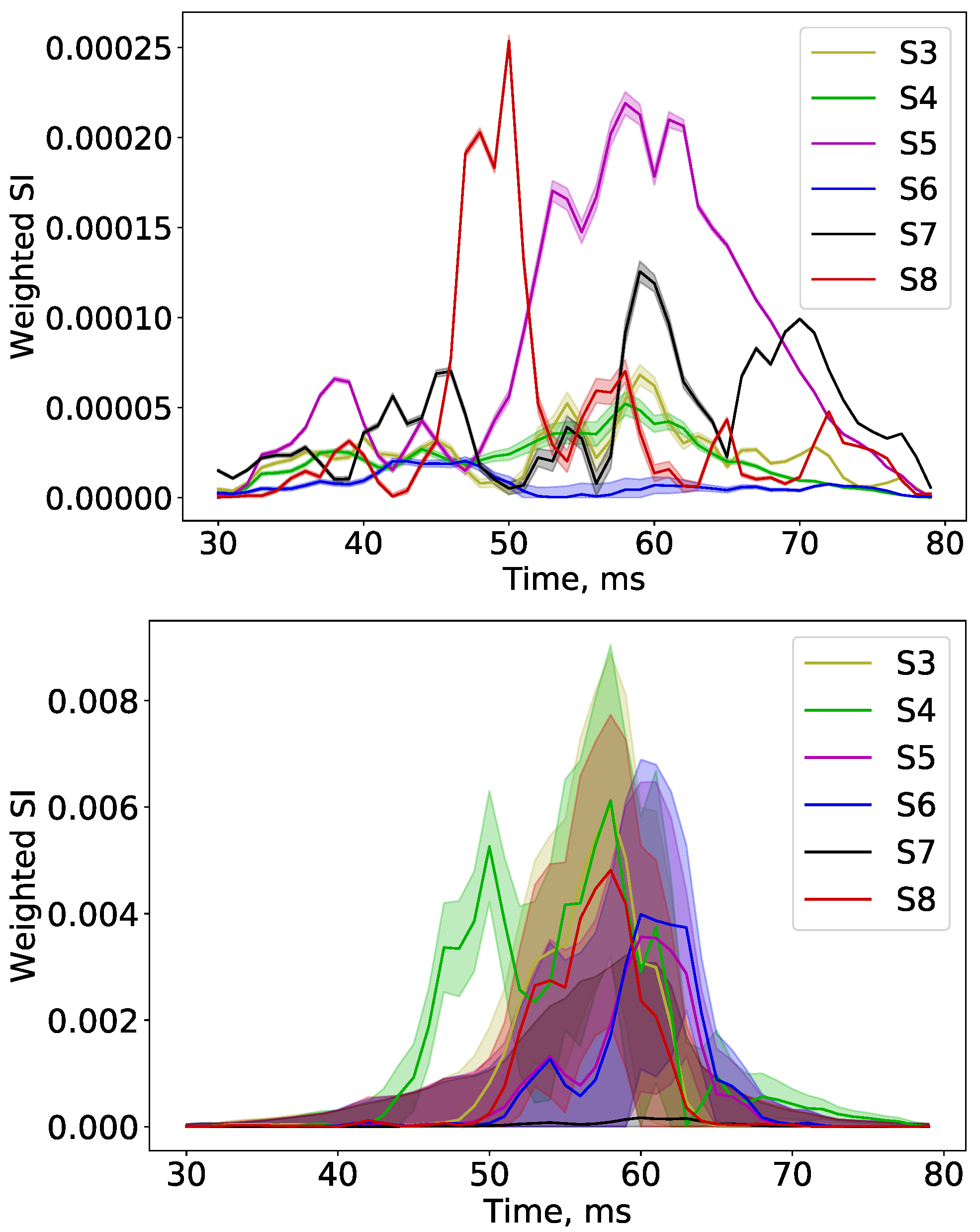
3.2.1. Sobol Indices along the Signal

One underlying simulation of the atria model results in a time-resolved signal, recorded in twelve different leads simultaneously with a time resolution of 1 ms and ≈150 ms length, leading to approximately 150 × 12 = 1800 data points. We then calculate the PCE for each lead separately and all output points of one lead are treated as independent output values for which the combined least squares are minimized by the regression algorithm of PyThia. Hence, from one surrogate model we obtain all individual SIs for each of the 150 signal points of one lead simultaneously. The SIs can vary between signal timepoints, yielding a time-resolved SA of the complete ECG signal.
Sobol indices are by definition adding up to one in each time point of the signal. However, in the context of assessing the importance of the input parameters on the ECG signal, it is more sensible to multiply them by the time-dependent signal variance σ 2 , cf. Figure 6 (upper and middle panel). Hence, the variance caused by the different input parameters (and parameter combinations for higher order SIs) can be traced over the whole signal and very detailed information, e.g., for fitting the model to a specific measured ECG is gained. This result for all 12 leads gives a first intuition for solving the inverse problem, i.e., determining the most likely set of parameters for a given ECG signal. The straight-forward intuition holds that the more influential input parameters are easier (i.e., more accurately) to reconstruct from signals in this inverse problem. However, this very detailed account of SA is in practice rather cumbersome and does not summarize the parameter importance very well, hence, we present a more concise measure in the following section.

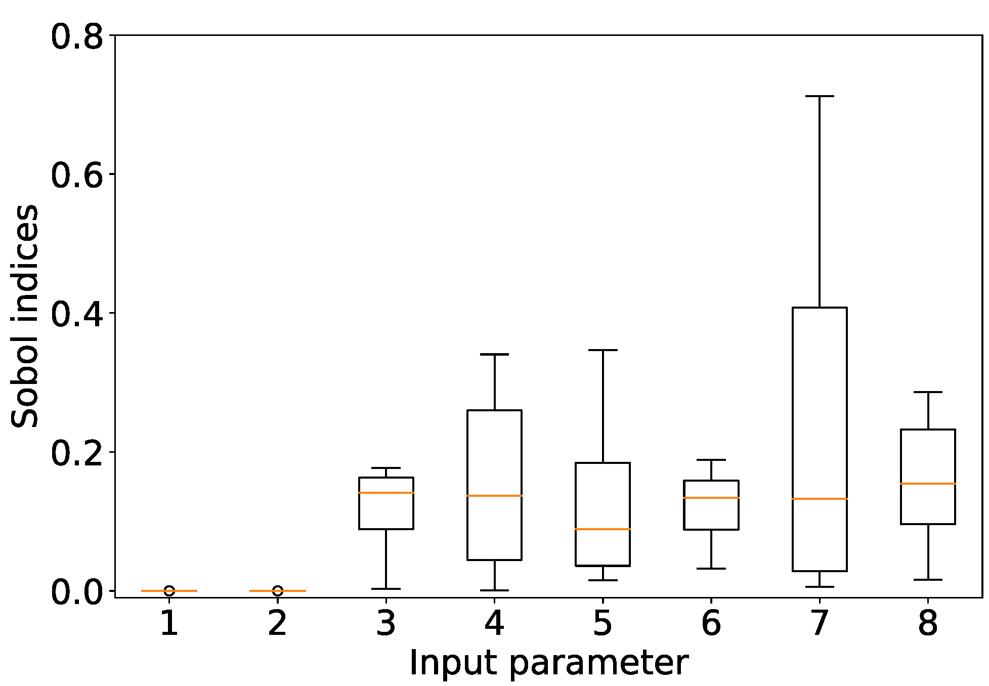
3.2.2. Time-Integrated Sobol Indices and Dataset Interpretation

By integrating the Sobol indices weighted by the time-dependent signal variance σ ( t ) over the signal length, one obtains a measure for the aggregate importance of that input parameter, or combinations of input parameters, on the ECG signal. For a convenient notation, we divide then by the integrated signal variance, again leading to SIs that add up to one:
S i n t = S ( t ) · σ 2 ( t ) d t σ 2 ( t ) d t
Additionally, we calculate the sum of all first order SIs as one measure of complexity of the dataset. Underlying this is the notion that the more of the data variance can be expressed in terms of single parameter variations, the simpler (or less complex) the uncertainty propagation from input parameters to output observables. Generally, this is the case for DSs with lower input and output variance—in analogy to a Taylor expansion it becomes clear that for an expansion of small variations around a given point in state space, a linear description by small, independent parameter variations is sufficient while for larger dataset variations, higher order terms become necessary for a precise description of the functional dependence. In our case, the results of the different leads of the presented DS confirms this trend empirically as lead V1 has the smallest score for the sum of first order SIs, cf. Table 2. Note also that, due to the cut-off of higher order terms in the definition of the PCE (cf. Section 2.3), higher order SIs are less precisely approximated. Hence, one can generally expect the three aspects to coincide: bigger contributions of high-order SIs, higher surrogate errors and more output variance in the dataset.
We can now summarize the SA of the presented synthetic ECG data by eight integrated SIs S i and the sum Σ S i for all twelve leads, i.e., 108 scalar values. As before, we constrain the presentation on the DS 3 because DS 2, 3 and 4 yielded very similar results and with DS 3 (10,000 Monte–Carlo samples) we do not have to assume any specific sampling strategy. Further, DS 1 was merely intended as a comparison for the increased surrogate quality with significantly lower input variability.
We see here that the Sobol indices of the first two parameters, the two conduction velocities, are very close to zero (in the order of 1 × 10 6 ). This means the two parameters have no discernible influence on the dataset, i.e., are not necessary to reconstruct data with a surrogate model and do not contribute appreciably to the signal variance. Second, all the other input parameters contribute to the signal variance in a heterogeneous way, i.e., for each lead the first order SIs differ significantly, although similarities between related leads can be found. Noteworthy are also the two highest single parameter contributions of over 70 % by the y-axis shift (parameter 7) in leads III and aVF. The sum of the first order SIs indicates that for most leads more than 90 % of the signal variance is covered by the single parameter variations. The exception form leads V1 and V2 with significantly lower proportions of the first order SI with 76 % and 84 % , respectively. This is in accordance with the higher surrogate error and signal variance we observe for those leads as the sum of the first order SI can be considered as a measure of dataset complexity. Hence, we hypothesize that with more output variance, generally also the higher-order parameter variations become important and with that the truncation error becomes more significant because the higher-order terms are cut by restricting the sum of all exponents to the maximum order of a single-parameter variation.
By averaging the values of the integrated SIs over all 12 leads, we can present a comprehensive picture of the dataset analysis, cf. Figure 6 (lower panel). Depicted there are the integrated SIs of all 12 leads as a box plot. The orange line indicates the median value, the box represents the upper and lower quartile and the whiskers indicate the data range. Again, we see that the conduction velocities (parameters 1 and 2) play no role in the description of the output variance of the DS. The three rotation angles (parameters 3, 4 and 5) as well as the three shifts (parameters 6, 7 and 8) contribute each about 10–15% to the output variance. The y-shift is appreciably more broadly distributed, indicating an especially variable importance of this parameter on the MC dataset.

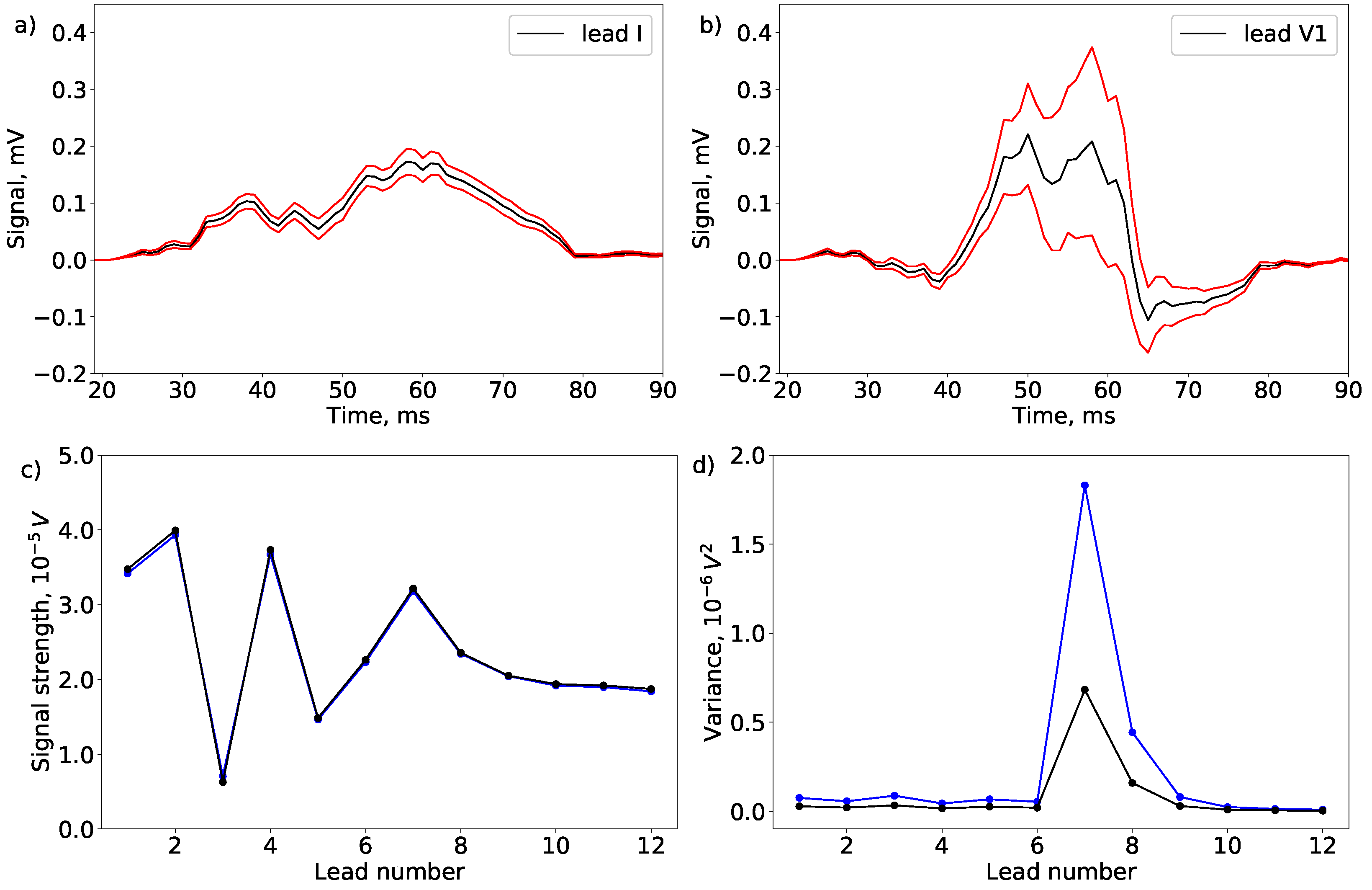
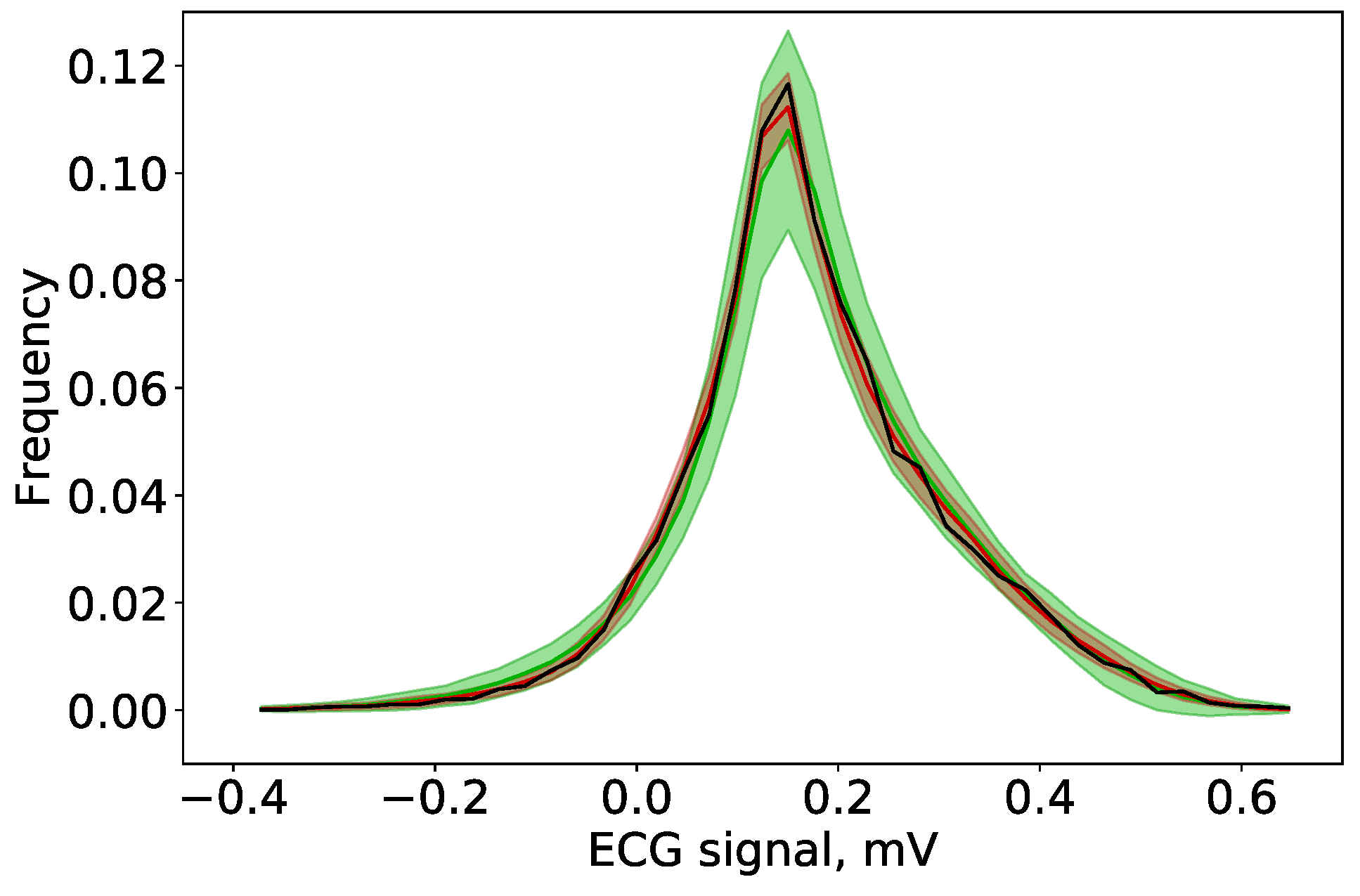
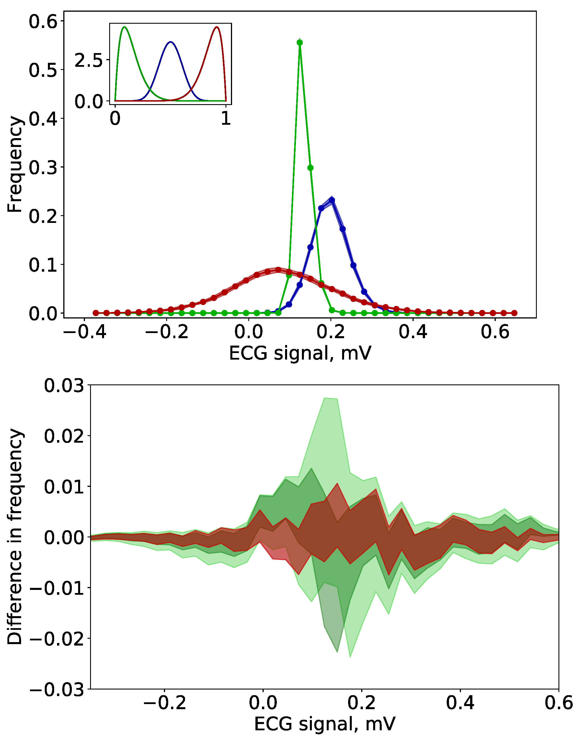
3.3. Uncertainty Quantification

With a calculated surrogate model it becomes also possible to address questions more concerned with the propagation and quantification of uncertainties. For a given distribution of the input parameters, each point in the ECG signal exhibits a specific distribution of values, too. The monitoring and description of the uncertainty propagation through a given model is referred to as uncertainty quantification (UQ). The depiction of mean signal and 1 σ band in Figure 2 can be considered as a basic example of UQ. With a surrogate model, however, we can re-sample easily and very quickly with different input parameter distributions and thereby study the propagation of uncertainty in a given model in great detail.
First, we have to validate the signal distributions we obtain via the surrogate model with the corresponding distributions of ground truth output values. For that, in Figure 7 in the top panel, the distributions of the Monte–Carlo sampled dataset are plotted in black for t = 55 ms (middle of the P-wave) in the signal of lead V1. For validation, we then sample the surrogate model in sixth polynomial order on the whole parameter interval it was constructed on (shown in red). We thereby use most of the possible 10,000 samples, merely reserving 100 random samples as a means to estimate the surrogate error. Note that instead of several days of computation time for 10,000 samples of the original model, we now only need a few seconds with a calculated PCE surrogate. To be able to ascertain the numerical stability of the sample distribution from different surrogates, we calculate 100 histograms from 10,000 samples each and over the 100 instances calculate the mean and standard deviation of the counts (the 2 σ band is depicted in light red). In order to compare the replication accuracy of statistical features, in contrast to single, complete signals, we also generated a very crude PCE surrogate of second polynomial order. In this case, only 45 and not ≈3000 terms have to be determined by the regression algorithm which means it is possible to use very few samples. Hence, we constructed 100 surrogate models with 100 samples, each chosen randomly from the complete set of 10,000 samples. Like for the sixth order surrogate, we depict the mean histogram with the 2 σ band in green and note that although the deviations between different histograms are significantly higher, the distribution of values is reproduced very well qualitatively.
To demonstrate UQ performed with a PCE surrogate, we sub-sample the sixth order surrogate model by employing an 8D beta-distribution by multiplying 8 univariate distributions: p ( x , α , β ) = x α 1 ( 1 x ) β 1 . The beta distribution is a sensible choice here because the support is finite, i.e., the same as the underlying (normalized) uniform distribution [ 0 , 1 ] N of the surrogate. Furthermore, for high values of the two defining parameters α = β , the beta distribution resembles the Gaussian distribution to a certain degree, a typical case for input parameter uncertainties in the frame of uncertainty quantification. Here, we consider three cases: α = β = 11 , resulting in a symmetric distribution, and also α = 11 , β = 2 and vise-versa for the asymmetric cases, respectively. Sampling from the defined input distribution results in a different distribution for the model output, i.e., the ECG signals, which are plotted in Figure 7 in blue. In principle, it thus becomes possible to address the propagation of any input uncertainty through the model to its output values as long as the support of the chosen input distribution is a subset of the support the surrogate model was constructed on.
To quantify the errors in reconstructing the signal distributions, we then considered the deviations with respect to the histogram of the Monte–Carlo sampled dataset, cf. Figure 7 in the bottom panel. More explicitly, we plotted the mean of the respective histograms over 100 instances, subtracted the ground-truth histogram and plotted the 2 σ band. Considered were three cases: first p = 6 constructed with N S = 9900 samples (as in Figure 7, lower panel, in red), second p = 2 with 100 samples (in light green) and third p = 2 with 9900 samples (in a darker shade of green), significantly reducing the deviations from the ground-truth data.

4. Discussion

We presented a method enabling sensitivity analysis (SA) and uncertainty quantification (UQ) of virtual 12-lead ECG data with the aid of a polynomial chaos expansion (PCE) surrogate model at the example of four P-wave datasets sampled in 8D parameter space. For that, we applied the established PCE method to time-dependent output data and used a non-intrusive implementation that determines the PCE coefficients based on linear regression on stochastic model evaluations from a defined input parameter distribution. The general scheme of the proposed SA/UQ methodology can be divided into three parts: We start with defining the specific DS we want to address by choosing the stochastic model parameters and their respective distributions, defining the input variability. In more elaborate models, where not all parameters can be addressed simultaneously, the choice of parameters itself is a process where groupings of parameter sets can be assembled, e.g., depending on meaning in the modeling context or by selecting only the most important ones (to be determined by a local analysis or a very crude, low-rank surrogate model). With that, a specific sampling scheme is chosen, i.e., the distribution and number of samples to be used on the input parameter space. The second step is to create the PCE surrogate on the sampled dataset. It is sensible to study its accuracy with respect to the chosen error measure and ascertain the optimal set of hyperparameters of the PCE, e.g., the maximal polynomial order for each parameter and whether more sampling is sensible, by a systematic analysis of the numerical and the truncation error. The obtained reliability of the surrogate then serves to inform the reliability of the last step, the performed SA and/or UQ. Directly from the expansion coefficients of the surrogate, we obtain the approximated Sobol indices for SA and based on the surrogate error also an upper bound on the precision of each SI, cf. Equation (7). With a surrogate model, it is much faster to sample additional model outputs, hence, the definition of arbitrary input parameter distributions (as long as their support is a subset of the initial parameter interval of the surrogate) and the subsequent evaluation of the resultant output distributions greatly enhances the capabilities to perform uncertainty quantification.
In the presented case, the choice of a sampling scheme yielded only tiny differences in the obtained surrogate accuracy and no qualitative differences in its convergence behavior, cf. Figure 5. However, the increase of the input parameter interval width (and subsequently the output variance) reduces the obtainable surrogate accuracy considerably, cf. Figure 3. Similarly, the differences in reconstruction accuracy between the separate leads are very large, which is related to the different output variances over the same input parameter interval. For the input dimension N i n = 8 , the maximal polynomial order to be calculated was p = 6 , which gives a surrogate with 3003 terms with a relative error (cf. Equation (12)) typically below 1 × 10 4 , which is a very good basis for SA and UQ. For the leads V1 and V2, however, the error estimates are significantly larger with 3 % and 0.5 % , respectively. The different accuracies obtained relate to the much larger output variance of those two leads with respect to the position and orientation changes of the atria relative to the surface torso model where the virtual electrodes are located. This larger signal variance in turn comes from the close proximity of cardiac sources to the electrodes that define the leads V1 and V2, i.e., V1 and V2 represent a very local measurement of potential differences directly above the heart that are much more sensitive to its geometric shifts and rotations. Other leads are obtained by measuring potential differences over a longer distance and further away from the physical position of the heart. As the main aim of the surrogate here is laying a foundation for SA and UQ—not the substitution of the numerical model—we judge the surrogate accuracy as sufficient for the purpose.
The calculated Sobol indices are very reliable for most leads, the significantly larger upper bound for the SI uncertainty in lead V1 is depicted in Figure 6 in the middle panel. However, the bounds represent the maximal possible error on the SIs and the trends clearly contained in the time-dependent sensitivity analysis are already quite informative for modeling purposes (like calibration and parameter optimization). The time-integrated SIs (cf. Figure 6, lower panel) show that of the 8 parameters addressed, the two conduction velocities (P1 and P2) do not contribute significantly to the signal variance. The three rotation angles and the three spatial shifts of the heart model inside the torso all exhibit similar importance, though their influence varies strongly between the different leads. The different parameter influences with respect to the whole set of 12 leads fulfills one prerequisite for potentially solving the inverse problem of electrocardiography, i.e., the determination of unknown model parameters from a given ECG signal. Regarding the use case of simulating ECG signals, these properties could be of great value in terms of generating large-scale synthetic datasets [13,74] with low computational effort, applicable, e.g., as input to machine learning models for arrhythmia classification [15] or as an emulator for simulation parameter inference.
With a PCE surrogate, the UQ of the underlying model is significantly enhanced, because of the very quick sampling by surrogate evaluations ( 5 × 10 5 samples in a about 90s on a conventional desktop machine). We exemplified this by first validating the statistical properties of the 6th order surrogate model with the MC dataset, cf. Figure 7 (upper panel). We then compared it with an extreme example for a cheap surrogate model and found that it reproduced the data distribution quite well. Hence, we note that for the investigation of statistical properties of a complex ground truth model, PCE provides a reliable and feasible systematic approach that works reasonably well even with low order and very sparse sampling. In order to demonstrate the strengths of a surrogate model further, we assumed different univariate input distributions for the parameters in form of different high-order Beta distributions, cf. Figure 7 in the middle panel. By sampling the surrogate from these distributions (which have to have a smaller or equal support than the created surrogate), one can quickly assess the different output distributions. By constructing and sampling from different scenarios of input variability, the propagation of parameter errors in computationally expensive model for cardiac dynamics becomes feasible. Supplementary points on the usage, limitations and further directions for PCE models in the field of cardiac engineering are elaborated on in Appendix B.

5. Conclusions

We have developed and implemented a framework for sensitivity analysis and uncertainty quantification in a biophysically and anatomically realistic three-dimensional numerical model for the electrical activity of the atria. Our emphasis was on assessing the influence of model parameters on the simulated P-wave which is the atrial contribution to the electrocardiogram (ECG). Since the standard metrological approach of using Monte–Carlo simulations are computationally prohibitive, we have used a nonintrusive polynomial chaos-based approximation of the forward model. The surrogate model increases the speed of computations for varying parameters by more than five orders of magnitude, from about 90s per simulation run of the full computational model to about 5 × 10 5 samples of the surrogate in the same time (both on an average desktop machine). It further allows for the quantification of parameter influences via Sobol indices and is in principle amenable to analytical examination. By estimating the surrogate approximation error it also provides bounds for the accuracy of the obtained sensitivities. Thus, it is capable of supporting and improving the creation of synthetic databases of ECGs from a virtual cohort mapping a representative sample of the human population based on physiologically and anatomically realistic three-dimensional models. With the study of the presented datasets of simulated P-wave signals, we applied the polynomial chaos expansion (PCE) to time-dependent data and exemplified the capabilities of surrogate-based sensitivity analysis and uncertainty quantification. The obtained sensitivities and their interpretation in the context of the underlying electrophysiology further helped to illuminate aspects of the numerical model and represent a basis for parameter optimization in high dimensions. We showed the convergence of the PCE for the specific example of atrial electrical activity as part of standard ECGs and calculated the PCE-based Sobol indices for sensitivity analysis of the datasets. The exceptional strength of the gPCE framework to capture parametric uncertainty was displayed by comparing UQ based on different surrogate models, revealing that the assessment of statistical properties is feasible with basic PCE surrogates build from few model evaluations. By specifically addressing the model variability with respect to the orientation and position of the virtual atria inside the torso, we took a step towards understanding how natural and healthy ECG variability is caused and by extension, how to discern it from pathological signal changes, evaluated for diagnostics. We aim to extend the work in the future to the signal of the ventricles which requires to investigate more model parameters, thus aiding a more complete understanding of realistic models of cardiac electrophysiology and in particular of ECG variability overall. Methods of sensitivity analysis and uncertainty quantification will be helpful in assessing virtual cohorts of models aimed at representing biological variability in a population, e.g., for simulating a representative set of human ECGs.

Author Contributions

Conceptualization, B.W., S.H. and M.B.; methodology, B.W., N.F. and S.H.; software, B.W. and N.F.; validation, B.W.; formal analysis, B.W.; data curation, B.W., C.N. and A.L.; writing—original draft preparation, B.W., C.N. and M.B.; writing—review and editing, B.W., C.N., S.H., N.F., A.L., O.D. and M.B.; visualization, B.W. and C.N.; supervision, A.L., M.B. and O.D.; project administration, M.B. and O.D.; funding acquisition, M.B. and O.D. All authors have read and agreed to the published version of the manuscript.

Funding

This research was done in the framework of the project “MedalCare (18HLT07)—Metrology of automated data analysis for cardiac arrhythmia management” has received funding from the EMPIR programme co-financed by the Participating States and from the European Union’s Horizon 2020 research and innovation programme.

Data Availability Statement

The data presented in this study are available on request from the corresponding author.

Conflicts of Interest

The authors declare no conflict of interest.

Abbreviations

The following abbreviations are used in this manuscript:
PCEPolynomial Chaos Expansion
SASensitivity Analysis
UQUncertainty Quantification
ECGElectrocardiogram
SISobol index
DSdataset
GTDground truth data

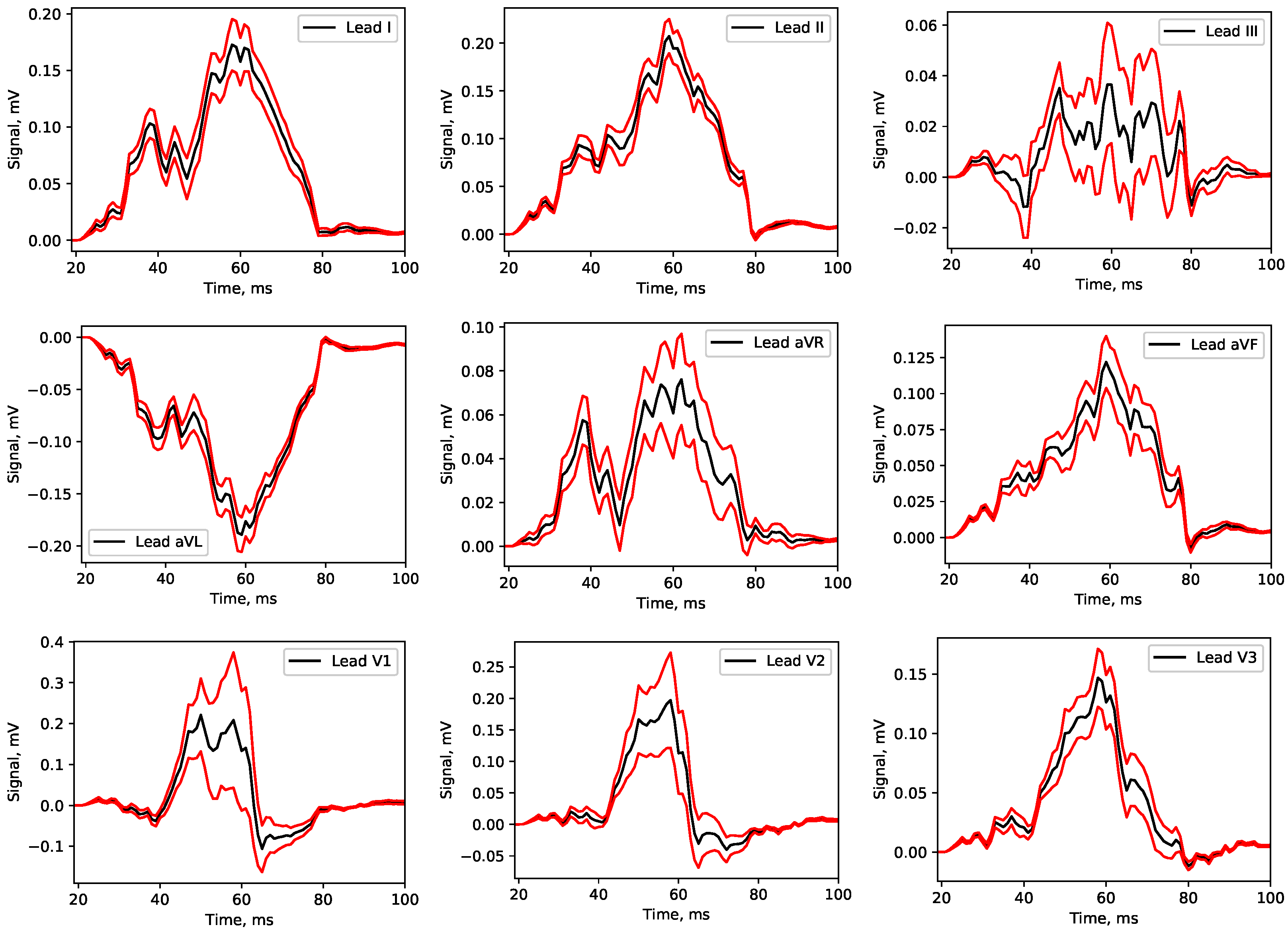
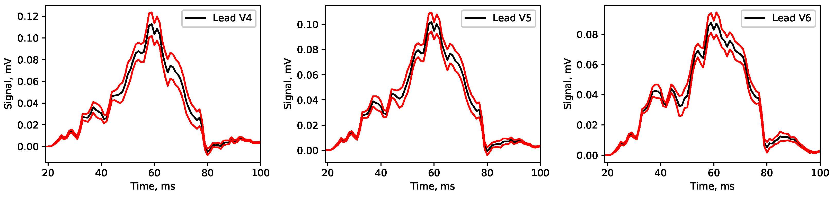
Appendix A. Mean Signals

Figure A1. The mean P-wave signal (black) of all leads in DS 3 and its range of ±one standard deviation (red).
Metrology 03 00001 g0a1aMetrology 03 00001 g0a1b

Appendix B. Usage, Limitations and Further Directions

The present study looked at the time dependent, 12-lead ECG curves of virtual atria. However, it is possible—and common in the community of computational cardiology—to look at certain features in the ECG, i.e., to derive a different output by introducing additional post-processing steps. It is equally feasible to create surrogate models for single features, typically intervals between or the amplitude of different peaks. For fitting a model to a specific patient, the closeness to some target output (e.g., via a fitness function) is also a valuable model output. Doing a sensitivity analysis on the feature space then enables modelers to address and communicate more specific questions about the model performance, e.g., it is easier to statistically match important ECG feature distributions, rather than matching a virtual cohorts of ECGs with measured ones [75] in a curve-by-curve matching scheme.
The numerical model for the generation of the P-wave datasets examined here exhibits >100 parameters that can be changed continuously, as well as meshes with ≈ 1 × 10 6 nodes where the system of PDEs is solved on (which can be parameterized via principle component analysis based on sample meshes). For the PCE surrogate, however, we can address only up to 12 parameters at a given time—depending on the necessary surrogate accuracy. Therefore, all datasets that can be evaluated represent a small, low-dimensional subspace of the complete parameter space. A possible expansion of the PCE scheme is the use of a low-rank representation (e.g., by employing the tensor train format) of the full coefficient tensor of the PCE model. Together with adaptive methods to chose only the most significant terms, the curse of dimensionality could be alleviated to some degree, enabling the treatment of more model parameters simultaneously.
However, a surrogate model itself can be useful for further analysis—especially if there are significant numerical or material costs of evaluating the original model. Single evaluations of a PCE surrogate are very fast, typically in the order of ms, and arbitrary input parameter distributions can be quickly assessed. One further option is to perform more involved data analysis such as machine learning on the numerically cheap surrogate and testing the reliability of the results with a smaller sample of the biophysically detailed model or experiment. A PCE surrogate is a linear combination of chosen basis polynomials, hence, it is typically easier to store, duplicate and transfer than the dataset itself and it is amenable to analytic treatment. Together with the much faster sampling capabilities, it becomes possible explore the high dimensional parameter space of involved numerical models much more directly. Conveniently for SA, the PCE-based Sobol coefficients and upper bonds on their error are easily accessible from the constructed PCE. Hence, one has to weigh the initial costs of the generation of a surrogate model with the benefits for SA and UQ, the flexibility and convenience of a surrogate, and the savings due to possible future model evaluations.

References

  1. Karma, A. Physics of cardiac arrhythmogenesis. Annu. Rev. Condens. Matter Phys. 2013, 4, 313–337. [Google Scholar] [CrossRef]
  2. Qu, Z.; Hu, G.; Garfinkel, A.; Weiss, J.N. Nonlinear and stochastic dynamics in the heart. Phys. Rep. 2014, 543, 61–162. [Google Scholar] [CrossRef] [Green Version]
  3. Alonso, S.; Bär, M.; Echebarria, B. Nonlinear physics of electrical wave propagation in the heart: A review. Rep. Prog. Phys. 2016, 79, 096601. [Google Scholar] [CrossRef] [PubMed] [Green Version]
  4. Rappel, W.J. The physics of heart rhythm disorders. Phys. Rep. 2022, 978, 1–45. [Google Scholar] [CrossRef]
  5. Loewe, A.; Wilhelms, M.; Fischer, F.; Scholz, E.P.; Dössel, O.; Seemann, G. Arrhythmic potency of human ether-a-go-go-related gene mutations L532P and N588K in a computational model of human atrial myocytes. Europace 2014, 16, 435–443. [Google Scholar] [CrossRef] [PubMed] [Green Version]
  6. Clayton, R.; Bernus, O.; Cherry, E.; Dierckx, H.; Fenton, F.H.; Mirabella, L.; Panfilov, A.V.; Sachse, F.B.; Seemann, G.; Zhang, H. Models of cardiac tissue electrophysiology: Progress, challenges and open questions. Prog. Biophys. Mol. Biol. 2011, 104, 22–48. [Google Scholar] [CrossRef] [PubMed]
  7. Bragard, J.R.; Camara, O.; Echebarria, B.; Giorda, L.G.; Pueyo, E.; Saiz, J.; Sebastián, R.; Soudah, E.; Vázquez, M. Cardiac computational modelling. Rev. Esp. Cardiol. (Engl. Ed.) 2021, 74, 65–71. [Google Scholar] [CrossRef]
  8. Dössel, O.; Luongo, G.; Nagel, C.; Loewe, A. Computer modeling of the heart for ECG interpretation—A review. Hearts 2021, 2, 350–368. [Google Scholar] [CrossRef]
  9. Corral-Acero, J.; Margara, F.; Marciniak, M.; Rodero, C.; Loncaric, F.; Feng, Y.; Gilbert, A.; Fernandes, J.F.; Bukhari, H.A.; Wajdan, A.; et al. The ‘Digital Twin’ to enable the vision of precision cardiology. Eur. Heart J. 2020, 41, 4556–4564. [Google Scholar] [CrossRef] [Green Version]
  10. Gillette, K.; Gsell, M.A.; Prassl, A.J.; Karabelas, E.; Reiter, U.; Reiter, G.; Grandits, T.; Payer, C.; Štern, D.; Urschler, M.; et al. A framework for the generation of digital twins of cardiac electrophysiology from clinical 12-leads ECGs. Med. Image Anal. 2021, 71, 102080. [Google Scholar] [CrossRef]
  11. Azzolin, L.; Eichenlaub, M.; Nagel, C.; Nairn, D.; Sánchez, J.; Unger, L.; Dössel, O.; Jadidi, A.; Loewe, A. AugmentA: Patient-specific Augmented Atrial model Generation Tool. medRxiv 2022. [Google Scholar] [CrossRef]
  12. Azzolin, L.; Eichenlaub, M.; Nagel, C.; Nairn, D.; Sanchez, J.; Unger, L.; Dössel, O.; Jadidi, A.; Loewe, A. Personalized ablation vs. conventional ablation strategies to terminate atrial fibrillation and prevent recurrence. EP Eur. 2022, 1–12. [Google Scholar] [CrossRef]
  13. Niederer, S.; Aboelkassem, Y.; Cantwell, C.D.; Corrado, C.; Coveney, S.; Cherry, E.M.; Delhaas, T.; Fenton, F.H.; Panfilov, A.; Pathmanathan, P.; et al. Creation and application of virtual patient cohorts of heart models. Philos. Trans. R. Soc. A 2020, 378, 20190558. [Google Scholar] [CrossRef]
  14. Nagel, C.; Luongo, G.; Azzolin, L.; Schuler, S.; Dössel, O.; Loewe, A. Non-Invasive and Quantitative Estimation of Left Atrial Fibrosis Based on P Waves of the 12-Lead ECG-A Large-Scale Computational Study Covering Anatomical Variability. J. Clin. Med. 2021, 10, 1797. [Google Scholar] [CrossRef]
  15. Wagner, P.; Strodthoff, N.; Bousseljot, R.D.; Kreiseler, D.; Lunze, F.I.; Samek, W.; Schaeffter, T. PTB-XL, a large publicly available electrocardiography dataset. Sci. Data 2020, 7, 154. [Google Scholar] [CrossRef]
  16. Zheng, J.; Fu, G.; Anderson, K.; Chu, H.; Rakovski, C. A 12-Lead ECG database to identify origins of idiopathic ventricular arrhythmia containing 334 patients. Sci. Data 2020, 7, 98. [Google Scholar] [CrossRef] [Green Version]
  17. Strodthoff, N.; Wagner, P.; Schaeffter, T.; Samek, W. Deep learning for ECG analysis: Benchmarks and insights from PTB-XL. IEEE J. Biomed. Health Inform. 2020, 25, 1519–1528. [Google Scholar] [CrossRef]
  18. Venton, J.; Harris, P.M.; Sundar, A.; Smith, N.A.; Aston, P.J. Robustness of convolutional neural networks to physiological electrocardiogram noise. Philos. Trans. R. Soc. A 2021, 379, 20200262. [Google Scholar] [CrossRef]
  19. Mehari, T.; Strodthoff, N. Self-supervised representation learning from 12-lead ECG data. Comput. Biol. Med. 2022, 141, 105114. [Google Scholar] [CrossRef]
  20. Mirams, G.; Pathmanathan, P.; Gray, R.; Challenor, P.; Clayton, R. White Paper: Uncertainty and variability in computational and mathematical models of cardiac physiology. J. Physiol. 2016, 594, 6833–6847. [Google Scholar] [CrossRef]
  21. Pathmanathan, P.; Gray, R. Ensuring reliability of safety-critical clinical applications of computational cardiac models. Front. Physiol. 2013, 4, 358. [Google Scholar] [CrossRef] [PubMed] [Green Version]
  22. Eck, V.G.; Donders, W.P.; Sturdy, J.; Feinberg, J.; Delhaas, T.; Hellevik, L.R.; Huberts, W. A guide to uncertainty quantification and sensitivity analysis for cardiovascular applications. Int. J. Numer. Methods Biomed. Eng. 2016, 32, e02755. [Google Scholar] [CrossRef] [PubMed]
  23. Quicken, S.; Donders, W.P.; van Disseldorp, E.M.; Gashi, K.; Mees, B.M.; van de Vosse, F.N.; Lopata, R.G.; Delhaas, T.; Huberts, W. Application of an adaptive polynomial chaos expansion on computationally expensive three-dimensional cardiovascular models for uncertainty quantification and sensitivity analysis. J. Biomech. Eng. 2016, 138, 121010. [Google Scholar] [CrossRef] [PubMed]
  24. Pathmanathan, P.; Cordeiro, J.M.; Gray, R.A. Comprehensive Uncertainty Quantification and Sensitivity Analysis for Cardiac Action Potential Models. Front. Physiol. 2019, 10, 721. [Google Scholar] [CrossRef] [PubMed] [Green Version]
  25. Montes, G.; Oliveira, J.; Alvarez-Lacalle, E.; Alonso, S.; Martins, B.; Weber, R. Combining polynomial chaos expansions and genetic algorithm for the coupling of electrophysiological models. In Lecture Notes in Computer Science: Bioinformatics and Biomedical Engineering 11538; Springer: Cham, Switzerland, 2019; pp. 116–129. [Google Scholar] [CrossRef]
  26. Costabal, F.S.; Matsuno, K.; Yao, J.; Perdikaris, P.; Kuhl, E. Machine learning in drug development: Characterizing the effect of 30 drugs on the QT interval using Gaussian process regression, sensitivity analysis, and uncertainty quantification. Comput. Methods Appl. Mech. Eng. 2019, 348, 313–333. [Google Scholar] [CrossRef]
  27. Hoffman, M.J.; Cherry, E.M. Sensitivity of a data-assimilation system for reconstructing three-dimensional cardiac electrical dynamics. Philos. Trans. R. Soc. A 2020, 378, 20190388. [Google Scholar] [CrossRef]
  28. Rupp, L.C.; Liu, Z.; Bergquist, J.A.; Rampersad, S.; White, D.; Tate, J.D.; Brooks, D.H.; Narayan, A.; MacLeod, R.S. Using uncertainSCI to quantify uncertainty in cardiac simulations. In Proceedings of the 2020 Computing in Cardiology, Rimini, Italy, 13–16 September 2020; pp. 1–4. [Google Scholar]
  29. Campos, J.; Sundnes, J.; Dos Santos, R.; Rocha, B. Uncertainty quantification and sensitivity analysis of left ventricular function during the full cardiac cycle. Philos. Trans. R. Soc. A 2020, 378, 20190381. [Google Scholar] [CrossRef]
  30. Lei, C.L.; Ghosh, S.; Whittaker, D.G.; Aboelkassem, Y.; Beattie, K.A.; Cantwell, C.D.; Delhaas, T.; Houston, C.; Novaes, G.M.; Panfilov, A.V.; et al. Considering discrepancy when calibrating a mechanistic electrophysiology model. Philos. Trans. R. Soc. A 2020, 378, 20190349. [Google Scholar] [CrossRef]
  31. Clayton, R.H.; Aboelkassem, Y.; Cantwell, C.D.; Corrado, C.; Delhaas, T.; Huberts, W.; Lei, C.L.; Ni, H.; Panfilov, A.V.; Roney, C.; et al. An audit of uncertainty in multi-scale cardiac electrophysiology models. Philos. Trans. R. Soc. A 2020, 378, 20190335. [Google Scholar] [CrossRef]
  32. Tate, J.D.; Good, W.W.; Zemzemi, N.; Boonstra, M.; Dam, P.v.; Brooks, D.H.; Narayan, A.; MacLeod, R.S. Uncertainty quantification of the effects of segmentation variability in ecgi. In Proceedings of the International Conference on Functional Imaging and Modeling of the Heart, Stanford, CA, USA, 21–25 June 2021; pp. 515–522. [Google Scholar]
  33. Narayan, A.; Liu, Z.; Bergquist, J.; Charlebois, C.; Rampersad, S.; Rupp, L.; Brooks, D.; White, D.; Tate, J.; MacLeod, R.S. Uncertainsci: Uncertainty Quantification for Computational Models in Biomedicine and Bioengineering. Comput. Biol. Med. 2022, 152, 106407. [Google Scholar] [CrossRef]
  34. Steinman, D.A.; Migliavacca, F. Special issue on verification, validation, and uncertainty quantification of cardiovascular models: Towards effective vvuq for translating cardiovascular modelling to clinical utility. Cardiovasc. Eng. Technol. 2018, 9, 539–543. [Google Scholar] [CrossRef] [Green Version]
  35. Mirams, G.R.; Niederer, S.A.; Clayton, R.H. The fickle heart: Uncertainty quantification in cardiac and cardiovascular modelling and simulation. Philos. Trans. R. Soc. A 2020, 378, 20200119. [Google Scholar] [CrossRef]
  36. Nagel, C.; Espinosa, C.B.; Gillette, K.; Gsell, M.A.; Sánchez, J.; Plank, G.; Dössel, O.; Loewe, A. Comparison of Propagation Models and Forward Calculation Methods on Cellular, Tissue and Organ Scale Atrial Electrophysiology. IEEE Trans. Biomed. Eng. 2022, 1–12. [Google Scholar] [CrossRef]
  37. Hoffman, B.F.; Rosen, M.R. Cellular mechanisms for cardiac arrhythmias. Circ. Res. 1981, 49, 1–15. [Google Scholar] [CrossRef] [Green Version]
  38. Keating, M.T.; Sanguinetti, M.C. Molecular and cellular mechanisms of cardiac arrhythmias. Cell 2001, 104, 569–580. [Google Scholar] [CrossRef] [Green Version]
  39. Tse, G. Mechanisms of cardiac arrhythmias. J. Arrhythmia 2016, 32, 75–81. [Google Scholar] [CrossRef] [Green Version]
  40. Luongo, G.; Vacanti, G.; Nitzke, V.; Nairn, D.; Nagel, C.; Kabiri, D.; Almeida, T.P.; Soriano, D.C.; Rivolta, M.W.; Ng, G.A.; et al. Hybrid machine learning to localize atrial flutter substrates using the surface 12-lead electrocardiogram. EP Eur. 2022, 24, 1186–1194. [Google Scholar] [CrossRef]
  41. BIPM; IFCC; ISO. IUPAP and OIML 2008, Supplement 1 to the ‘Guide to the Expression of Uncertainty in Measurement’—Propagation of Distributions Using a Monte Carlo Method JCGM 101: 2008; JCGM: Geneva, Switzerland, 2008. [Google Scholar]
  42. Rasmussen, K.; Kondrup, J.B.; Allard, A.; Demeyer, S.; Fischer, N.; Barton, E.; Partridge, D.; Wright, L.; Bär, M.; Fiebach, H.; et al. Novel Mathematical and Statistical Approaches to Uncertainty Evaluation: Best Practice Guide to Uncertainty Evaluation for Computationally Expensive Models; Euramet: Brunswick, Germany, 2015. [Google Scholar]
  43. Xiu, D. Numerical methods for stochastic computations. In Numerical Methods for Stochastic Computations; Princeton University Press: Princeton, NJ, USA, 2010. [Google Scholar]
  44. Smith, R.C. Uncertainty Quantification: Theory, Implementation, and Applications; Siam: Philadelphia, PA, USA, 2013; Volume 12. [Google Scholar]
  45. Ghanem, R.; Higdon, D.; Owhadi, H. Handbook of Uncertainty Quantification; Springer: Berlin/Heidelberg, Germany, 2017; Volume 6. [Google Scholar]
  46. Heidenreich, S.; Gross, H.; Bär, M. Bayesian approach to the statistical inverse problem of scatterometry: Comparison of three surrogate models. Int. J. Uncertain. Quantif. 2015, 5, 511–526. [Google Scholar] [CrossRef] [Green Version]
  47. Heidenreich, S.; Gross, H.; Bär, M. Bayesian approach to determine critical dimensions from scatterometric measurements. Metrologia 2018, 55, S201. [Google Scholar]
  48. Rynn, J.A.; Cotter, S.L.; Powell, C.E.; Wright, L. Surrogate accelerated Bayesian inversion for the determination of the thermal diffusivity of a material. Metrologia 2019, 56, 015018. [Google Scholar]
  49. Weissenbrunner, A.; Fiebach, A.; Schmelter, S.; Bär, M.; Thamsen, P.U.; Lederer, T. Simulation-based determination of systematic errors of flow meters due to uncertain inflow conditions. Flow Meas. Instrum. 2016, 52, 25–39. [Google Scholar] [CrossRef]
  50. Sudret, B. Global sensitivity analysis using polynomial chaos expansions. Reliab. Eng. Syst. Saf. 2008, 93, 964–979. [Google Scholar] [CrossRef]
  51. Loewe, A.; Krueger, M.W.; Platonov, P.G.; Holmqvist, F.; Dössel, O.; Seemann, G. Left and Right Atrial Contribution to the P-wave in Realistic Computational Models. In Lecture Notes in Computer Science; Springer: Cham, Switzerland, 2015; Volume 9126, pp. 439–447. [Google Scholar] [CrossRef]
  52. Courtemanche, M.; Ramirez, R.J.; Nattel, S. Ionic mechanisms underlying human atrial action potential properties: Insights from a mathematical model. Am. J. Physiol.-Heart Circ. Physiol. 1998, 275, H301–H321. [Google Scholar] [CrossRef] [PubMed]
  53. Odille, F.; Liu, S.; van Dam, P.; Felblinger, J.; Odille, F.; Liu, S.; van Dam, P.; Felblinger, J. Statistical Variations of Heart Orientation in Healthy Adults. In Proceedings of the 2017 Computing in Cardiology Conference (CinC), Rennes, France, 24–27 September 2017; Volume 44. [Google Scholar] [CrossRef]
  54. Stenroos, M.; Mäntynen, V.; Nenonen, J. A Matlab library for solving quasi-static volume conduction problems using the boundary element method. Comput. Methods Programs Biomed. 2007, 88, 256–263. [Google Scholar] [CrossRef] [PubMed]
  55. Schuler, S.; Tate, J.D.; Oostendorp, T.F.; MacLeod, R.S.; Dössel, O. Spatial Downsampling of Surface Sources in the Forward Problem of Electrocardiography. In Proceedings of the Functional Imaging and Modeling of the Heart; Coudière, Y., Ozenne, V., Vigmond, E., Zemzemi, N., Eds.; Lecture Notes in Computer Science; Springer International Publishing: Cham, Switzerland, 2019; Volume 11504, pp. 29–36. [Google Scholar] [CrossRef]
  56. Saltelli, A. Global sensitivity analysis: An introduction. In Proceedings of the 4th International Conference on Sensitivity Analysis of Model Output (SAMO 2004), Santa Fe, NM, USA, 8–11 March 2004. [Google Scholar]
  57. Ge, Q.; Menendez, M. Extending Morris method for qualitative global sensitivity analysis of models with dependent inputs. Reliab. Eng. Syst. Saf. 2017, 162, 28–39. [Google Scholar] [CrossRef]
  58. Sobol, I.M. Sensitivity analysis for non-linear mathematical models. Math. Model. Comput. Exp. 1993, 1, 407–414. [Google Scholar]
  59. Ye, M.; Hill, M. Chapter 10—Global Sensitivity Analysis for Uncertain Parameters, Models, and Scenarios. In Sensitivity Analysis in Earth Observation Modelling; Petropoulos, G.P., Srivastava, P.K., Eds.; Elsevier: Amsterdam, The Netherlands, 2017; pp. 177–210. [Google Scholar] [CrossRef]
  60. Morris, M.D. Factorial Sampling Plans for Preliminary Computational Experiments. Technometrics 1991, 33, 161–174. [Google Scholar] [CrossRef]
  61. Campolongo, F.; Cariboni, J.; Saltelli, A. An effective screening design for sensitivity analysis of large models. Environ. Model. Softw. 2007, 22, 1509–1518. [Google Scholar] [CrossRef]
  62. Sobol’, I. Global sensitivity indices for nonlinear mathematical models and their Monte Carlo estimates. Math. Comput. Simul. 2001, 55, 271–280. [Google Scholar] [CrossRef]
  63. Wiener, N. The homogeneous chaos. Am. J. Math. 1938, 60, 897–936. [Google Scholar] [CrossRef]
  64. Xiu, D.; Karniadakis, G.E. The Wiener–Askey Polynomial Chaos for Stochastic Differential Equations. SIAM J. Sci. Comput. 2002, 24, 619–644. [Google Scholar] [CrossRef]
  65. Ernst, O.G.; Mugler, A.; Starkloff, H.J.; Ullmann, E. On the convergence of generalized polynomial chaos expansions. ESAIM Math. Model. Numer. Anal. 2012, 46, 317–339. [Google Scholar] [CrossRef] [Green Version]
  66. Kaintura, A.; Dhaene, T.; Spina, D. Review of Polynomial Chaos-Based Methods for Uncertainty Quantification in Modern Integrated Circuits. Electronics 2018, 7, 30. [Google Scholar] [CrossRef] [Green Version]
  67. Farchmin, N.; Hammerschmidt, M.; Schneider, P.I.; Wurm, M.; Bodermann, B.; Bär, M.; Heidenreich, S. Efficient Bayesian inversion for shape reconstruction of lithography masks. J. Micro/Nanolith. MEMS MOEMS 2020, 19, 024001. [Google Scholar] [CrossRef]
  68. Saltelli, A. Making Best Use of Model Evaluations to Compute Sensitivity Indices. Comput. Phys. Commun. 2002, 145, 280–297. [Google Scholar] [CrossRef]
  69. Oakley, J.E.; O’Hagan, A. Probabilistic sensitivity analysis of complex models: A Bayesian approach. J. R. Stat. Soc. Ser. B (Stat. Methodol.) 2004, 66, 751–769. [Google Scholar] [CrossRef] [Green Version]
  70. Farchmin, N. Adaptive and Non-Intrusive Uncertainty Quantication for High-Dimensional Parametric PDEs. Ph.D. Thesis, TU Berlin, Berlin, Germany, 2022. [Google Scholar]
  71. Farchmin, N. PyThia Uncertainty Quantification Toolbox. Vers.: 2.0. 2021. Available online: https://gitlab1.ptb.de/pythia/pythia/ (accessed on 15 September 2022).
  72. Oseledets, I.V. Tensor-train decomposition. SIAM J. Sci. Comput. 2011, 33, 2295–2317. [Google Scholar] [CrossRef]
  73. Homma, T.; Saltelli, A. Importance measures in global sensitivity analysis of nonlinear models. Reliab. Eng. Syst. Saf. 1996, 52, 1–17. [Google Scholar] [CrossRef]
  74. Gillette, K.; Gsell, M.A.; Nagel, C.; Bender, J.; Winkler, B.; Williams, S.E.; Bär, M.; Schäffter, T.; Dössel, O.; Plank, G.; et al. MedalCare-XL: 16,900 healthy and pathological 12 lead ECGs obtained through electrophysiological simulations. arXiv 2022, arXiv:2211.15997. [Google Scholar]
  75. Nagel, C.; Pilia, N.; Loewe, A.; Dössel, O. Quantification of Interpatient 12-lead ECG Variabilities within a Healthy Cohort. Curr. Dir. Biomed. Eng. 2020, 6, 493–496. [Google Scholar] [CrossRef]
Figure 1. Overview of the atrial model used for the simulations, the top and bottom panels show the anterior and posterior view, respectively. The reference position of the atria within the torso as well as the electrode positions are visualized on the left side. On the right side, the atrial model is depicted with the tissue structures highlighted to which different conduction velocities were assigned.
Metrology 03 00001 g001
Figure 2. Characterization of the datasets. (a) The mean P-wave signal (black) of lead I and the range of ±one standard deviation (red) calculated over all 10,000 Monte–Carlo (MC) samples as an example of a lead with small overall signal variance. (b) The corresponding mean and 1 σ range for lead V1 with the highest overall variance. For a depiction of the corresponding signals for all leads, cf. appendix. (c) Left: The mean signal strength S for the 12 different leads, cf. Equation (9). Depicted are the Monte–Carlo sampled dataset with high input variability in blue and the dataset with small input variability in black, showing only minor differences. (d) Signal variance σ 2 of the 12 leads, cf. Equation (8). Depicted are the dataset with low input variability (DS 1 in black) and the MC-sampled dataset with high input variability (DS 3 in blue).
Metrology 03 00001 g002
Figure 3. Absolute L2 error estimates (cf. Equation (11)) for the PCE surrogates of the four different datasets with polynomial order p = 6 . Note that the differences between the three different sampling schemes, optimized for weighted least-squares (WLS, red), a standard Monte–Carlo sampling (MC, blue) and the Saltelli sampling scheme (black) yield very similar values of the approximation accuracy. The surrogate with smaller input parameter variability (halved interval width in each of the 8 input dimensions around the same mean value, shown in green) gives significantly smaller approximation errors. When further comparing it with the inter-lead variation in Figure 2, it becomes clear that the smaller signal variance, rather than a difference in (mean) signal strength, determines approximation accuracy.
Metrology 03 00001 g003
Figure 4. Error measures for the PCE surrogate model. Depicted are the absolute L 2 error ( ϵ 2 , black, in mV), the relative L 2 error ϵ 2 , r (red, cf. Equation (12)) and the L 2 error divided by the standard deviation of the output of the whole dataset (blue, cf. Equation (8)). The PCE surrogates were created in sixth order on the Monte–Carlo sampled dataset (9500 samples for construction and 500 for error estimation). The inter-lead variation is similar to the variance of the sampled dataset, cf. Figure 2, with significantly higher approximation errors for the leads V1 and V2 (numbers 7 and 8).
Metrology 03 00001 g004
Figure 5. Error convergence for PCE surrogate models. (Left): Convergence of the absolute L 2 error with polynomial order p for the Monte–Carlo sampled dataset, shown for all 12 leads. (Right): The model error convergence with sample size for all DSs with high input variability. Shown are four different cases: Lead V1 with generally higher approximation errors, compared to lead I for two different orders of approximation, p = 3 and p = 5 . The saturation of the errors with sample size indicate that enough samples were used for the chosen polynomial order. Note that the higher polynomial order leads to smaller approximation errors but more samples are needed for the error to saturate at its minimum value. We observe only minor differences with respect to the sampling scheme used with very slight systematic advantages of the Saltelli samples and slightly higher errors for the WLS-optimized sampling, when compared to the Monte–Carlo sampling scheme.
Metrology 03 00001 g005
Figure 6. The first order Sobol indices S ( t ) i , weighted by signal variance σ 2 for lead I (Top) and lead V1 (Middle) for the Monte–Carlo sampled dataset. Note how parameter importance of P3–P8 varies with time and also between leads. All Sobol indices are multiplied by the signal variance to show the relevant influence on the EGC signal. The upper bound for uncertainty in determining Sobol indices (colored band around the mean values) is significantly larger in lead V1 when compared to lead I due to the higher approximation error, cf. Equation (7). (Bottom): The box plot of all first order, integrated Sobol indices (cf. Equation (13)) calculated for all leads. S1 and S2 are close to zero. For the other input parameters, we calculate comparable sensitivity measures overall (between 10 and 20 % ), although the inter-lead variations differ.
Metrology 03 00001 g006aMetrology 03 00001 g006b
Figure 7. Comparison of distributions of ECG values at a fixed time point ( t = 55 ms) in the signal of lead V1 (cf. Figure 2 in the upper right panel). (Top): The statistical properties of the Monte–Carlo sampled ground truth dataset (black, 10,000 samples) agree very well with the spectrum of values of the PCE approximations. A good PCE model ( p = 6 and N S = 9900 , depicted in red) and contrasting, a very basic one ( p = 2 and N S = 100 , in green) agree very well in the depicted 2 σ bands, respectively. (Middle): The surrogate model allows for a quick re-sampling for a more versatile UQ. As an example, all input parameters were sampled from either of the three Beta distributions p β shown in the inlay (the color coding matches the obtained output distributions), cf. text for more details. (Bottom): The deviations from the histogram of the ground truth data (GTD, cf. black line in the top panel) for three different PCE surrogate models. The mean and 2 σ band are depicted for p = 2 and N S = 100 in light green, p = 2 and N S = 9900 in dark green and p = 6 and N S = 9900 in red. With an increase in polynomial order and the number of samples underlying the determination of PCE coefficients, we generally see a better approximation of GTD, but the statistical properties can be reconstructed remarkably good even for very basic PCE surrogates.
Metrology 03 00001 g007aMetrology 03 00001 g007b
Table 1. Model parameters and intervals to sample from for generating the datasets with small and large parameter variations.
Model ParameterSmall VariationLarge Variation
CV (bulk tissue) [ 0.531 m s , 0.650 m s ] [ 0.473 m s , 0.709 m s ]
CV (interatrial connections) [ 0.580 m s , 0.710 m s ] [ 0.516 m s , 0.774 m s ]
translation X[−10 mm, 10 mm][−20 mm, 20 mm]
translation Y[−10 mm, 10 mm][−20 mm, 20 mm]
translation Z[−10 mm, 10 mm][−20 mm, 20 mm]
angle X[ 7.5 ° , 7.5 ° ][ 15 , 15 ]
angle Y[ 7.5 ° , 7.5 ° ][ 15 , 15 ]
angle Z[ 7 . 5 , 7.5 ° ][ 15 , 15 ]
Table 2. First order, PCE-based Sobol indices. The time-dependent indices were integrated over the complete signal length and are depicted here for all 12 leads and input parameter addressed (P1 and P2 (conduction velocities), P3–P5 (rotation angles) and P6–P8 (shifts of the atria within the torso)).
IIIIIIaVLaVRaVFV1V2V3V4V5V6
S 1 0.0000.0000.0000.0000.0000.0000.0000.0000.0000.0000.0000.000
S 2 0.0000.0000.0000.0000.0000.0000.0000.0000.0000.0000.0000.000
S 3 0.1060.1360.0030.1770.0320.0380.1620.1760.1650.1190.1570.146
S 4 0.0920.1190.0010.1550.0270.0320.2500.2830.3210.3400.2520.049
S 5 0.3460.0390.1670.2360.2940.0370.1030.1390.0750.0240.0150.034
S 6 0.0320.1540.0900.0820.0450.1440.1100.1240.1850.1890.1720.154
S 7 0.2020.3780.7100.0620.4970.7130.0060.0160.0200.0310.0640.318
S 8 0.1760.1380.0160.2310.0790.0240.1270.1020.1710.2490.2860.236
Σ S i 0.9540.9630.9880.9430.9740.9860.7580.8400.9370.9520.9460.938
Disclaimer/Publisher’s Note: The statements, opinions and data contained in all publications are solely those of the individual author(s) and contributor(s) and not of MDPI and/or the editor(s). MDPI and/or the editor(s) disclaim responsibility for any injury to people or property resulting from any ideas, methods, instructions or products referred to in the content.

