
Uncertainty-Based Autonomous Path Planning for Laser Line Scanners


Abstract
:1. Introduction
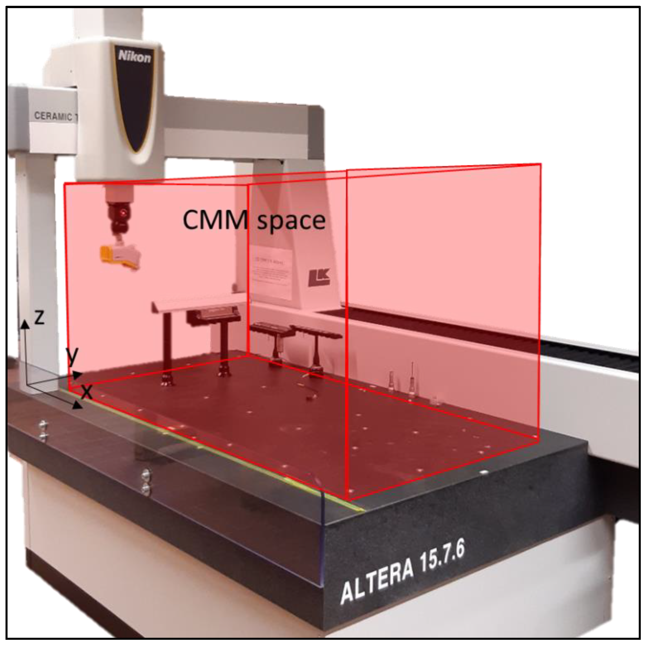
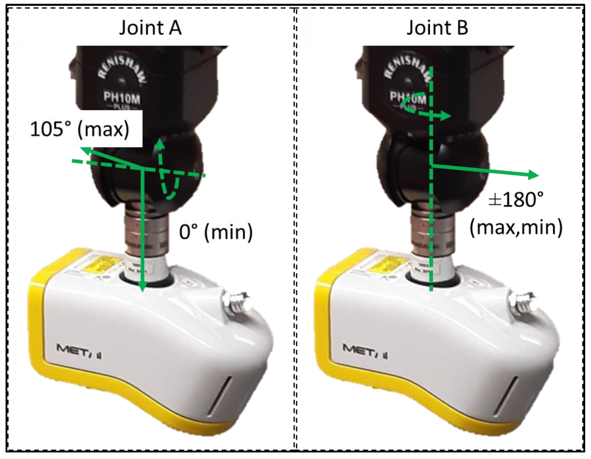
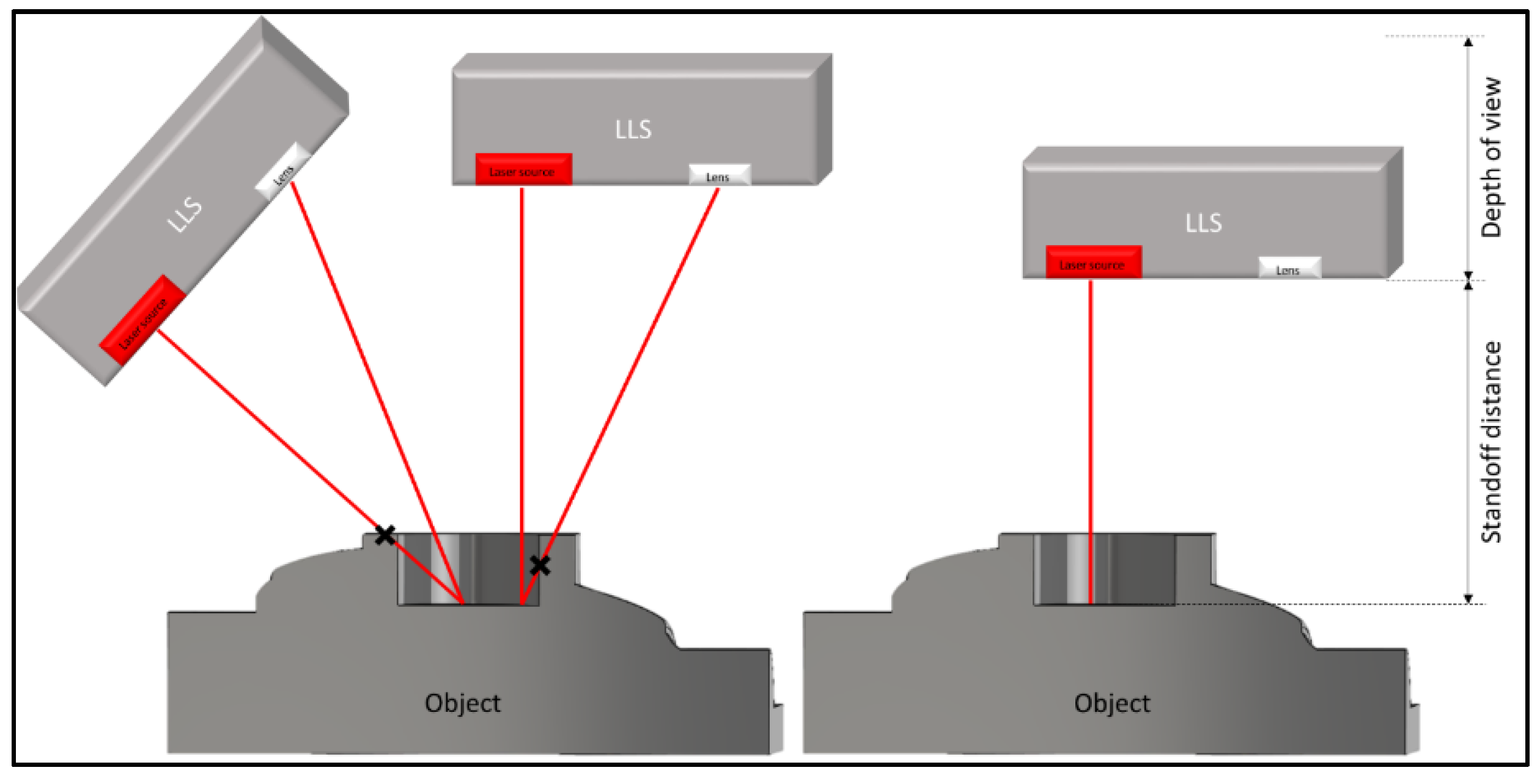
2. Optical Measurement System
3. Path Planning Algorithms: State-of-the-Art
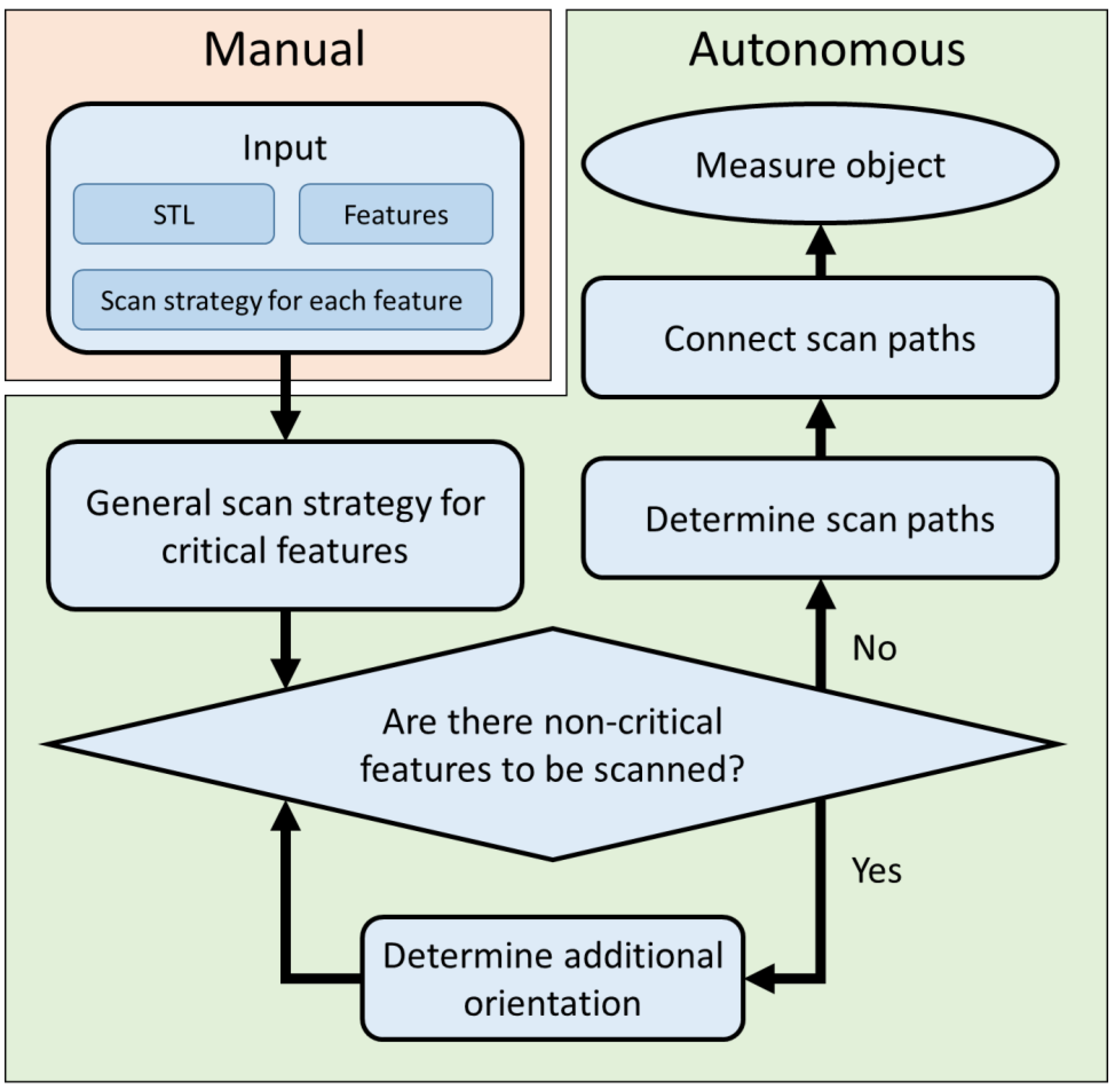
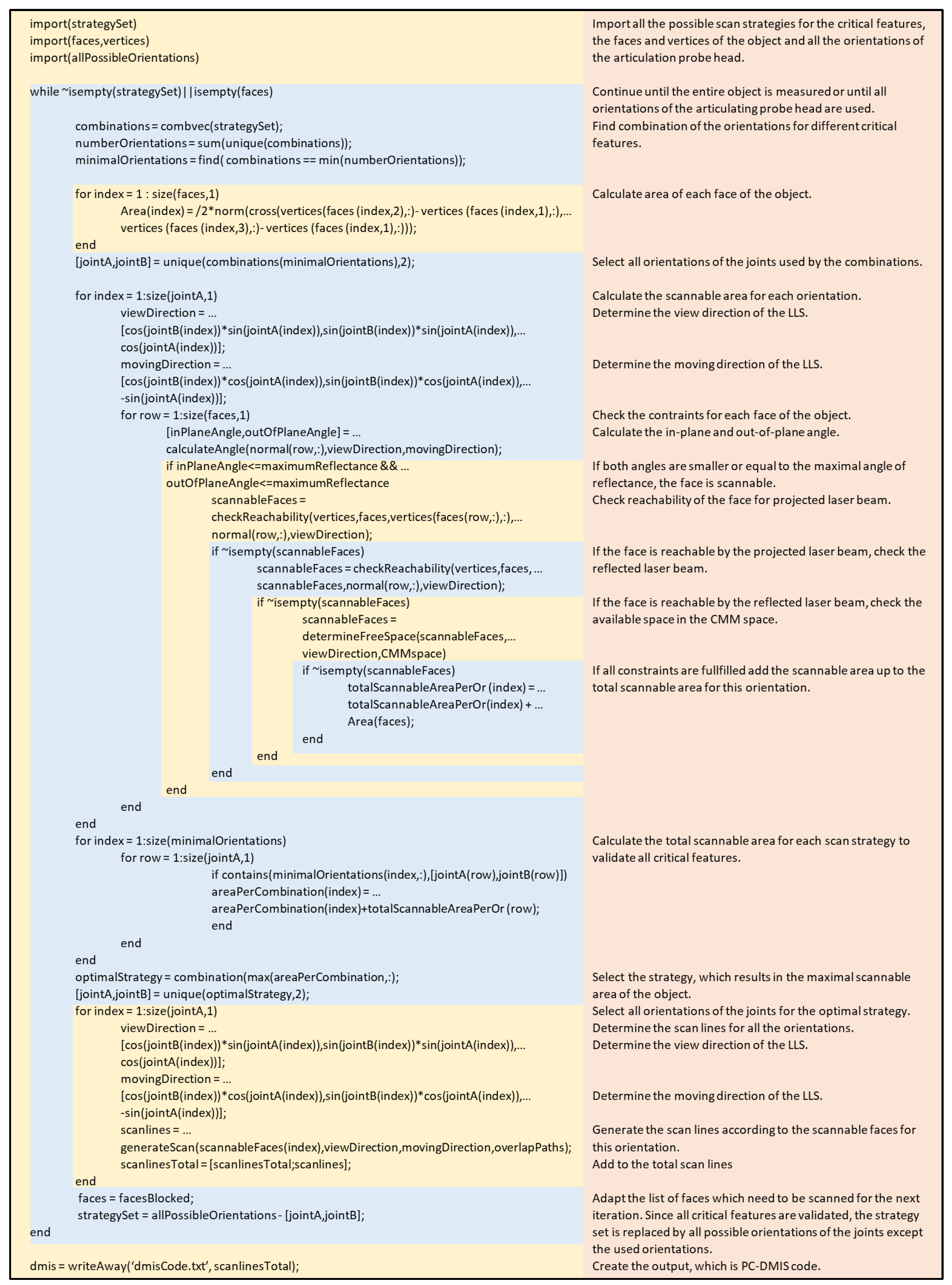
4. Algorithm
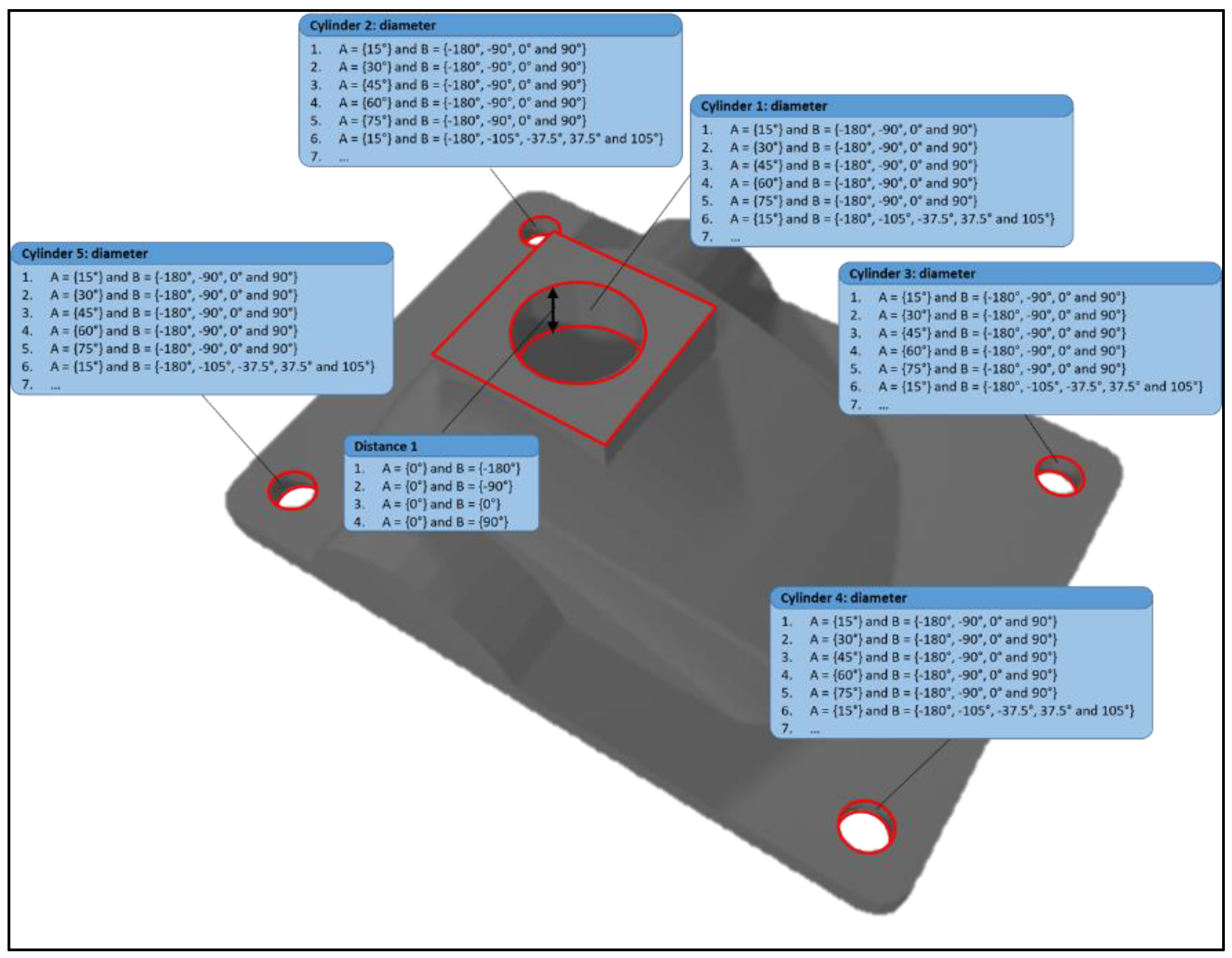
4.1. Step 1: Input
4.2. Step 2: General Scan Strategy for Critical Features
4.2.1. Step 2a: Minimum of Different Orientations
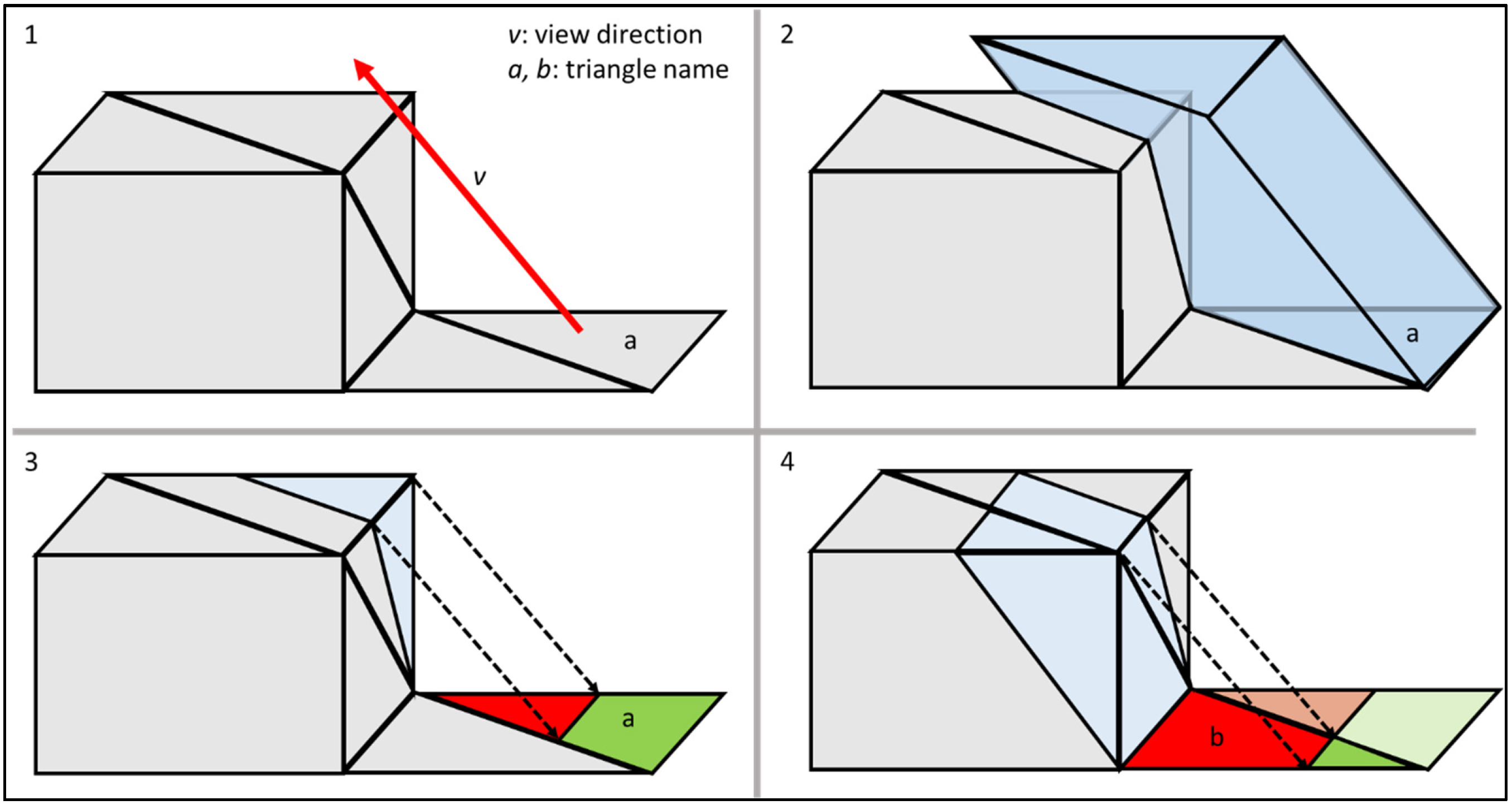
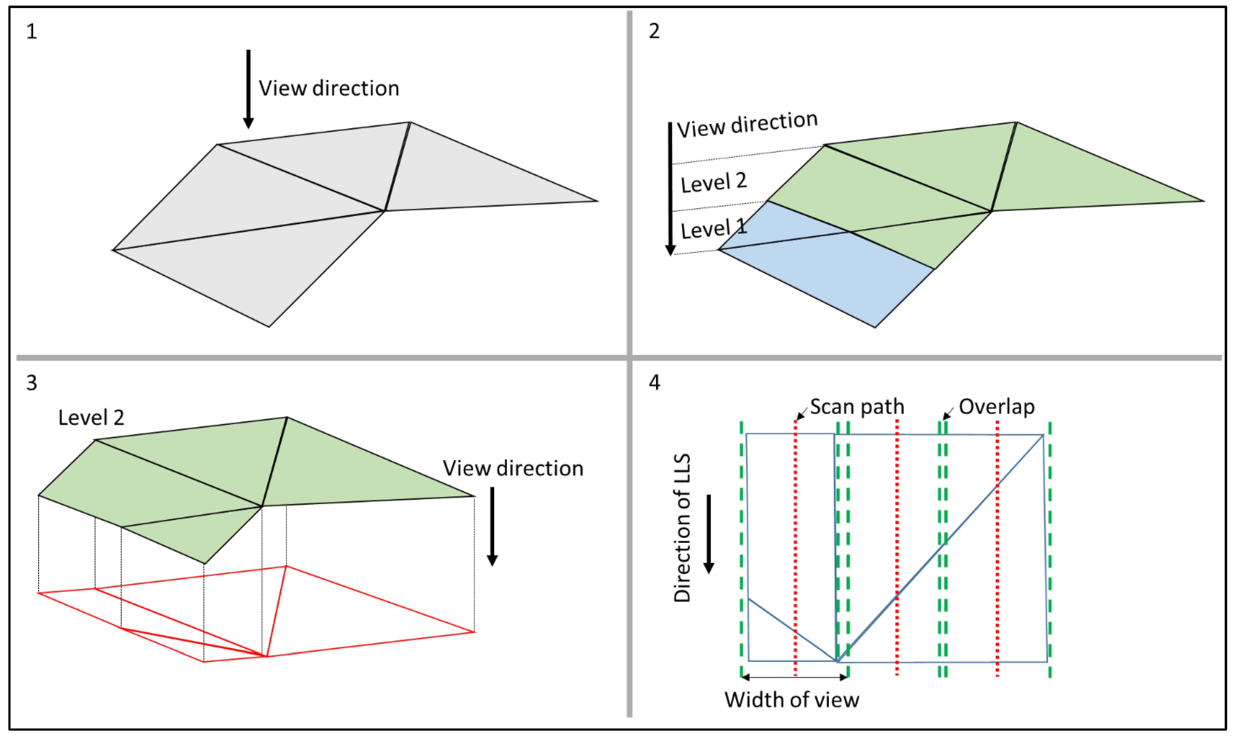
4.2.2. Step 2b: Calculate the Coverable Surface Per Orientation
4.2.3. Step 2c: Select Combination with Largest Scanned Surface
4.3. Step 3: Determine Additional Orientation
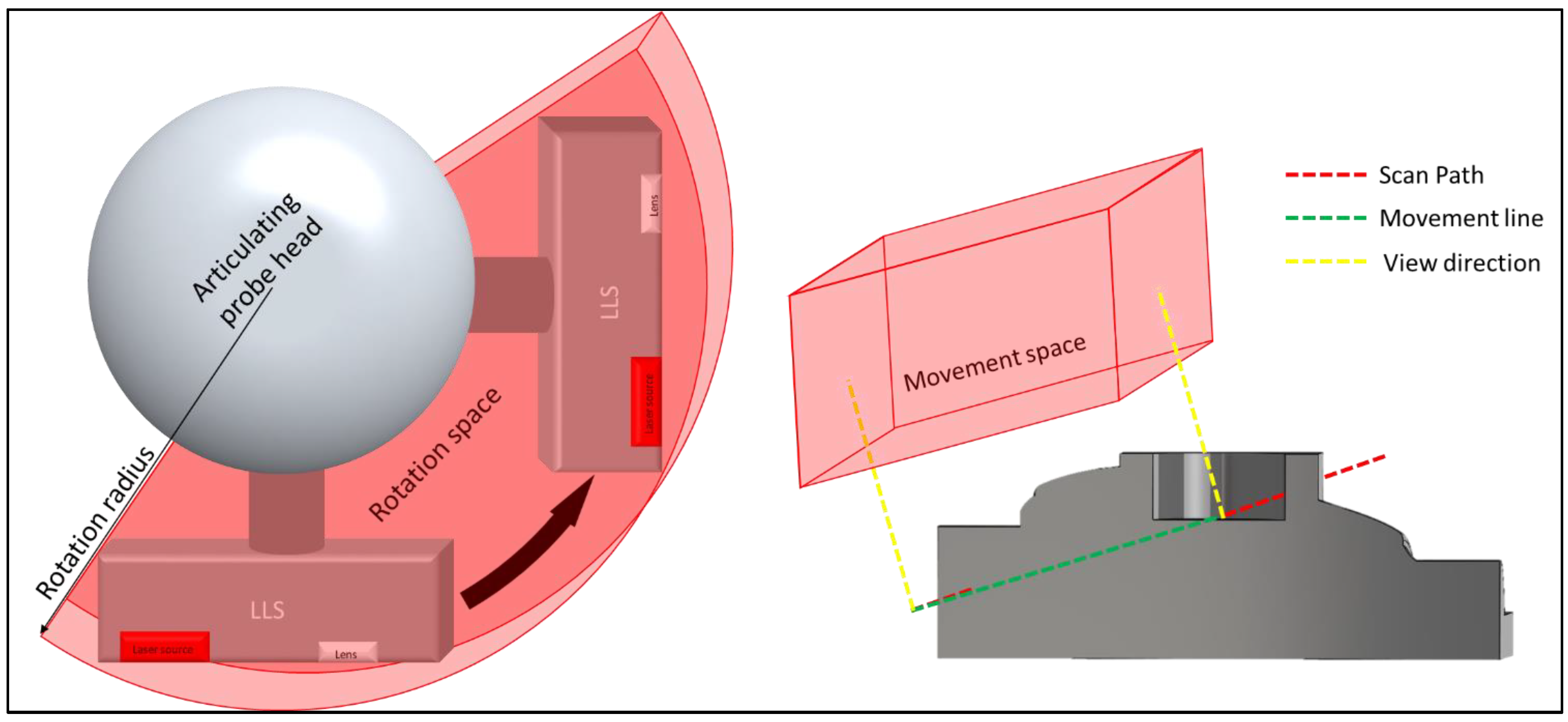
4.4. Step 4: Determine Scan Paths
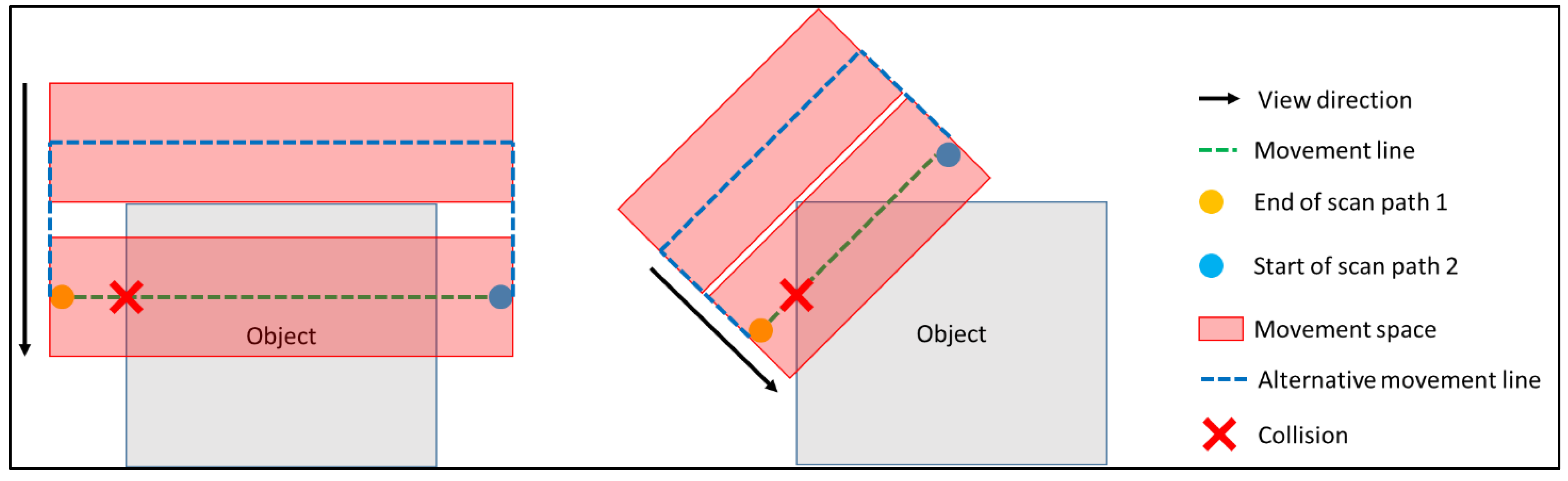
4.5. Step 5: Connect Scan Paths
4.6. Step 6: Measure Object
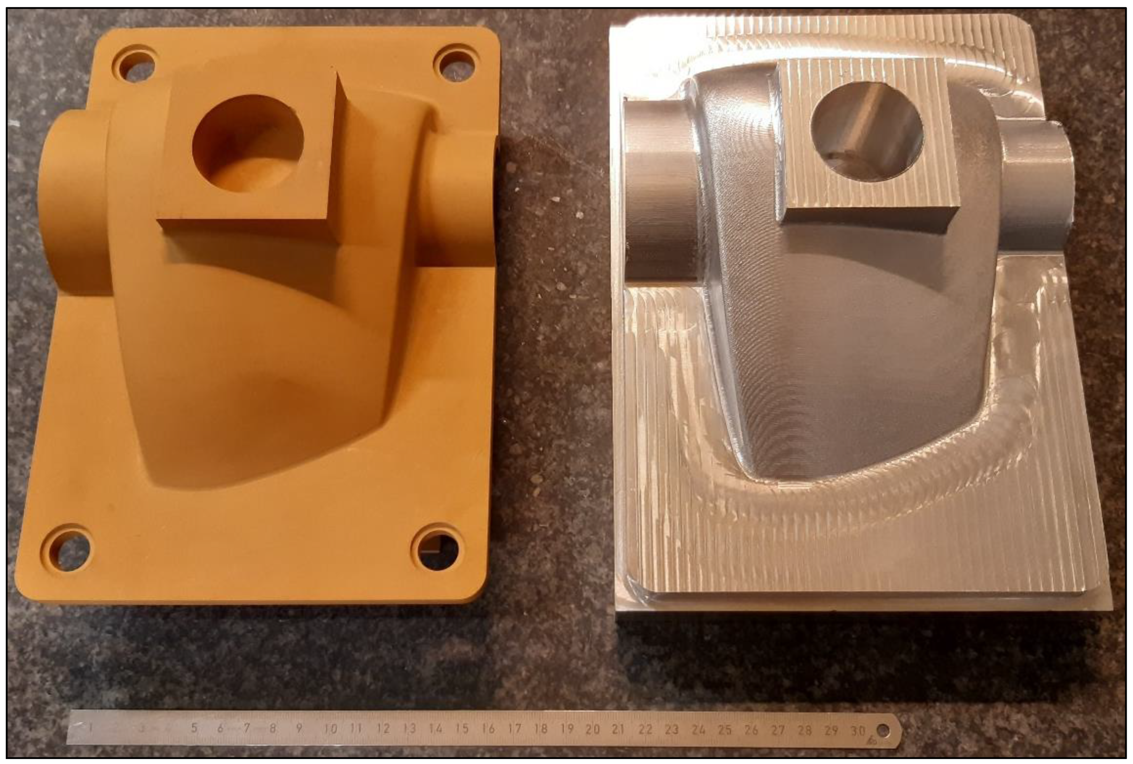
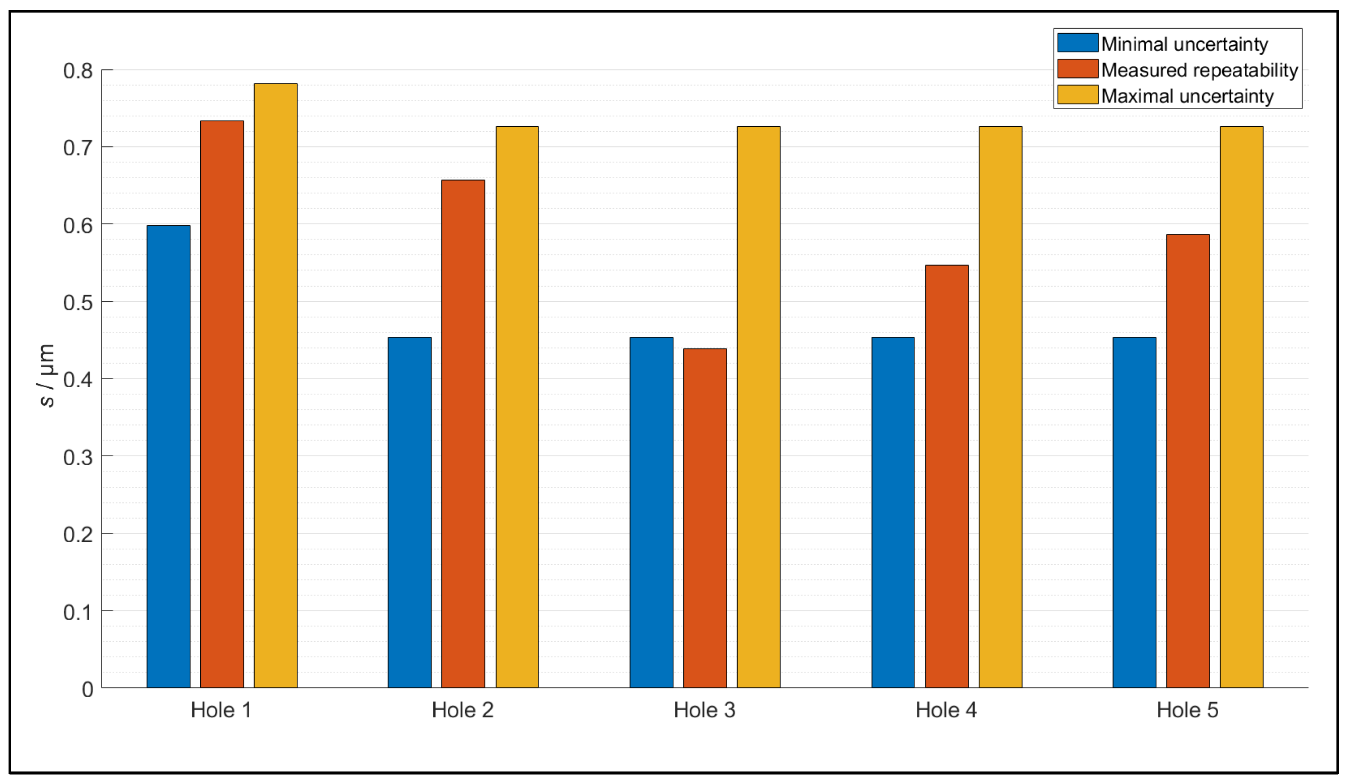
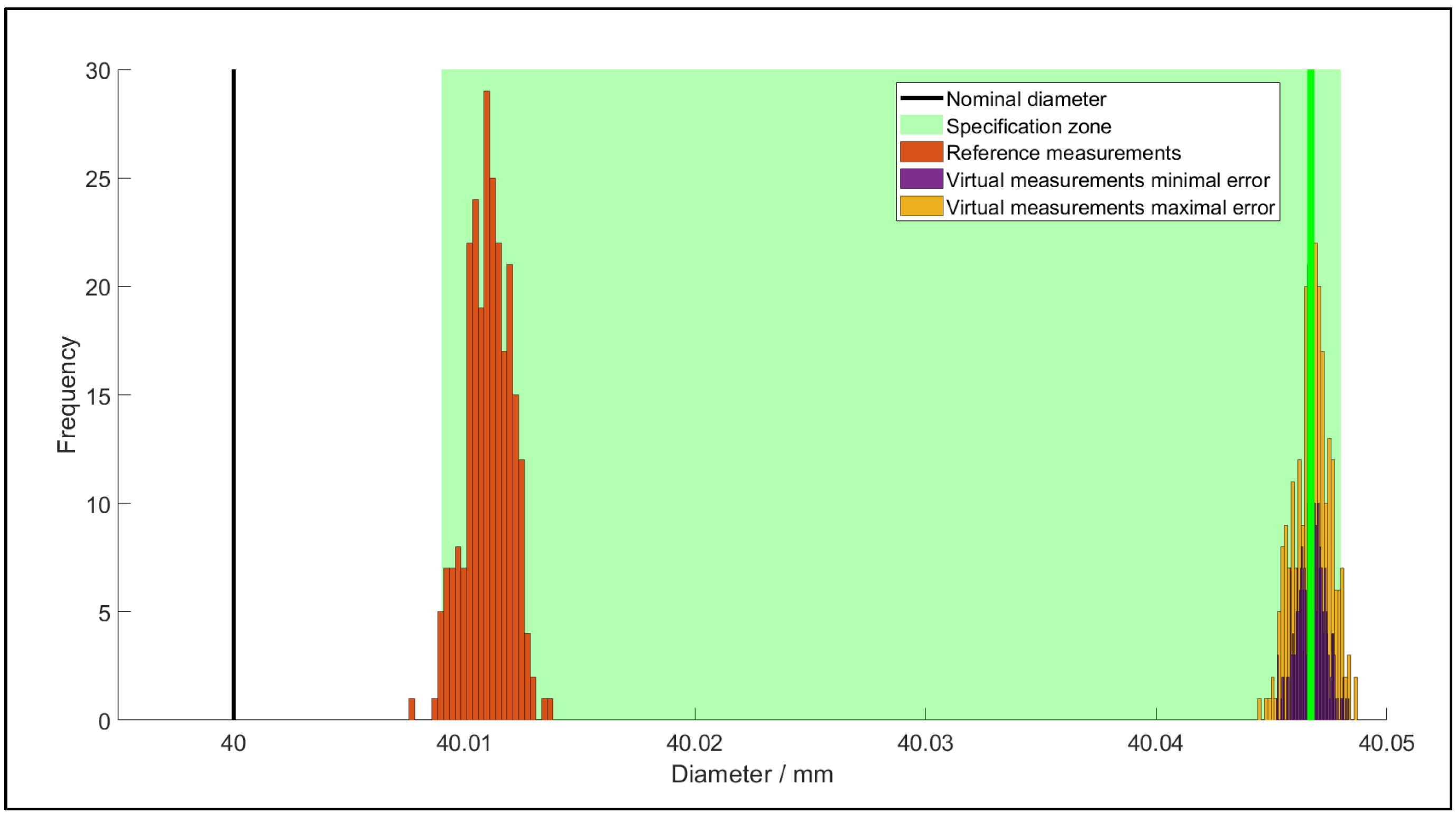
5. Validation
6. Conclusions
Author Contributions
Funding
Institutional Review Board Statement
Informed Consent Statement
Data Availability Statement
Conflicts of Interest
Appendix A

References
- Psarommatis, F.; Sousa, J.; Mendonça, J.P.; Kiritsis, D. Zero-defect manufacturing the approach for higher manufacturing sustainability in the era of industry 4.0: A position paper. Int. J. Prod. Res. 2022, 60, 73–91. [Google Scholar] [CrossRef]
- Imkamp, D.; Berthold, J.; Heizmann, M.; Kniel, K.; Manske, E.; Peterek, M.; Schmitt, R.; Seidler, J.; Sommer, K.-D. Challenges and trends in manufacturing measurement technology-the “Industrie 4.0” concept. J. Sensors Sens. Syst. 2016, 5, 325–335. [Google Scholar] [CrossRef] [Green Version]
- Kiraci, E.; Franciosa, P.; Turley, G.A.; Olifent, A.; Attridge, A.; Williams, M.A. Moving towards in-line metrology: Evaluation of a Laser Radar system for in-line dimensional inspection for automotive assembly systems. Int. J. Adv. Manuf. Technol. 2017, 91, 69–78. [Google Scholar] [CrossRef] [Green Version]
- Martins, F.A.R.; García-Bermejo, J.G.; Casanova, E.Z.; González, J.R.P. Automated 3D surface scanning based on CAD model. Mechatronics 2015, 15, 837–857. [Google Scholar] [CrossRef]
- Haitjema, H.; Morel, M.A.A. Noise bias removal in profile measurements. Measurement 2005, 38, 21–29. [Google Scholar] [CrossRef]
- Bos, E.J.C.; Delbressinge, F.L.M.; Haitjema, H. High-accuracy CMM metrology for micro systems. VDI Ber. 2004, 1860, 511–522. [Google Scholar]
- Mendrok, K.; Dworakowski, Z.; Dziedziech, K.; Holak, K. Indirect Measurement of Loading Forces with High-Camera. Sensors 2021, 21, 6643. [Google Scholar] [CrossRef]
- Scislo, L. Quality Assurance and Control of Steel Blade Production Using Full Non-Contact Frequency Response Analysis and 3D Laser Doppler Scanning Vibrometry System. In Proceedings of the 2021 11th IEEE International Conference on Intelligent Data Acquisition and Advanced Computing Systems: Technology and Applications (IDAACS), Cracow, Poland, 22–25 September 2021; Volume 11, pp. 419–423. [Google Scholar] [CrossRef]
- Abdulqader, A.; Rizos, D.C. Advantages of using digital image correlation techniques in uniaxial compression tests. Results Eng. 2020, 6, 100109. [Google Scholar] [CrossRef]
- Peuzin-Jubert, M.; Polette, A.; Nozais, D.; Mari, J.L.; Pernot, J.P. Survey on the View Planning Problem for Reverse Engineering and Automated Control Applications. Comput.-Aided Des. 2021, 141, 103094. [Google Scholar] [CrossRef]
- Xi, F.; Shu, C. CAD-based path planning for 3-D line laser scanning. Comput.-Aided Des. 1999, 31, 473–479. [Google Scholar] [CrossRef]
- Fernández, P.; Rico, J.C.; Álvarez, B.J.; Valiño, G.; Mateos, S. Laser scan planning based on visibility analysis and space partitioning techniques. Int. J. Adv. Manuf. Technol. 2008, 39, 699–715. [Google Scholar] [CrossRef]
- Boeckmans, B.; Zhang, M.; Welkenhuyzen, F.; Kruth, J.-P. Comparison of aspect ratio, accuracy and repeatability of a laser line scanning probe and a tactile probe. Laser Metrol. Precis. Meas. Insp. Ind. 2014, 9, 65–70. [Google Scholar] [CrossRef]
- Boeckmans, B.; Tan, Y.; Welkenhuyzen, F.; Guo, Y.; Dewulf, W.; Kruth, J.-P. Roughness offset differences between contact and non-contact measurements. In Proceedings of the 15th International Conference of the European Society for Precision Engineering and Nanotechnology, Leuven, Belgium, 1–5 June 2015; Volume 15, pp. 189–190. [Google Scholar]
- Son, S.; Park, H.; Lee, K.H. Automated laser scanning system for reverse engineering and inspection. Int. J. Adv. Manuf. Technol. 2002, 42, 889–897. [Google Scholar] [CrossRef]
- Wright, L.; Davidson, S. How to tell the diference between a model and a digital twin. Adv. Modeling Simul. Eng. Sci. 2020, 7, 1–13. [Google Scholar] [CrossRef]
- Vlaeyen, M.; Haitjema, H.; Dewulf, W. Digital Twin of an Optical Measurement System. Sensors 2021, 21, 6638. [Google Scholar] [CrossRef]
- ISO 14253-1: 2017; Geometrical Product specifications (GPS)—Inspection by Measurement of Workpieces and Measuring Equipment—Part 1: Decision Rules for Verifying Conformity or Nonconformity with Specifications, 1st ed. ISO: Geneva, Switzerland, 2017.
- Carmignato, S. Experimental study on performance verification tests for coordinate measuring systems with optical distance sensors. Proc SPIE—Int. Soc. Opt. Eng. 2009, 7239, 72390I. [Google Scholar] [CrossRef]
- Vlaeyen, M.; Haitjema, H.; Dewulf, W. Task-specific uncertainty determination by a digital twin. Precis. Eng. 2022. submitted. [Google Scholar]
- Tarbox, G.H.; Gottschlich, S.N. Planning for Complete Sensor Coverage in Inspection. Comput. Vis. Image Underst. 1995, 61, 84–111. [Google Scholar] [CrossRef]
- Lee, K.H.; Park, H. Automated inspection planning of free-form shape parts by laser scanning. Rob. Comput.-Integr. Manuf. 2000, 16, 201–210. [Google Scholar] [CrossRef]
- Lee, K.H.; Park, H.; Son, S. A Framework for Laser Scan Planning of Freeform Surfaces. Int. J. Adv. Manuf. Technol 2001, 17, 171–180. [Google Scholar] [CrossRef]
- Son, S.; Lee, K.H. Automated Scan Plan Generation Using STL Meshes for 3D Stripe-Type Laser Scanner. In International Conference on Computational Science and Its Applications; Springer: Berlin, Germany, 2003; pp. 741–750. [Google Scholar] [CrossRef]
- Son, S.; Kim, S.; Lee, K.H. Path planning of multi-patched freeform surfaces for laser scanning. Int. J. Adv. Manuf. Technol. 2003, 22, 424–435. [Google Scholar] [CrossRef]
- Ding, L.; Dai, S.; Mu, P. CAD-Based Path Planning for 3D Laser Scanning of Complex Surface. Procedia Comput. Sci. 2016, 92, 526–535. [Google Scholar] [CrossRef] [Green Version]
- Magaña, A.; Vlaeyen, M.; Haitjema, H.; Bauer, P.; Reinhart, G. Viewpoint Planning using Feature Cluster Constrained Spaces. ISPRS J. Photogramm. Remote Sens. 2022. submitted. [Google Scholar]
- Sadaoui, S.E.; Mehdi-Souzani, C.; Lartigue, C. Computer-Aided Inspection Planning: A Multisensor High-Level Inspection Planning Strategy. J. Comput. Inf. Sci. Eng. 2019, 19, 021005. [Google Scholar] [CrossRef]
- Zhao, H.; Kruth, J.-P.; Van Gestel, N.; Boeckmans, B.; Bleys, P. Automated dimensional inspection planning using the combination of laser scanner and tactile probe. Measurement 2012, 45, 1057–1066. [Google Scholar] [CrossRef] [Green Version]
- Mahmud, M.; Joannic, D.; Roy, M.; Isheil, A.; Fontaine, J.-F. 3D part inspection path planning of a laser scanner with control on the uncertainty. Comput.-Aided Des. 2011, 43, 345–355. [Google Scholar] [CrossRef]
- Phan, N.D.M.; Quinsat, Y.; Lartigue, C. Optimal scanning strategy for on-machine inspection with laser-plane sensor. Int. J. Adv. Manuf. Technol. 2019, 103, 4563–4576. [Google Scholar] [CrossRef] [Green Version]
- Sadaoui, E.S.; Mehdi-Souzani, C.; Lartigue, C.; Brahim, M. Automatic path planning for high performance measurement by laser plane sensors. Opt. Lasers Eng. 2022, 159, 107194. [Google Scholar] [CrossRef]
- Phan, N.D.M.; Quinsat, Y.; Lavernhe, S.; Lartigue, C. Scanner path planning with the control of overlap for part inspection with an industrial robot. Int. J. Adv. Manuf. Technol. 2018, 98, 629–643. [Google Scholar] [CrossRef]
- Glorieux, E.; Franciosa, P.; Ceglarek, D. Coverage path planning with targeted viewpoint sampling for robotic free-form surface inspection. Robot. Comput.-Integr. Manuf. 2020, 61, 101843. [Google Scholar] [CrossRef]


| Feature | Diameter Hole 1 | Diameter Hole 2 | Diameter Hole 3 | Diameter Hole 4 | Diameter Hole 5 | Distance between Planes |
|---|---|---|---|---|---|---|
| Nominal value/mm | 40 | 15 | 15 | 15 | 15 | 20 |
| Tolerance | G8 | H5 | H5 | H5 | H5 | m |
| Reference value/mm | 40.011 | 15.004 | 14.999 | 14.991 | 15.001 | 20.160 |
| 95% confidence interval/mm (reference) | [40.009; 40.013] | [15.032; 15.037] | [14.977; 14.982] | [14.949; 14.954] | [14.999; 15.004] | [20.158; 20.161] |
| Measured value/mm | 40.047 | 15.007 | 15.006 | 15.006 | 15.007 | 20.162 |
| 95% confidence interval/mm (experimental) | [40.045; 40.048] | [15.006; 15.008] | [15.005; 15.007] | [15.005; 15.007] | [15.006; 15.008] | [20.161; 20.164] |
| 95% minimal confidence interval/mm (virtual) | [40.046; 40.048] | [15.006; 15.008] | [15.005; 15.007] | [15.005; 15.007] | [15.006; 15.008] | [20.162; 20.163] |
| 95% maximal confidence interval/mm (virtual) | [40.045; 40.048] | [15.006; 15.009] | [15.005; 15.008] | [15.005; 15.008] | [15.006; 15.008] | [20.161; 20.164] |
| Conformance probability | 95% | 89% | 99% | 99% | 93% | 100% |
Publisher’s Note: MDPI stays neutral with regard to jurisdictional claims in published maps and institutional affiliations. |
© 2022 by the authors. Licensee MDPI, Basel, Switzerland. This article is an open access article distributed under the terms and conditions of the Creative Commons Attribution (CC BY) license (https://creativecommons.org/licenses/by/4.0/).
Share and Cite
Vlaeyen, M.; Haitjema, H.; Dewulf, W. Uncertainty-Based Autonomous Path Planning for Laser Line Scanners. Metrology 2022, 2, 479-494. https://doi.org/10.3390/metrology2040028
Vlaeyen M, Haitjema H, Dewulf W. Uncertainty-Based Autonomous Path Planning for Laser Line Scanners. Metrology. 2022; 2(4):479-494. https://doi.org/10.3390/metrology2040028
Chicago/Turabian StyleVlaeyen, Michiel, Han Haitjema, and Wim Dewulf. 2022. "Uncertainty-Based Autonomous Path Planning for Laser Line Scanners" Metrology 2, no. 4: 479-494. https://doi.org/10.3390/metrology2040028