
Key Epidemic Parameters of the SIRV Model Determined from Past COVID-19 Mutant Waves


Abstract
:1. Introduction
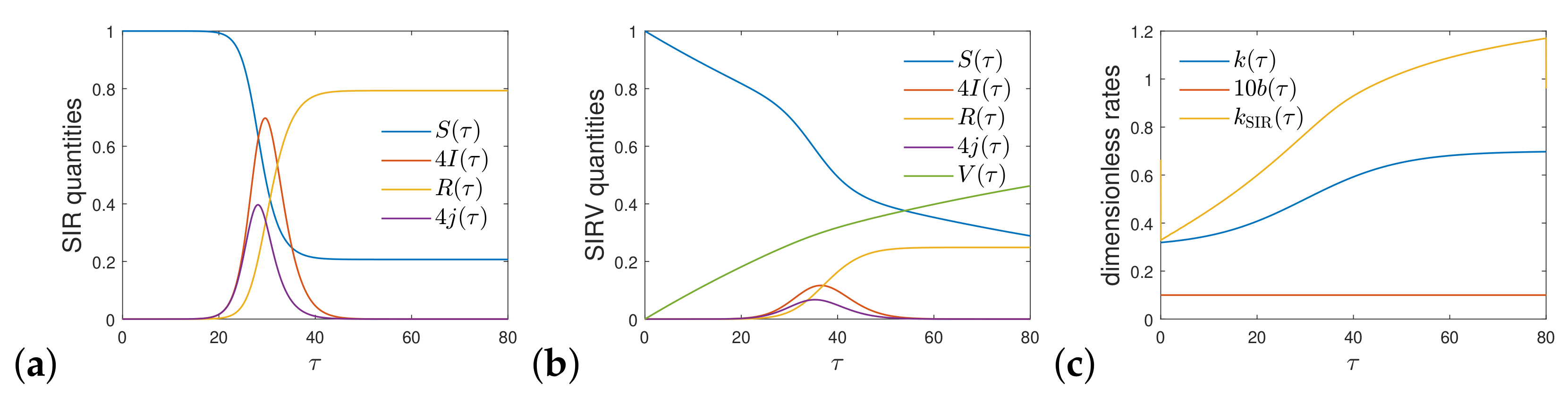
2. SIRV Model
2.1. Starting Equations
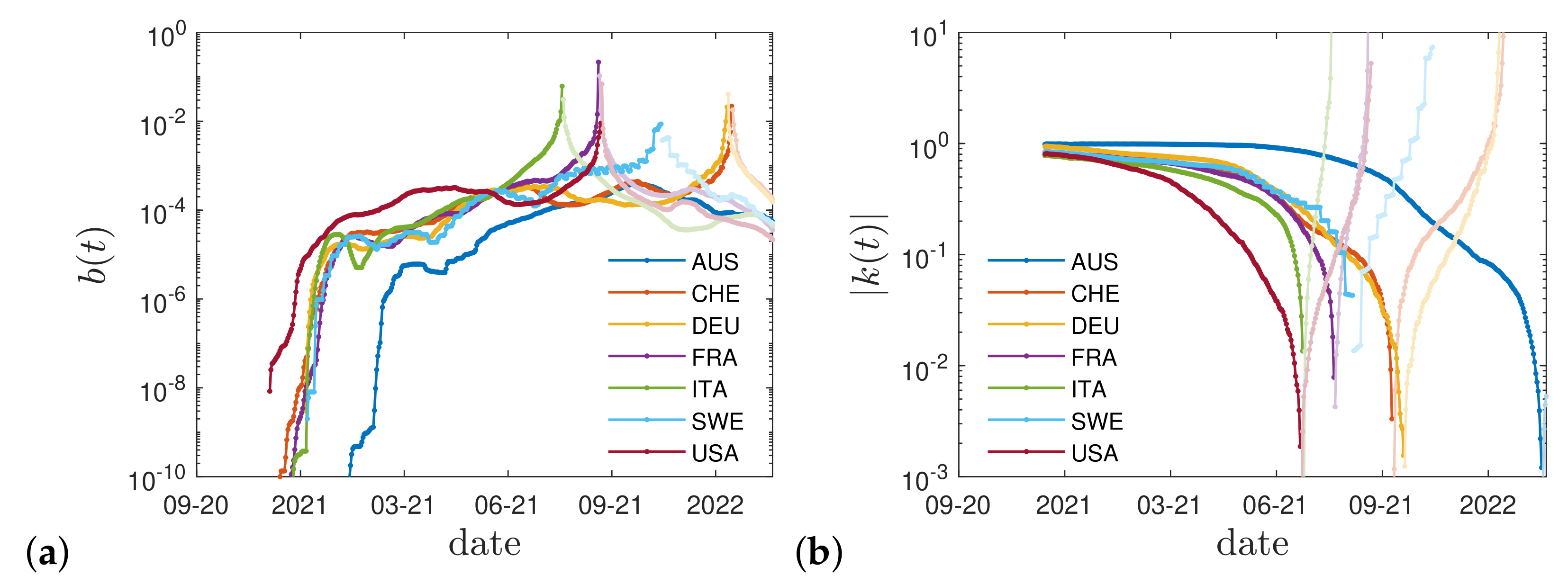
2.2. Key Parameter
2.3. Comparison with the SIR Model Limit
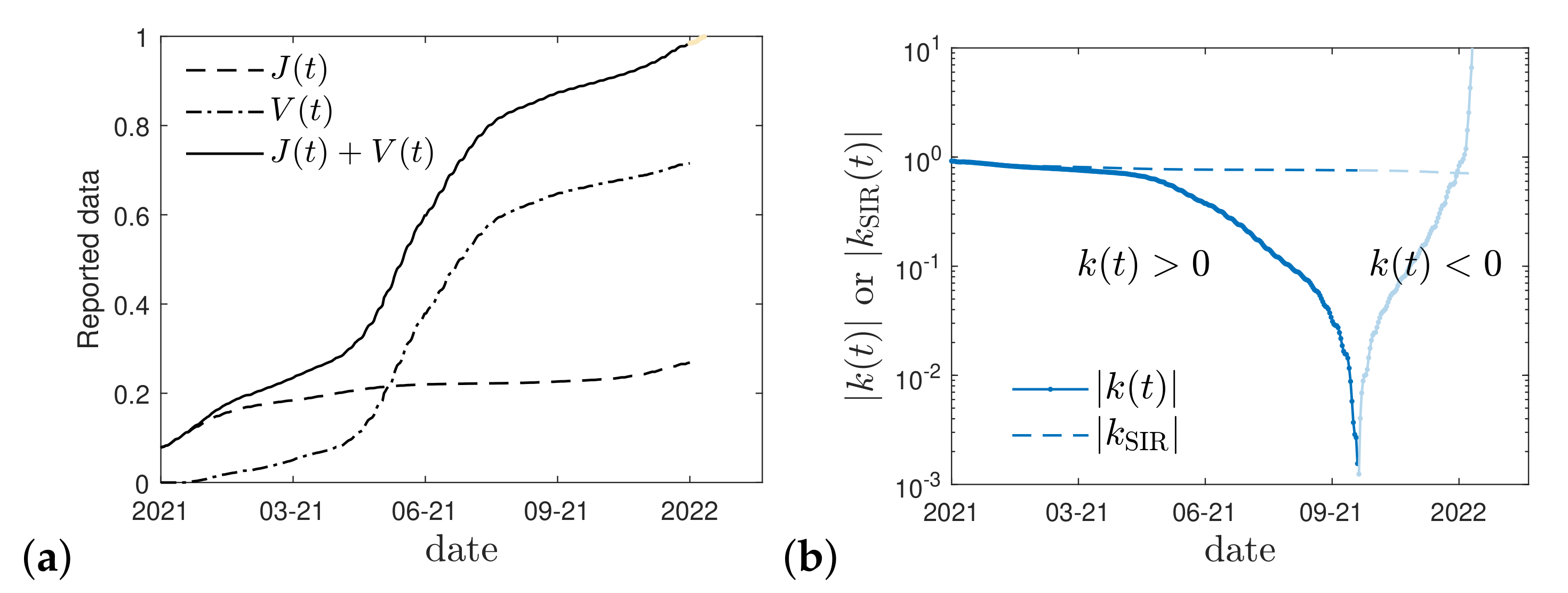
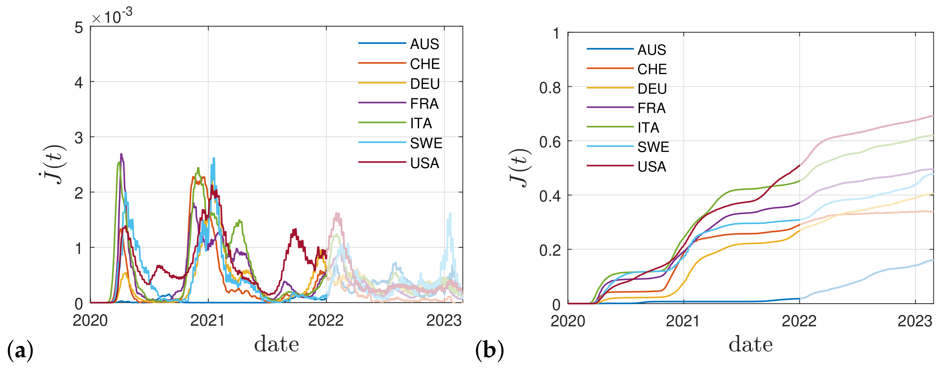
2.4. Real Time Dependence
3. Cumulative Vaccination Fraction
4. Conclusions
Author Contributions
Funding
Informed Consent Statement
Data Availability Statement
Conflicts of Interest
References
- Schlickeiser, R.; Kröger, M. Analytical modeling of the temporal evolution of epidemics outbreaks accounting for vaccinations. Physics 2021, 3, 386–426. [Google Scholar] [CrossRef]
- Babaei, N.A.; Ozer, T. On exact integrability of a COVID-19 model: SIRV. Math. Meth. Appl. Sci. 2023, 1, 1–18. [Google Scholar] [CrossRef]
- Rifhat, R.; Teng, Z.; Wang, C. Extinction and persistence of a stochastic SIRV epidemic model with nonlinear incidence rate. Adv. Diff. Eqs. 2021, 2021, 200. [Google Scholar] [CrossRef]
- Ameen, I.; Baleanu, D.; Ali, H.M. An efficient algorithm for solving the fractional optimal control of SIRV epidemic model with a combination of vaccination and treatment. Chaos Solit. Fract. 2020, 137, 109892. [Google Scholar] [CrossRef]
- Oke, M.O.; Ogunmiloro, O.M.; Akinwumi, C.T.; Raji, R.A. Mathematical Modeling and Stability Analysis of a SIRV Epidemic Model with Non-linear Force of Infection and Treatment. Commun. Math. Appl. 2019, 10, 717–731. [Google Scholar] [CrossRef] [Green Version]
- Kermack, W.O.; McKendrick, A.G. A contribution to the mathematical theory of epidemics. Proc. R. Soc. A 1927, 115, 700. [Google Scholar] [CrossRef] [Green Version]
- Kendall, D.G. Deterministic and stochastic epidemics in closed populations. In Proceedings of the Third Berkeley Symposium on Mathematical Statistics and Probability, Berkeley, CA, USA, 1 January 1956; Volume 4, pp. 149–165. [Google Scholar] [CrossRef]
- Postnikov, E.B. Estimation of COVID-19 dynamics “on a back-of-envelope”: Does the simplest SIR model provide quantitative parameters and predictions? Chaos Solit. Fract. 2020, 135, 109841. [Google Scholar] [CrossRef]
- Cooper, I.; Mondal, A.; Antonopoulos, C.G. A SIR model assumption for the spread of COVID-19 in different communities. Chaos Solit. Fract. 2020, 139, 110057. [Google Scholar] [CrossRef]
- Hespanha, J.P.; Chinchilla, R.; Costa, R.R.; Erdal, M.K.; Yang, G. Forecasting COVID-19 cases based on a parameter-varying stochastic SIR model. Annu. Rev. Control 2021, 51, 460–476. [Google Scholar] [CrossRef]
- Annas, S.; Pratama, M.I.; Rifandi, M.; Sanusi, W.; Side, S. Stability analysis and numerical simulation of SEIR model for pandemic COVID-19 spread in Indonesia. Chaos Solit. Fract. 2020, 139, 110072. [Google Scholar] [CrossRef]
- Hou, C.; Chen, J.; Zhou, Y.; Hua, L.; Yuan, J.; He, S.; Guo, Y.; Zhang, S.; Jia, Q.; Zhao, C.; et al. The effectiveness of quarantine of Wuhan city against the Corona Virus Disease 2019 (COVID-19): A well-mixed SEIR model analysis. J. Med. Virol. 2020, 92, 841–848. [Google Scholar] [CrossRef] [PubMed] [Green Version]
- Yang, Z.; Zeng, Z.; Wang, K.; Wong, S.S.; Liang, W.; Zanin, M.; Liu, P.; Cao, X.; Gao, Z.; Mai, Z.; et al. Modified SEIR and AI prediction of the epidemics trend of COVID-19 in China under public health interventions. J. Thorac. Dis. 2020, 12, 165. [Google Scholar] [CrossRef]
- He, S.; Peng, Y.; Sun, K. SEIR modeling of the COVID-19 and its dynamics. Nonlin. Dyn. 2020, 101, 1667–1680. [Google Scholar] [CrossRef] [PubMed]
- Rezapour, S.; Mohammadi, H.; Samei, M.E. SEIR epidemic model for COVID-19 transmission by Caputo derivative of fractional order. Adv. Diff. Eqs. 2020, 2020, 490. [Google Scholar] [CrossRef]
- Ghostine, R.; Gharamti, M.; Hassrouny, S.; Hoteit, I. An Extended SEIR Model with Vaccination for Forecasting the COVID-19 Pandemic in Saudi Arabia Using an Ensemble Kalman Filter. Mathematics 2021, 9, 636. [Google Scholar] [CrossRef]
- Berger, D.; Herkenhoff, K.; Huang, C.; Mongey, S. Testing and reopening in an SEIR model. Rev. Econ. Dyn. 2022, 43, 1–21. [Google Scholar] [CrossRef]
- Engbert, R.; Rabe, M.M.; Kliegl, R.; Reich, S. Sequential Data Assimilation of the Stochastic SEIR Epidemic Model for Regional COVID-19 Dynamics. Bull. Math. Biol. 2021, 83, 1. [Google Scholar] [CrossRef]
- Bentout, S.; Chen, Y.; Djilali, S. Global Dynamics of an SEIR Model with Two Age Structures and a Nonlinear Incidence. Acta Appl. Math. 2021, 171, 7. [Google Scholar] [CrossRef]
- Carcione, J.M.; Santos, J.E.; Bagaini, C.; Ba, J. A Simulation of a COVID-19 Epidemic Based on a Deterministic SEIR Model. Front. Publ. Health 2020, 8, 230. [Google Scholar] [CrossRef]
- Nabti, A.; Ghanbari, B. Global stability analysis of a fractional SVEIR epidemic model. Math. Meth. Appl. Sci. 2021, 44, 8577–8597. [Google Scholar] [CrossRef]
- Lopez, L.; Rodo, X. A modified SEIR model to predict the COVID-19 outbreak in Spain and Italy: Simulating control scenarios and multi-scale epidemics. Results Phys. 2021, 21, 103746. [Google Scholar] [CrossRef]
- Korolev, I. Identification and estimation of the SEIRD epidemic model for COVID-19. J. Econom. 2021, 220, 63–85. [Google Scholar] [CrossRef] [PubMed]
- Jahanshahi, H.; Munoz-Pacheco, J.M.; Bekiros, S.; Alotaibi, N.D. A fractional-order SIRD model with time-dependent memory indexes for encompassing the multi-fractional characteristics of the COVID-19. Chaos Solit. Fract. 2021, 143, 110632. [Google Scholar] [CrossRef] [PubMed]
- Nisar, K.S.; Ahmad, S.; Ullah, A.; Shah, K.; Alrabaiah, H.; Arfan, M. Mathematical analysis of SIRD model of COVID-19 with Caputo fractional derivative based on real data. Results Phys. 2021, 21, 103772. [Google Scholar] [CrossRef]
- Faruk, O.; Kar, S. A Data Driven Analysis and Forecast of COVID-19 Dynamics during the Third Wave Using SIRD Model in Bangladesh. Covid 2021, 1, 503–517. [Google Scholar] [CrossRef]
- Rajasekar, S.P.; Pitchaimani, M. Ergodic stationary distribution and extinction of a stochastic SIRS epidemic model with logistic growth and nonlinear incidence. Appl. Math. Comput. 2020, 377, 125143. [Google Scholar] [CrossRef]
- Hu, H.; Yuan, X.; Huang, L.; Huang, C. Global dynamics of an SIRS model with demographics and transfer from infectious to susceptible on heterogeneous networks. Math. Biosci. Eng. 2019, 16, 5729–5749. [Google Scholar] [CrossRef] [PubMed]
- Keeling, M.J.; Rohani, P. Modeling Infectious Diseases in Humans and Animals; Princeton University Press: Princeton, NJ, USA, 2008. [Google Scholar] [CrossRef] [Green Version]
- Estrada, E. COVID-19 and SARS-COV-2, Modeling the present, looking at the future. Phys. Rep. 2020, 869, 1. [Google Scholar] [CrossRef]
- Lopez, L.; Rodo, X. The end of social confinement and COVID-19 re-emergence risk. Nat. Hum. Behav. 2020, 4, 746–755. [Google Scholar] [CrossRef] [PubMed]
- Miller, I.F.; Becker, A.D.; Grenfell, B.T.; Metcalf, C.J.E. Disease and healthcare burden of COVID-19 in the United States. Nat. Med. 2020, 26, 1212–1217. [Google Scholar] [CrossRef]
- Reiner, R.C., Jr.; Barber, R.M.; Collins, J.K.; Zheng, P.; Adolph, C.; Albright, J.; Antony, C.M.; Aravkin, A.Y.; Bachmeier, S.D.; Bang-Jensen, B.; et al. Modeling COVID-19 scenarios for the United States. Nat. Med. 2021, 27, 94–105. [Google Scholar] [CrossRef]
- Linka, K.; Peirlinck, M.; Sahli Costabal, F.; Kuhl, E. Outbreak dynamics of COVID-19 in Europe and the effect of travel restrictions. Comp. Meth. Biomech. Biomed. Eng. 2020, 23, 710–717. [Google Scholar] [CrossRef] [PubMed]
- Filindassi, V.; Pedrini, C.; Sabadini, C.; Duradoni, M.; Guazzini, A. Impact of COVID-19 First Wave on Psychological and Psychosocial Dimensions: A Systematic Review. Covid 2022, 2, 273–340. [Google Scholar] [CrossRef]
- Schlickeiser, R.; Kröger, M. Determination of a key pandemic parameter of the SIR-epidemic model from past COVID-19 mutant waves and its variation for the validity of the Gaussian evolution. Physics 2023, 5, 205–214. [Google Scholar] [CrossRef]
- Schlickeiser, R.; Kröger, M. Reasonable limiting of 7-day incidence per hundred thousand value and herd immunization in Germany and other countries. Covid 2021, 1, 130–136. [Google Scholar] [CrossRef]
- Dong, E.; Du, H.; Gardner, L. An interactive web-based dashboard to track COVID-19 in real time. Lancet Infect. Dis. 2020, 20, 533–534. Available online: https://pomber.github.io/covid19/timeseries.json (accessed on 5 February 2023). [CrossRef] [PubMed]


| Country | Code | |||
|---|---|---|---|---|
| Australia | AUS | 570 | 78 days | 0.90 |
| Switzerland | CHE | 479 | 86 days | 0.72 |
| Germany | DEU | 491 | 83 days | 0.76 |
| France | FRA | 494 | 92 days | 0.80 |
| Italy | ITA | 492 | 88 days | 0.79 |
| Sweden | SWE | 503 | 85 days | 0.77 |
| United States | USA | 407 | 122 days | 0.70 |
Disclaimer/Publisher’s Note: The statements, opinions and data contained in all publications are solely those of the individual author(s) and contributor(s) and not of MDPI and/or the editor(s). MDPI and/or the editor(s) disclaim responsibility for any injury to people or property resulting from any ideas, methods, instructions or products referred to in the content. |
© 2023 by the authors. Licensee MDPI, Basel, Switzerland. This article is an open access article distributed under the terms and conditions of the Creative Commons Attribution (CC BY) license (https://creativecommons.org/licenses/by/4.0/).
Share and Cite
Schlickeiser, R.; Kröger, M. Key Epidemic Parameters of the SIRV Model Determined from Past COVID-19 Mutant Waves. COVID 2023, 3, 592-600. https://doi.org/10.3390/covid3040042
Schlickeiser R, Kröger M. Key Epidemic Parameters of the SIRV Model Determined from Past COVID-19 Mutant Waves. COVID. 2023; 3(4):592-600. https://doi.org/10.3390/covid3040042
Chicago/Turabian StyleSchlickeiser, Reinhard, and Martin Kröger. 2023. "Key Epidemic Parameters of the SIRV Model Determined from Past COVID-19 Mutant Waves" COVID 3, no. 4: 592-600. https://doi.org/10.3390/covid3040042