
Digitally Based Precision Time-Domain Spectrometer for NMR Relaxation and NMR Cryoporometry


Abstract
:1. Introduction
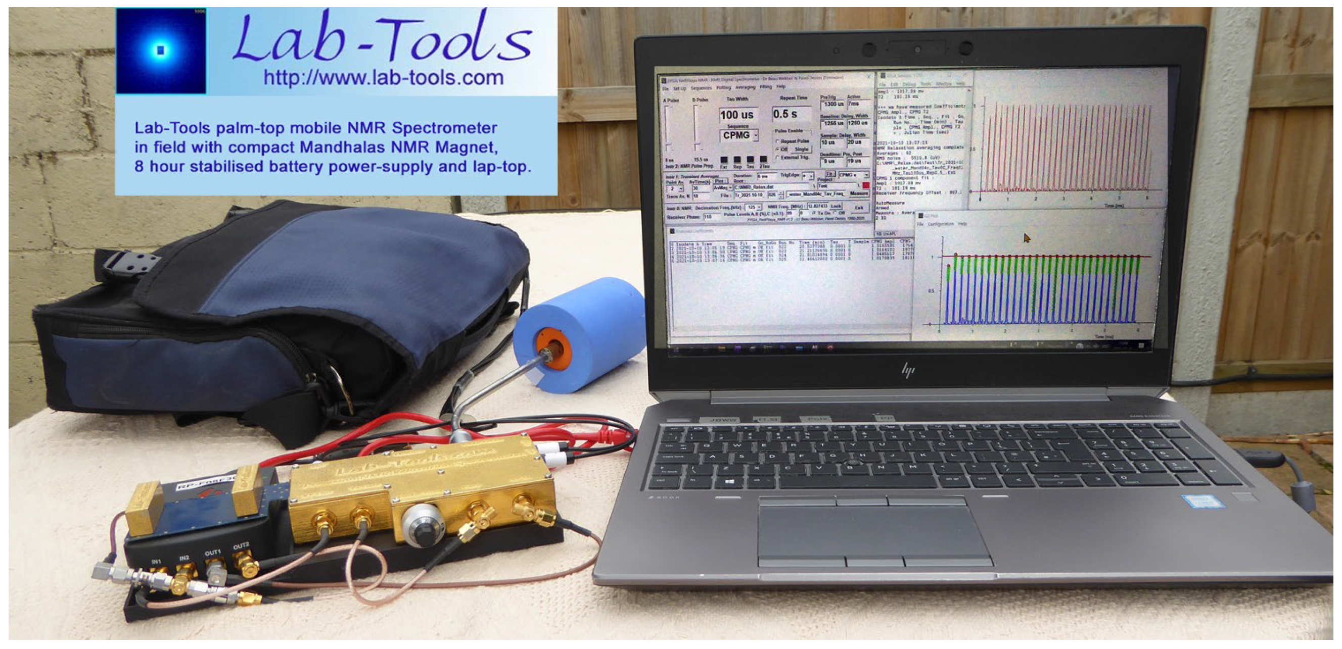
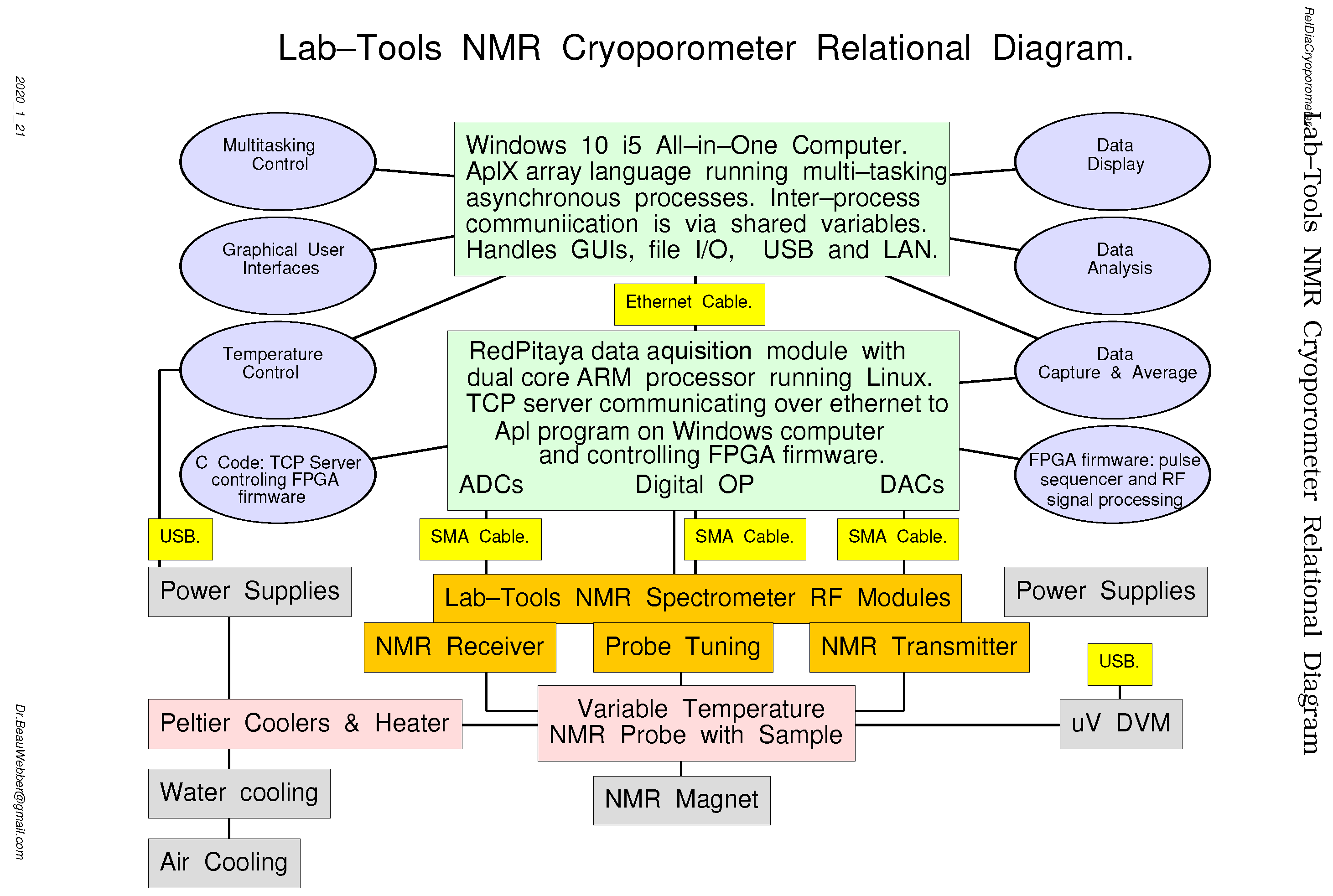
2. Lab-Tools Mk3 NMR Time-Domain Relaxation Spectrometer
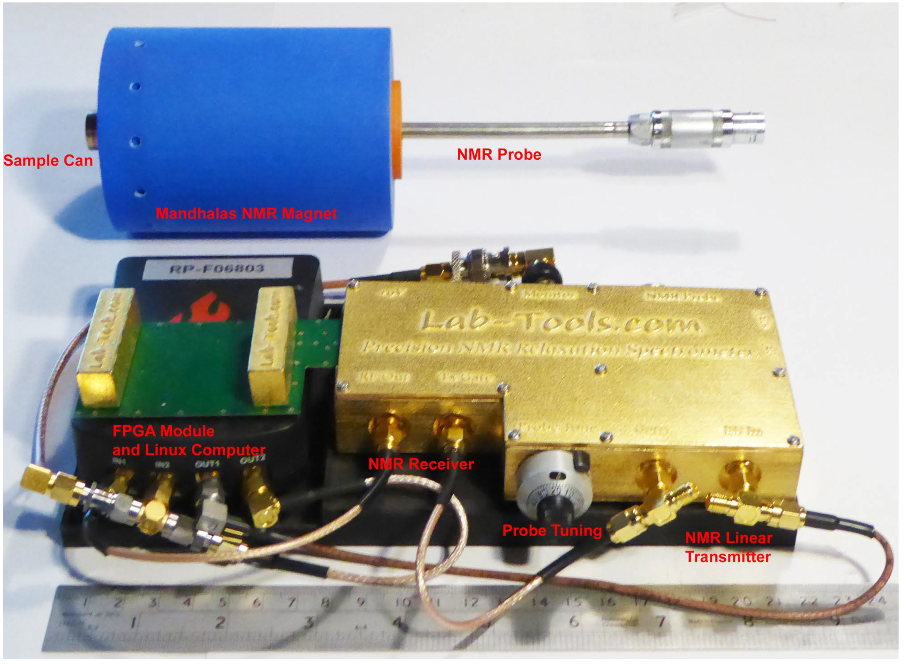
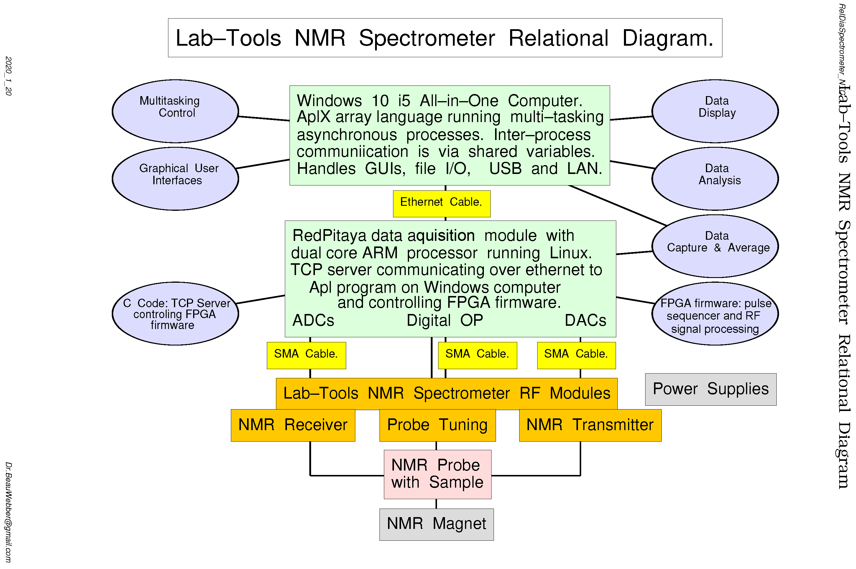
3. NMR Spectrometer Hardware
3.1. Data Acquisition Module
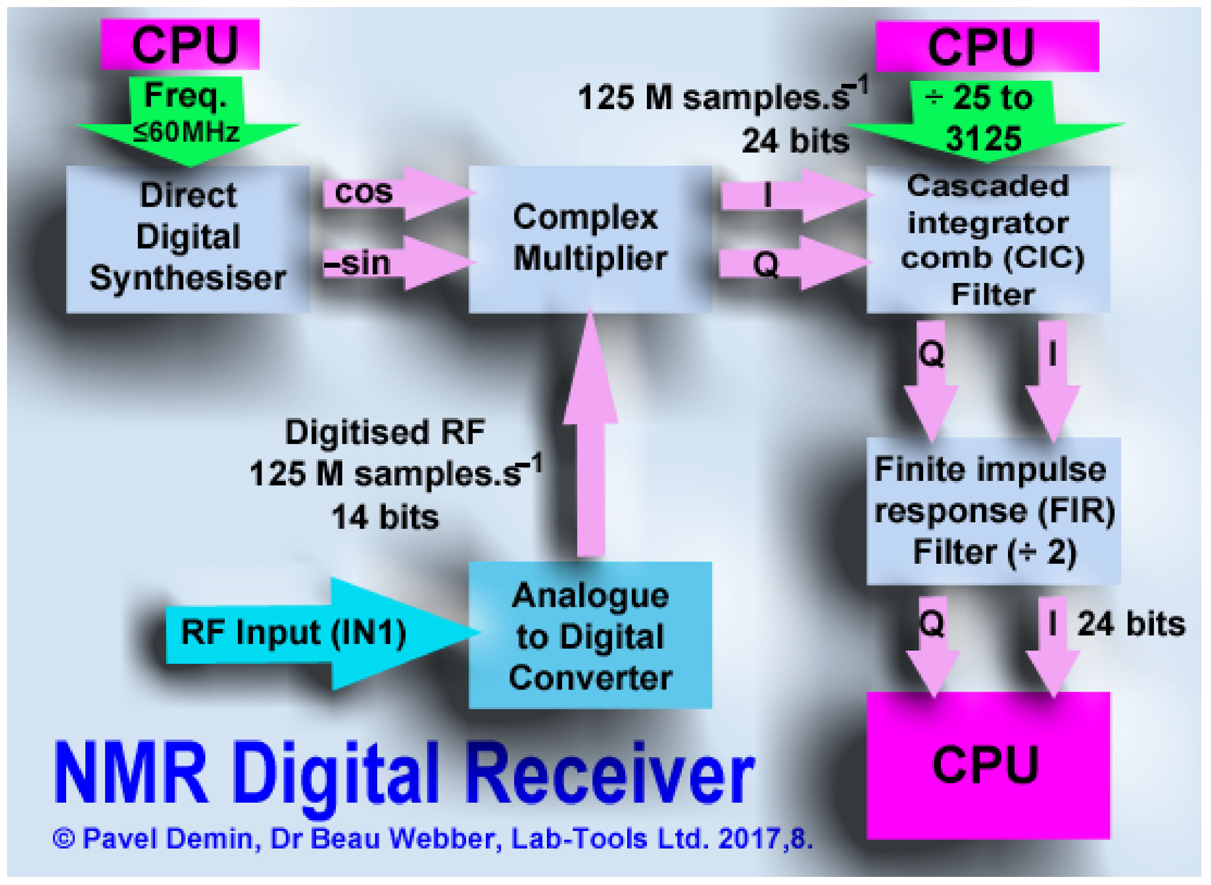
3.2. Receiver
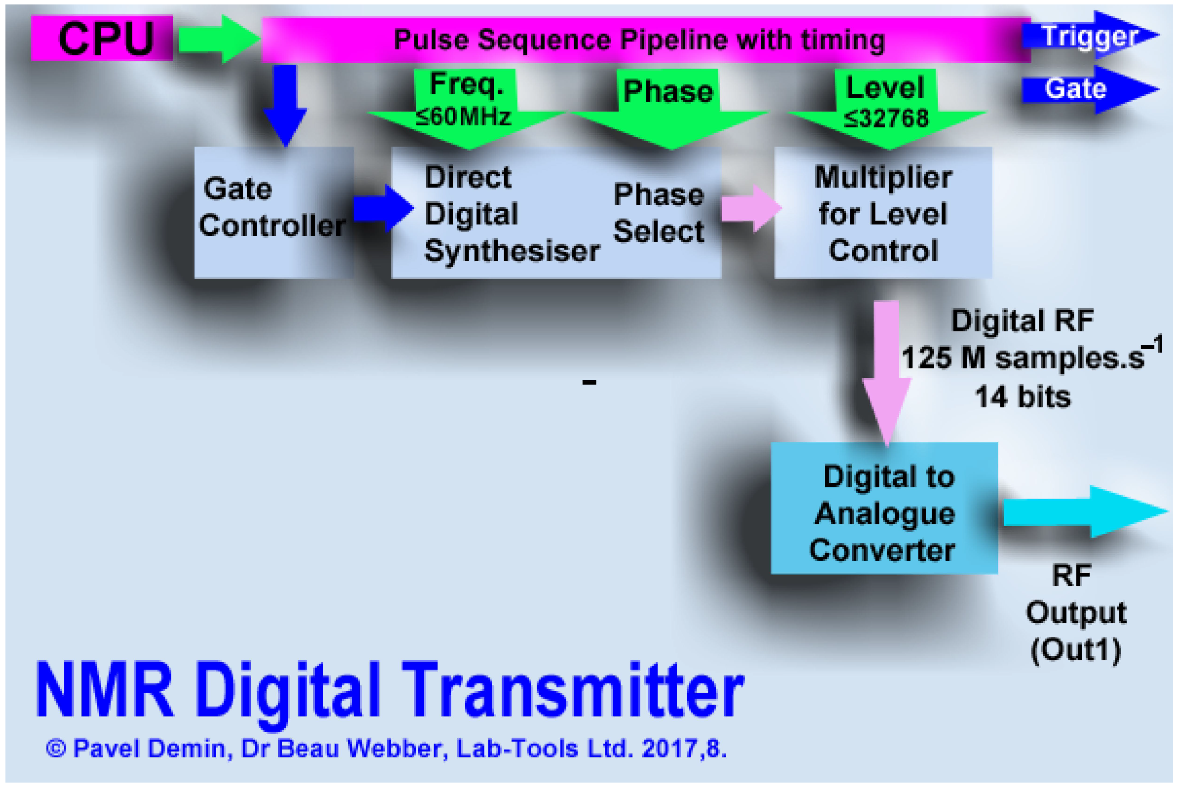
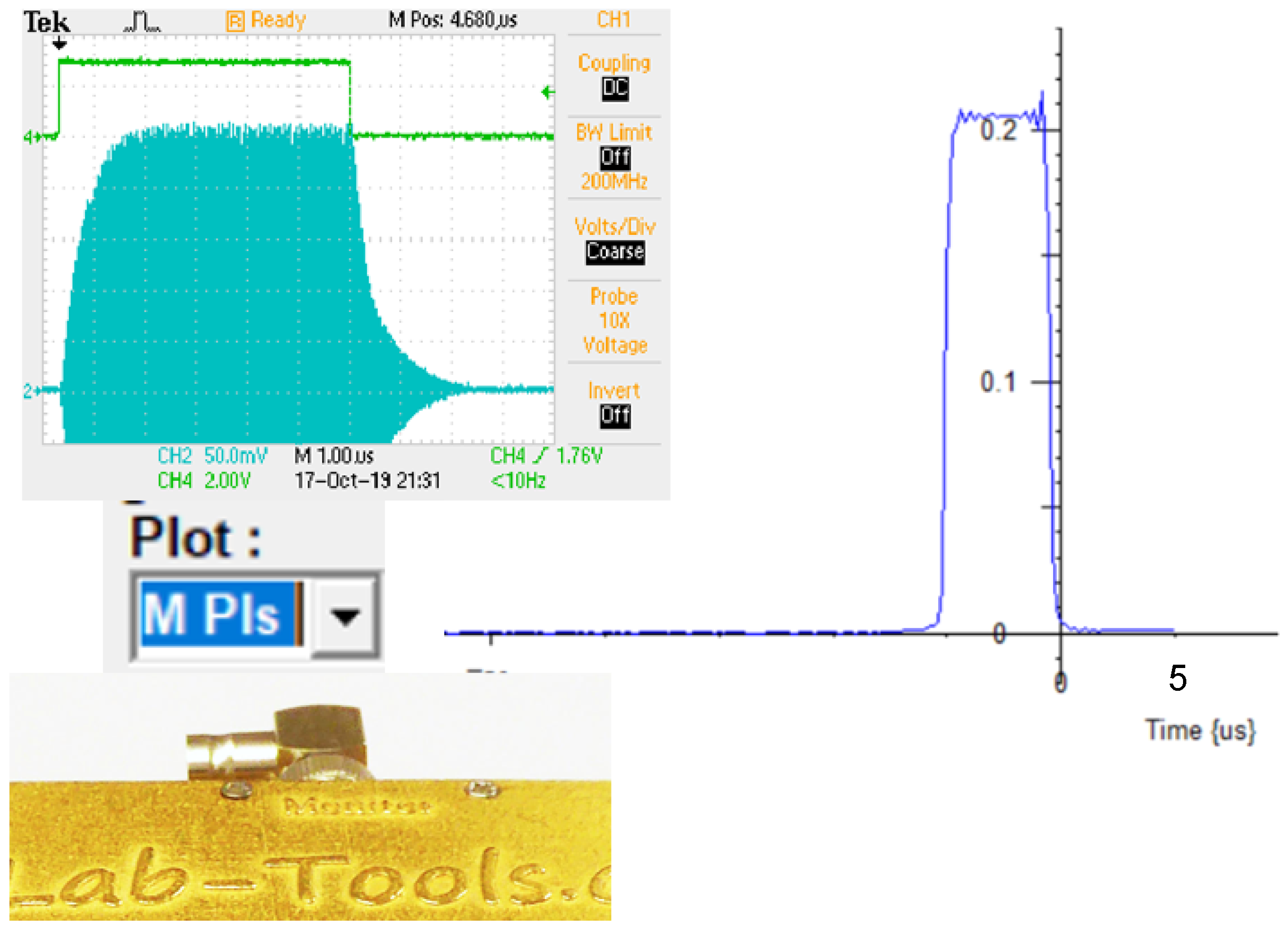
3.3. Transmitter
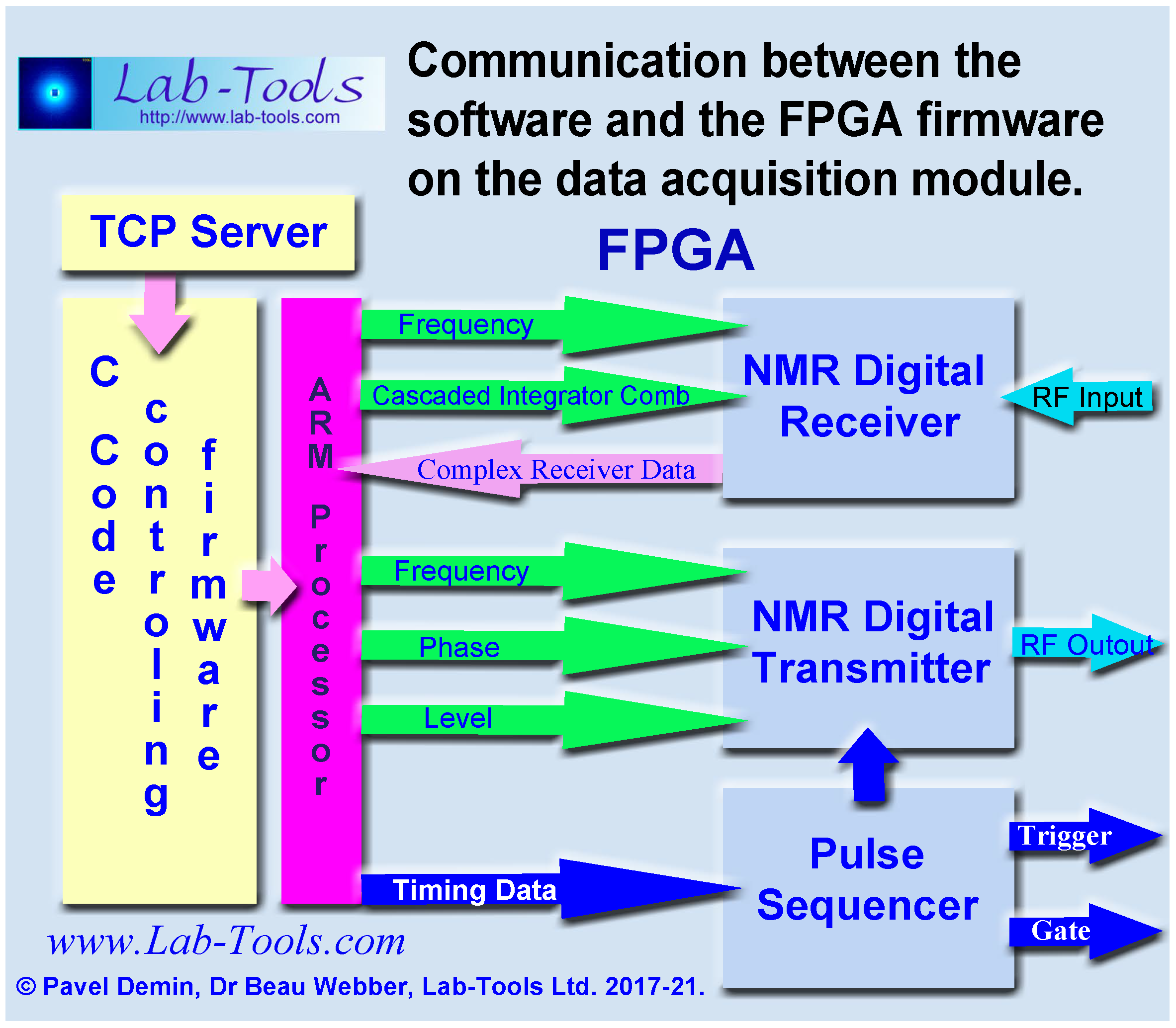
4. NMR Spectrometer Firmware
- Configuration registers;
- Status registers;
- Signal processing modules.
Digital Down-Converter
- A direct digital synthesizer (DDS) [46] generating a complex sinusoid;
- A complex multiplier based on the DSP48 modules [47];
- A CIC filter [48] used to decrease the sample rate by a configurable factor;
- An FIR filter [49] that compensates for the drop in the CIC frequency response and reduces the sample rate by a factor of two;
- A FIFO buffer storing the IQ samples before they are read by the CPU.
Pulse Generator
- A FIFO buffer storing the pulse parameters received from the CPU;
- A programmable gate controller;
- A direct digital synthesizer (DDS) [46];
- A multiplier controlling the amplitude of the output signal.
- Pulse duration (64 bits), expressed as a number of 8 ns clock pulses;
- Phase offset (32 bits), expressed in degrees;
- Pulse level (16 bits), expressed in arbitrary units from 0 to 32,766, with 32,766 corresponding to the maximum pulse level.
- Sets the DDS phase offset;
- Opens the gate controlling the data flow between the DDS and the DAC interface;
- Starts counting 8 ns clock pulses;
- Waits until the number of counted 8 ns clock pulses is equal to the pulse duration;
- Closes the gate.
5. NMR Spectrometer Software
- A TCP server running on the CPU of the data acquisition module;
- A TCP client .NET library implementing a minimalistic set of commands.
5.1. TCP Server
5.2. TCP client .NET Library
- Commands to manage the connection with the TCP server:
- -
- Connect(address);
- -
- Disconnect();
- Commands to set the frequencies and decimation rate:
- -
- SetFreqRX(frequency);
- -
- SetFreqTX(frequency);
- -
- SetRateRX(rate);
- Commands to program a pulse sequence:
- -
- ClearPulses();
- -
- AddDelay(duration);
- -
- AddPulse(level, phase, duration);
- Command to start pulse sequence and receive data:
- -
- RecieveData(size);
- Various commands to control output RF signal level, GPIO pins and receiver RF amplifier gain:
- -
- SetLevelTX(level);
- -
- SetPin(pin);
- -
- ClearPin(pin);
- -
- SetDAC(data).
5.3. High-Level Programming of the NMR Pulse Sequences
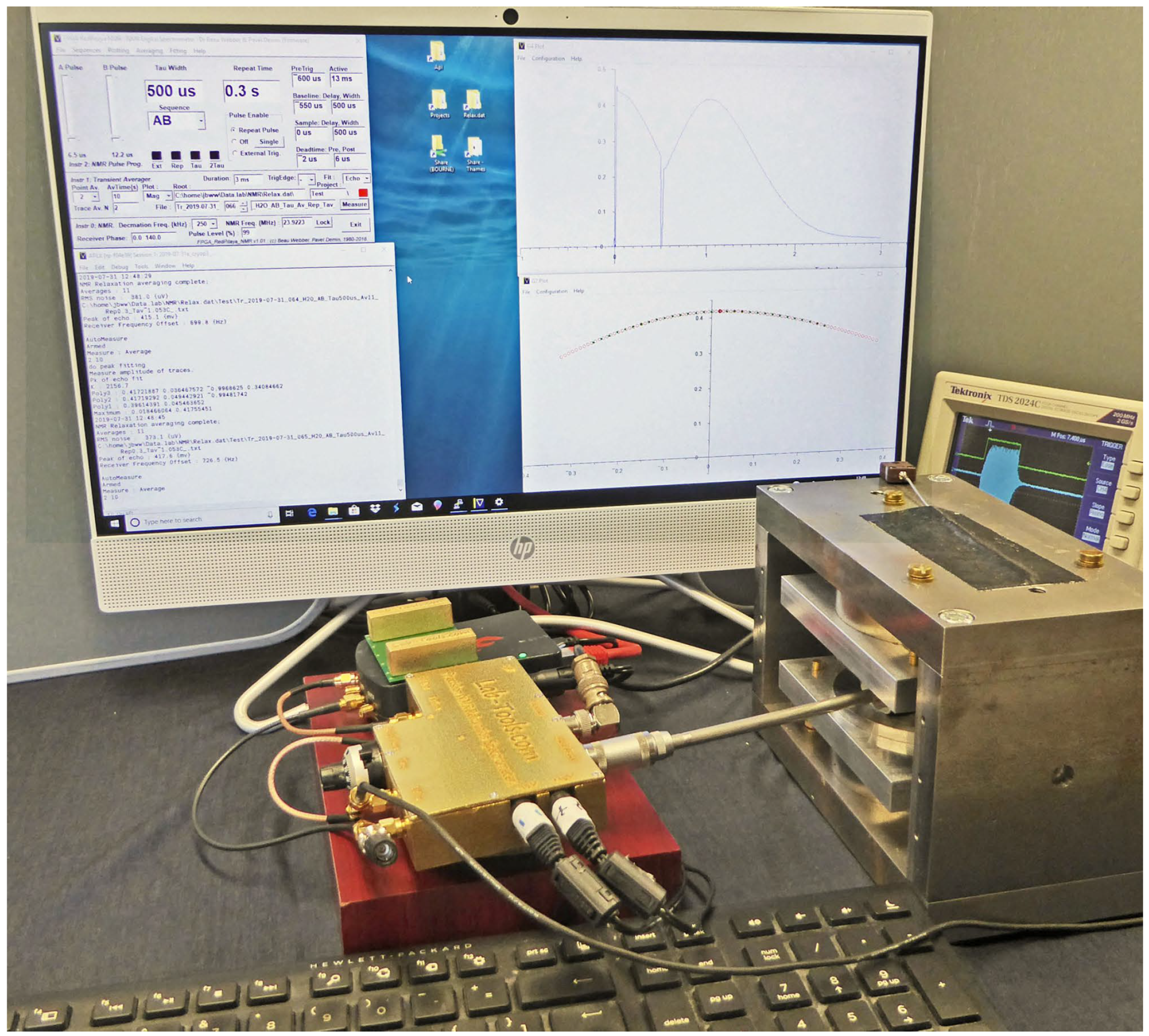
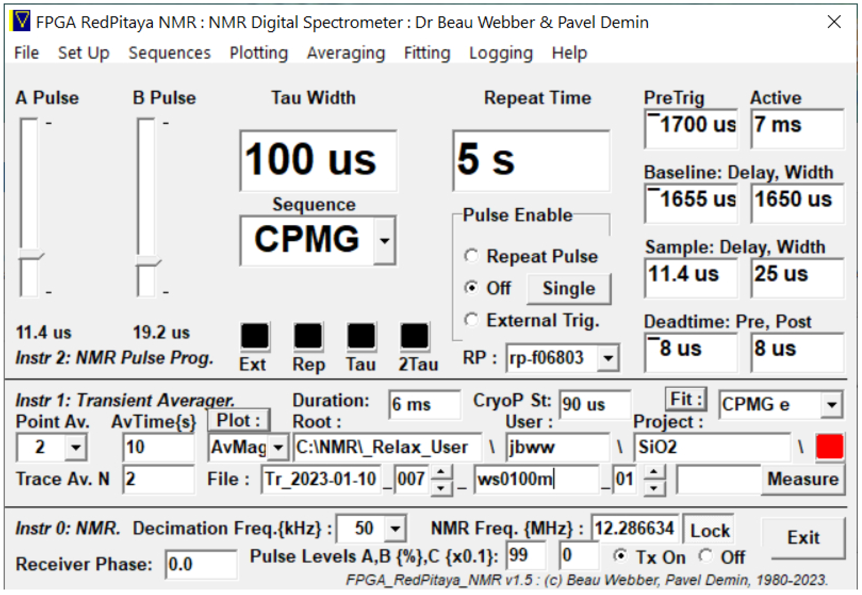
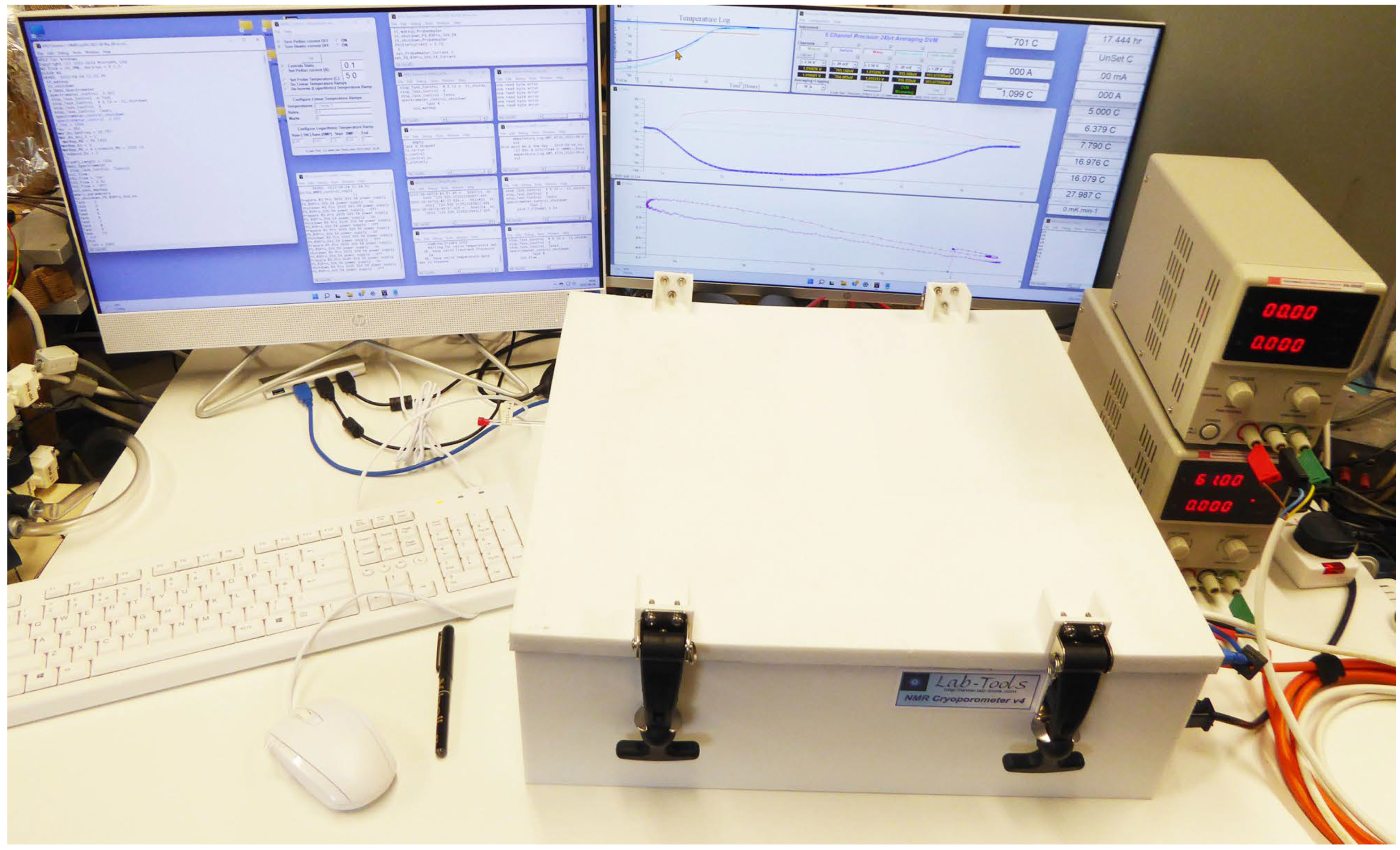
5.4. Use and Control of the Lab-Tools Mk3 NMR Spectrometer
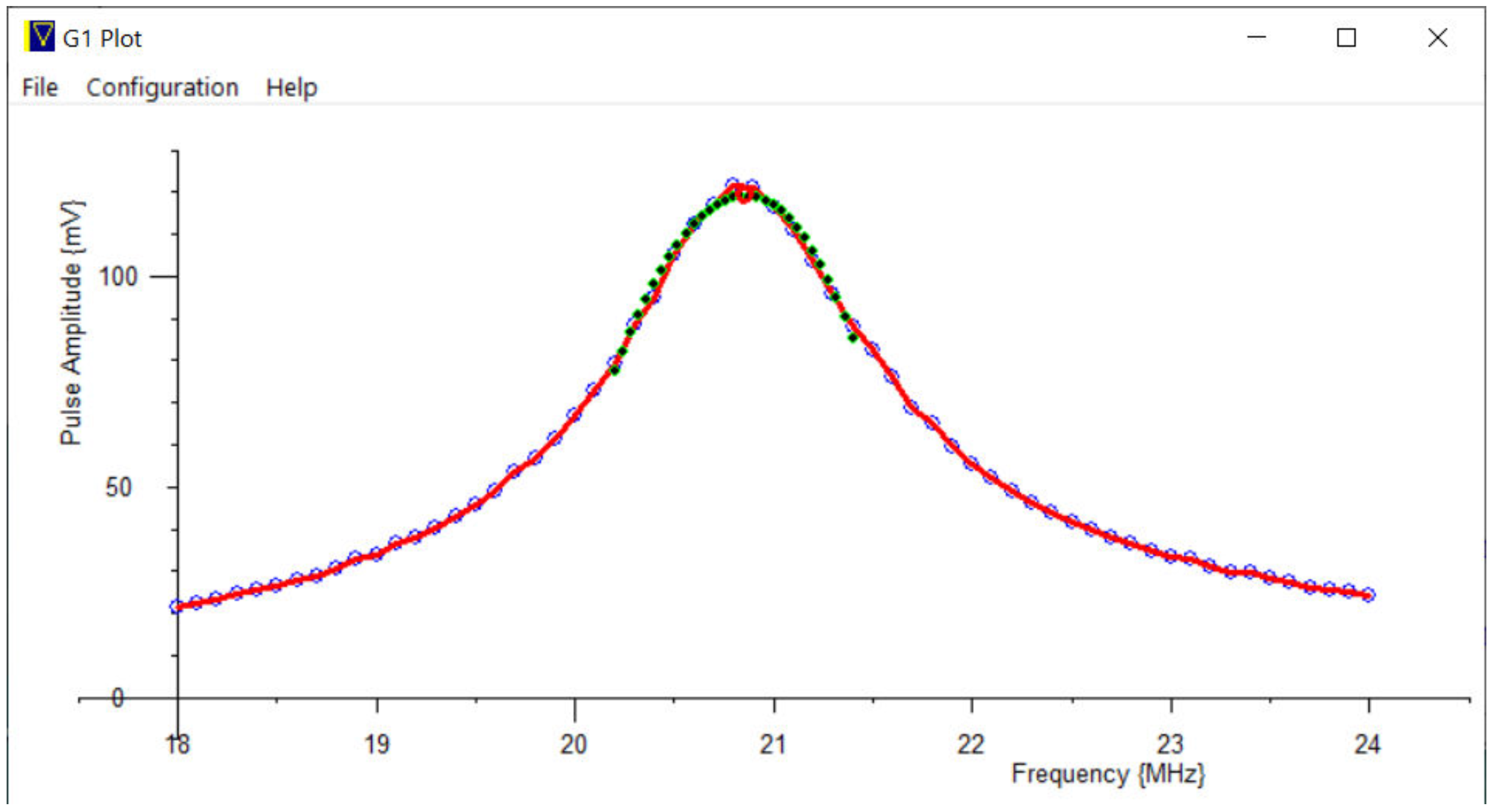
6. Setting up the Spectrometer
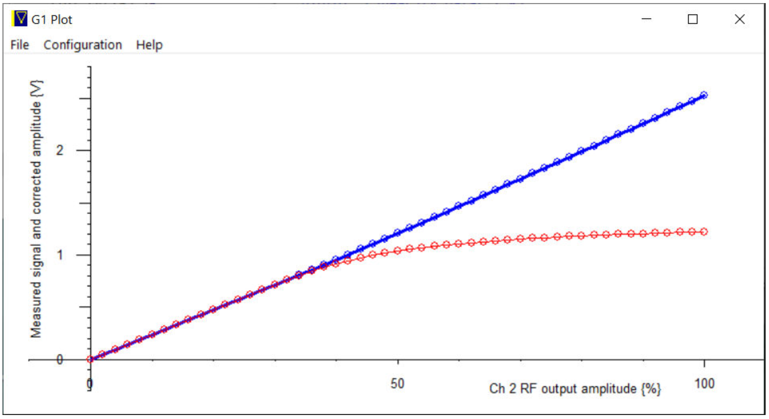
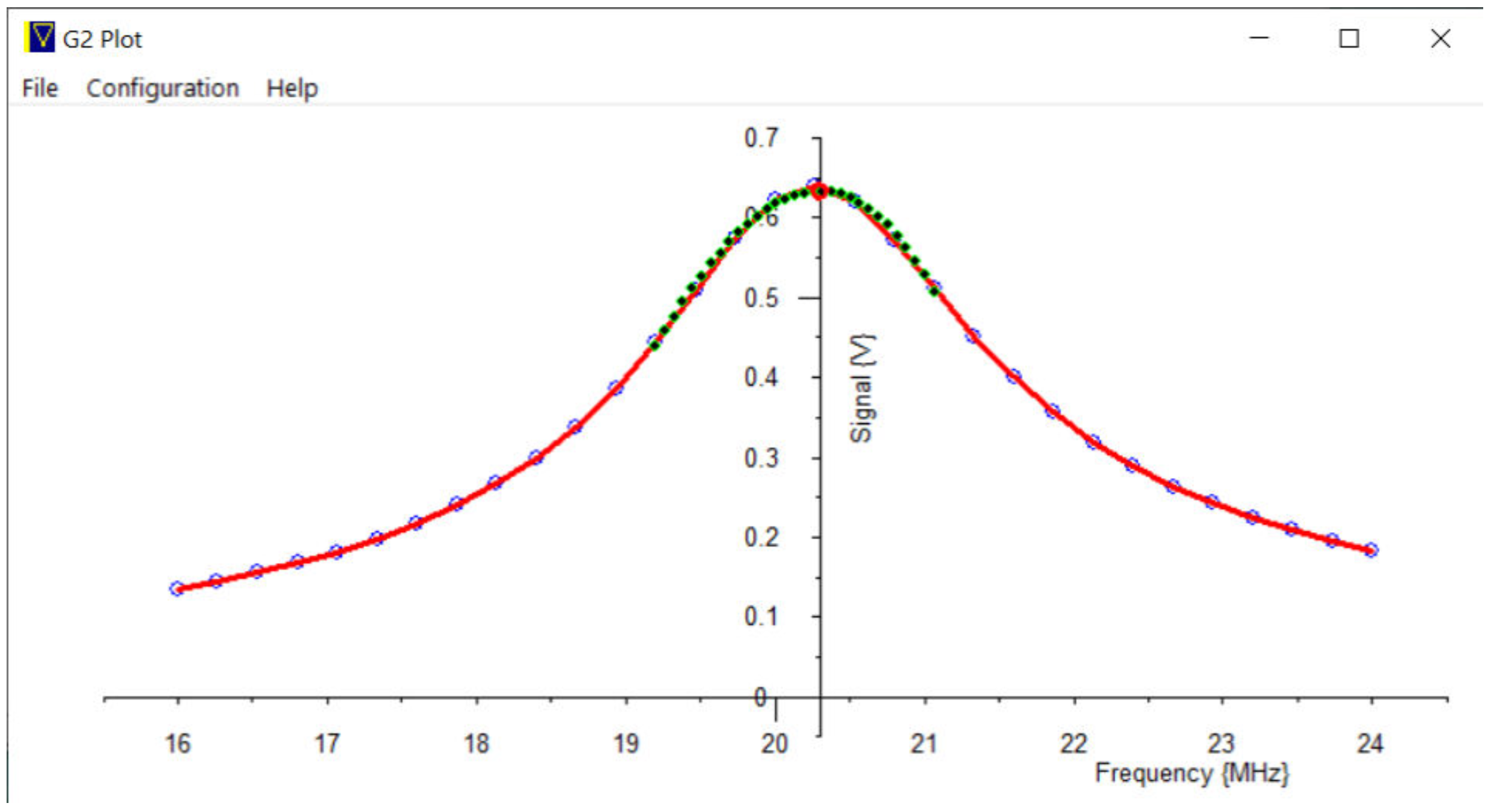
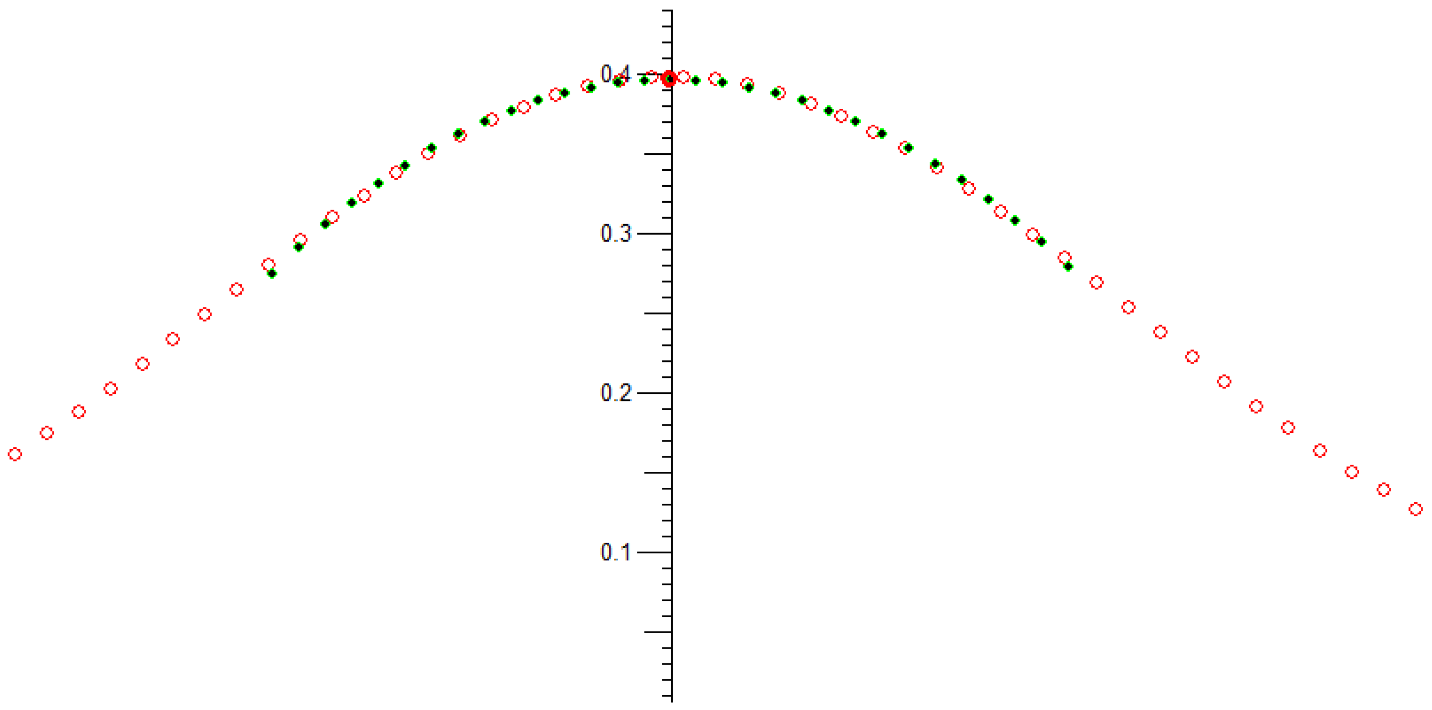
Acquiring First Signal and Auto-Tuning
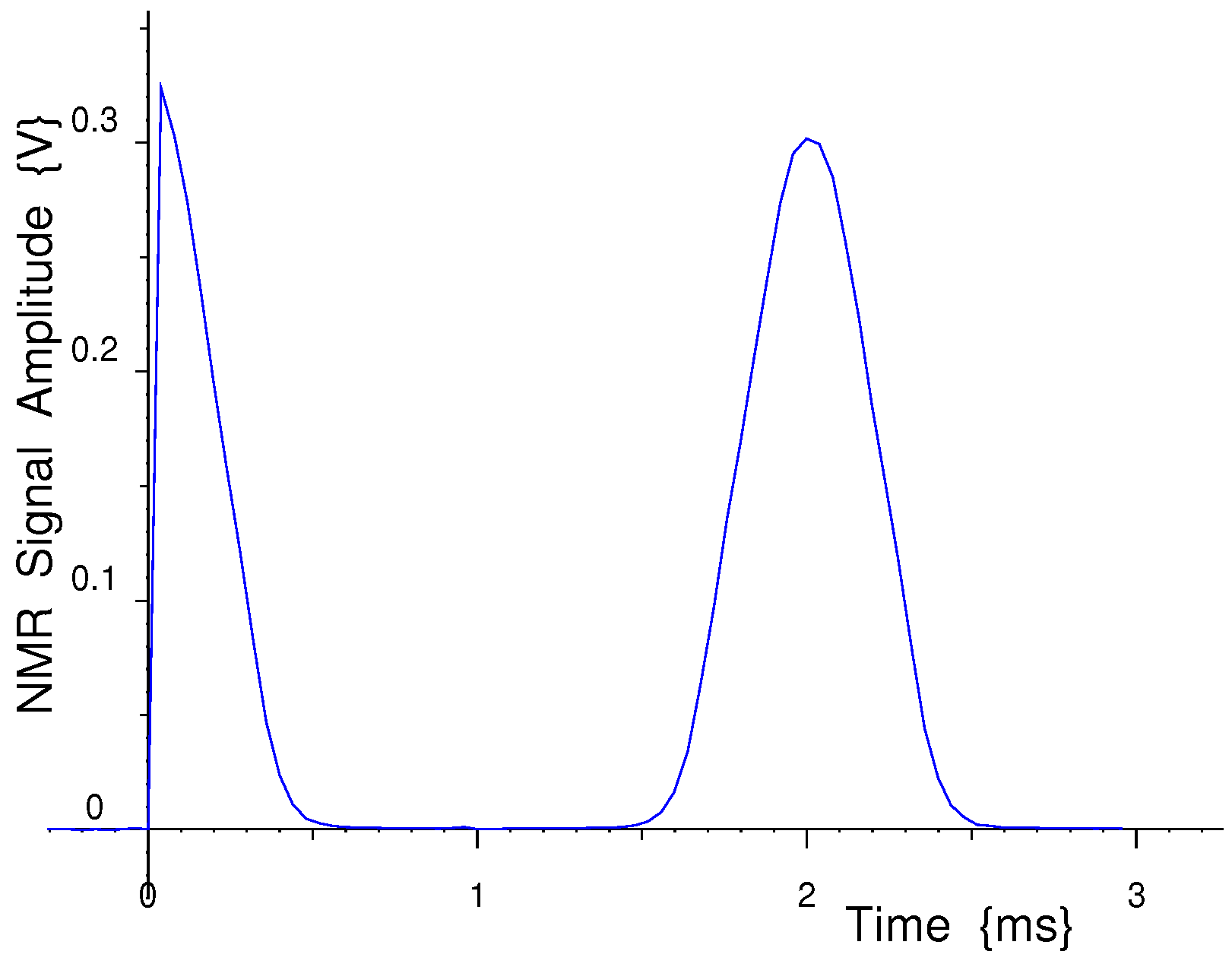
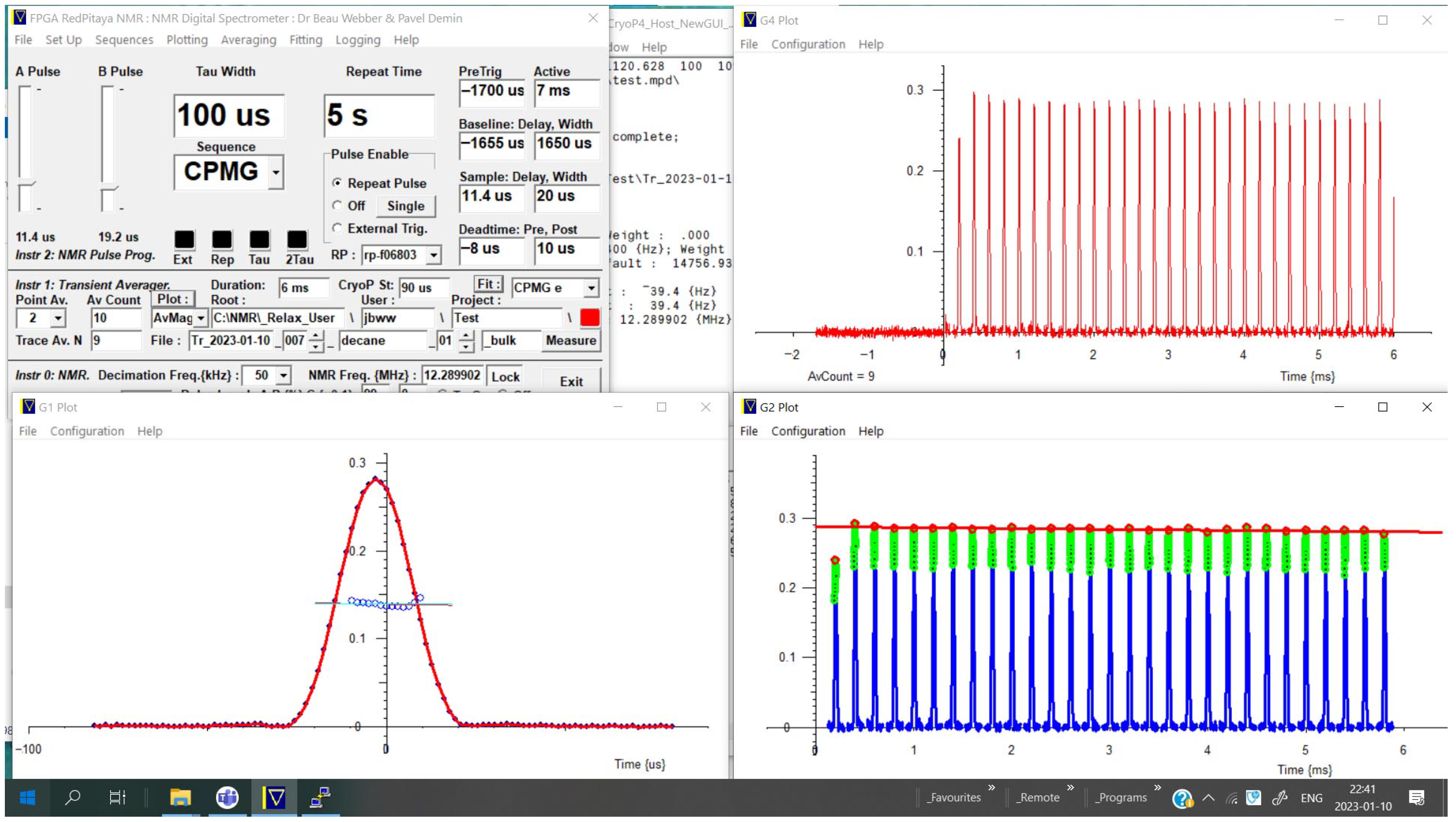
7. NMR Signal Capture, Plotting, Averaging and Online Fitting—NMR Relaxation Examples
7.1. Plotting
7.2. Averaging
7.3. Fitting
7.3.1. Single-Component Fitting
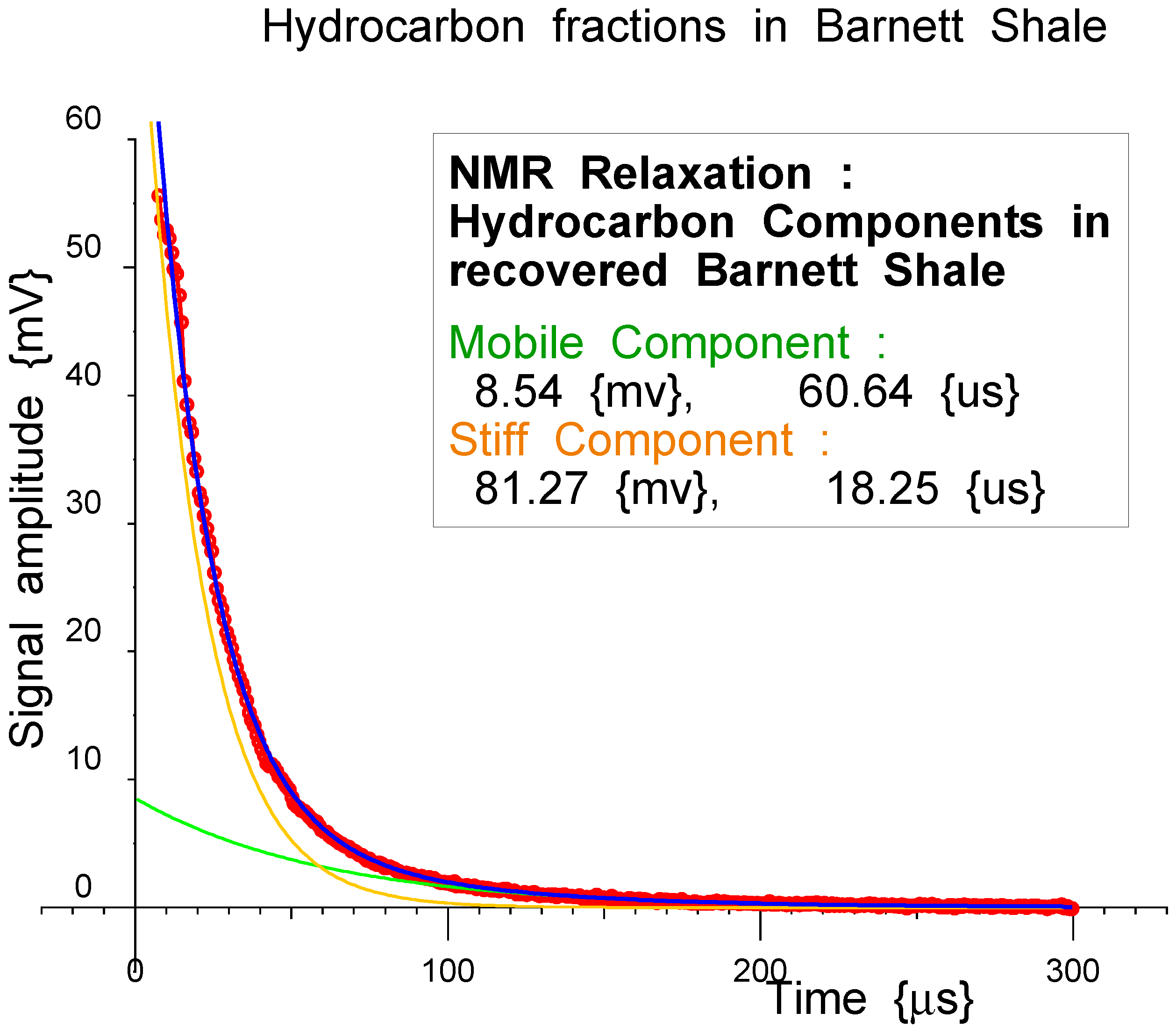
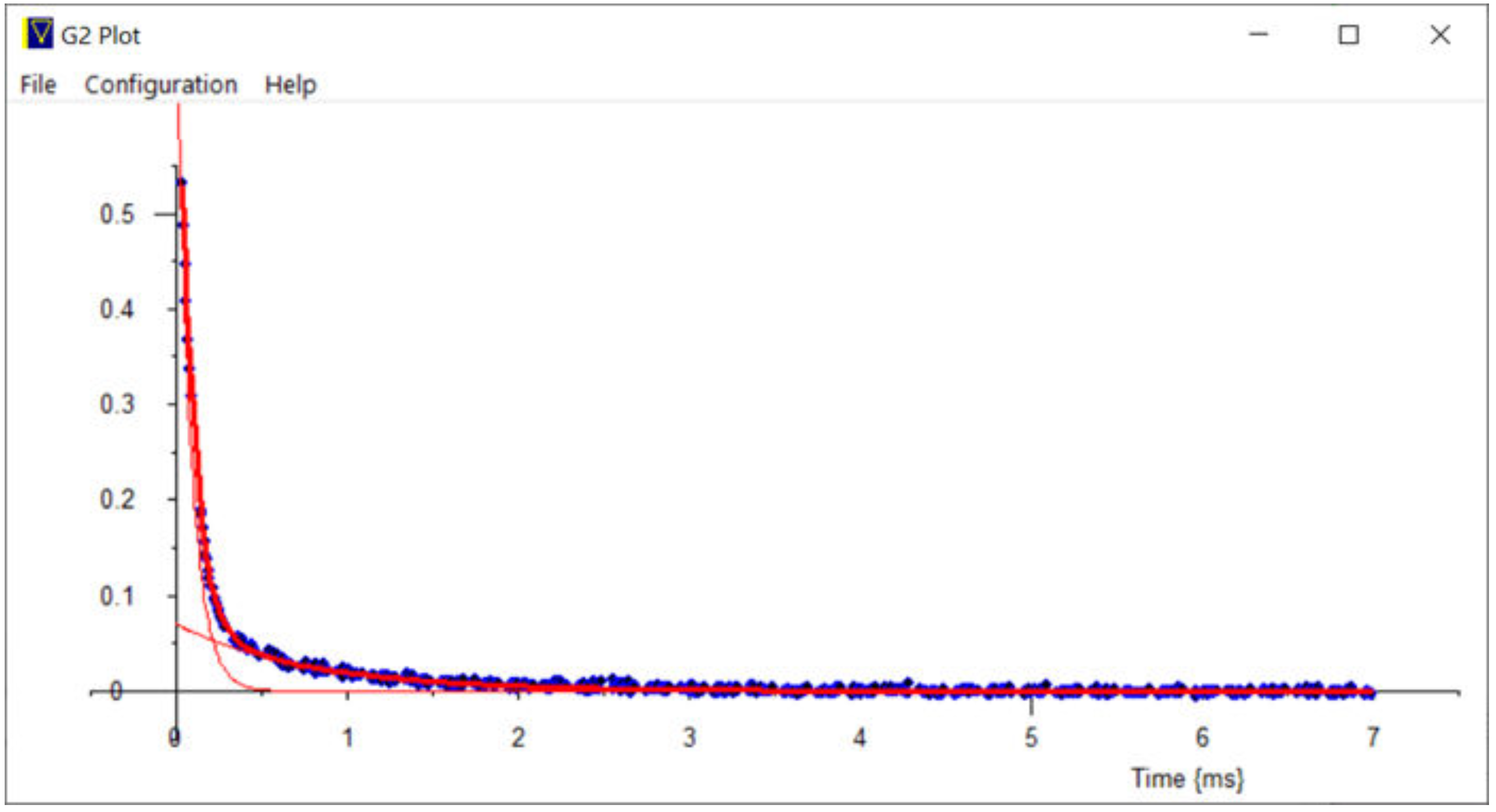
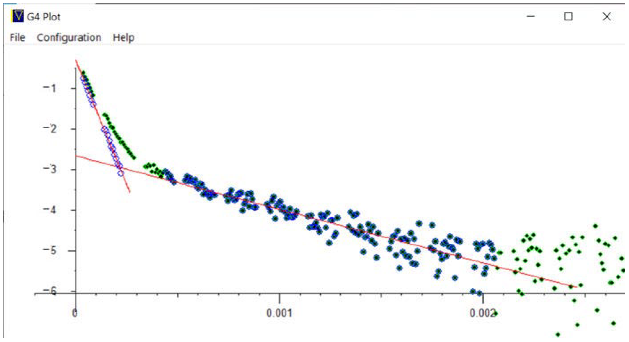
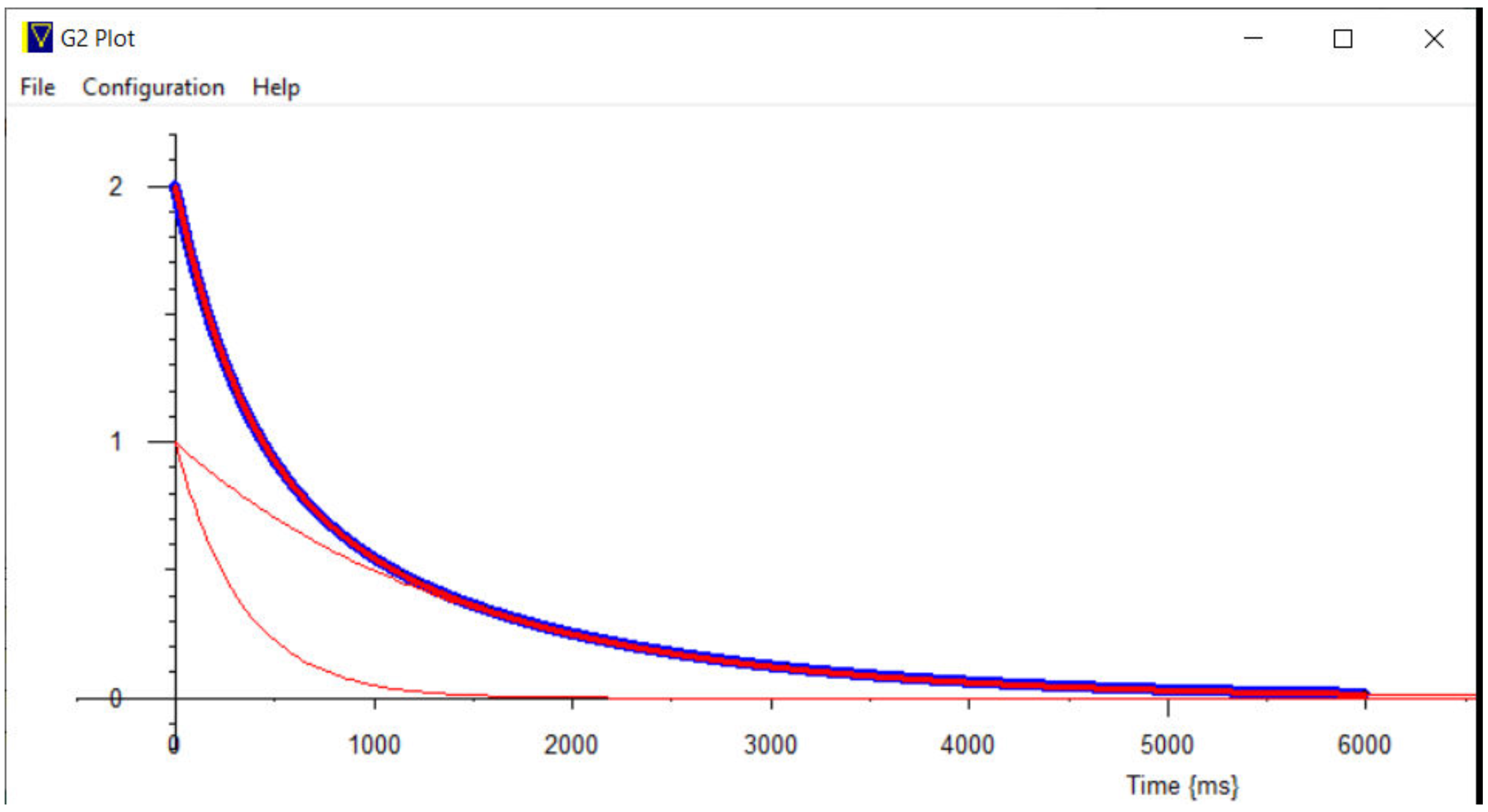
7.3.2. Two-Component Fitting
7.3.3. Fitting Echoes
7.3.4. Fitting Echo Chains
8. Variable-Temperature NMR Probe, Temperature Measurement and Control
8.1. Peltier-Cooled Variable-Temperature NMR Probe
- Referenced to a cell of distilled water maintained half frozen (Omega IceCell Model TRCIII), with a third thermocouple attached to a thermal mass in a Dewar provided a short-term temperature reference to help reduce the effect of the temperature cycling in the IceCell.
- Electronic diode junction 0 °C references have improved greatly in recent years, and these are in current use. They have the advantage of no temperature cycling.
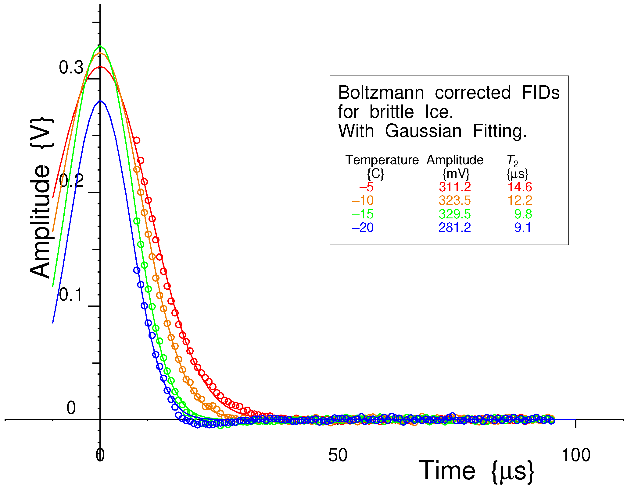
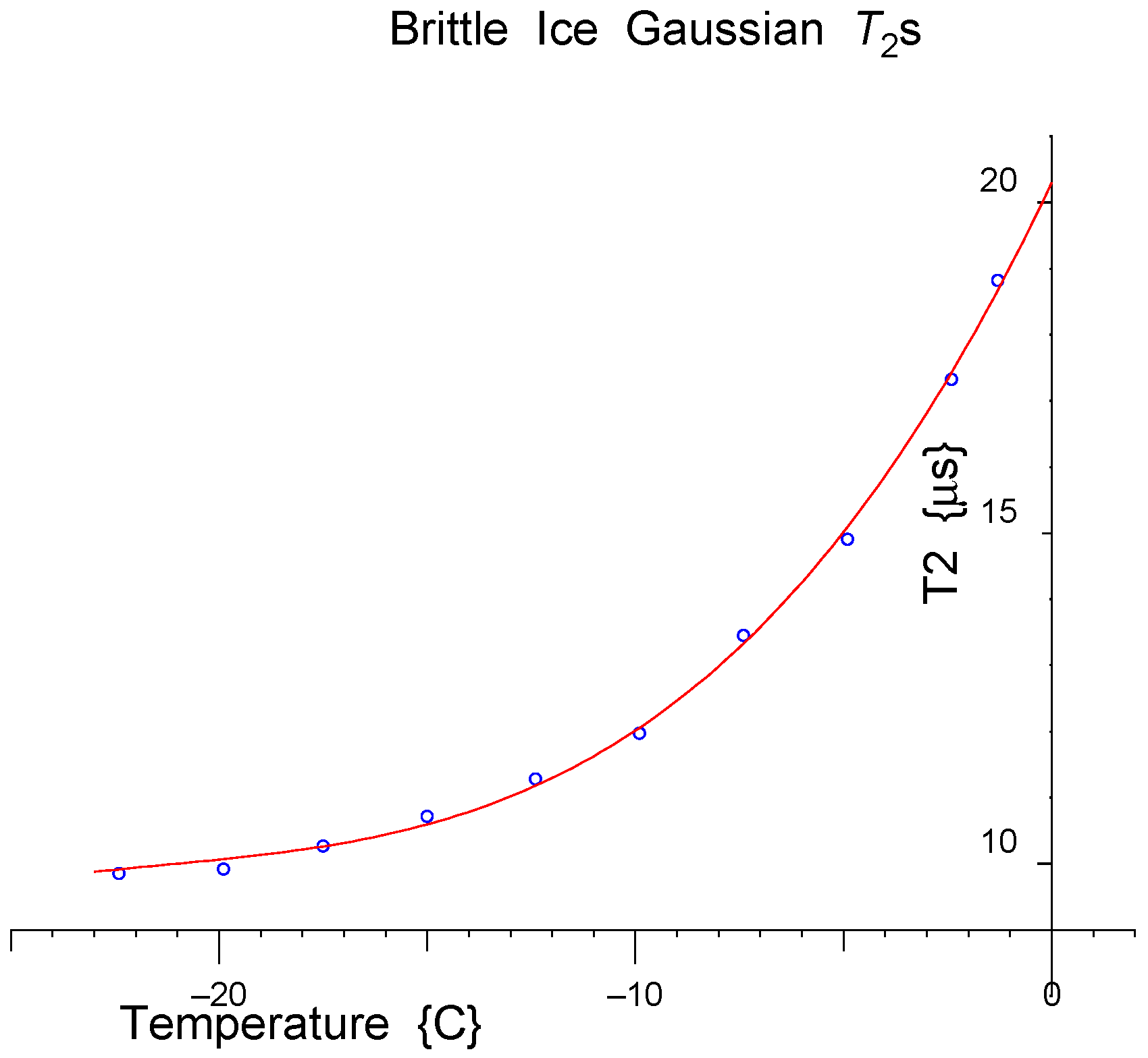
8.2. Example Variable-Temperature Measurement: Bulk Ice T2
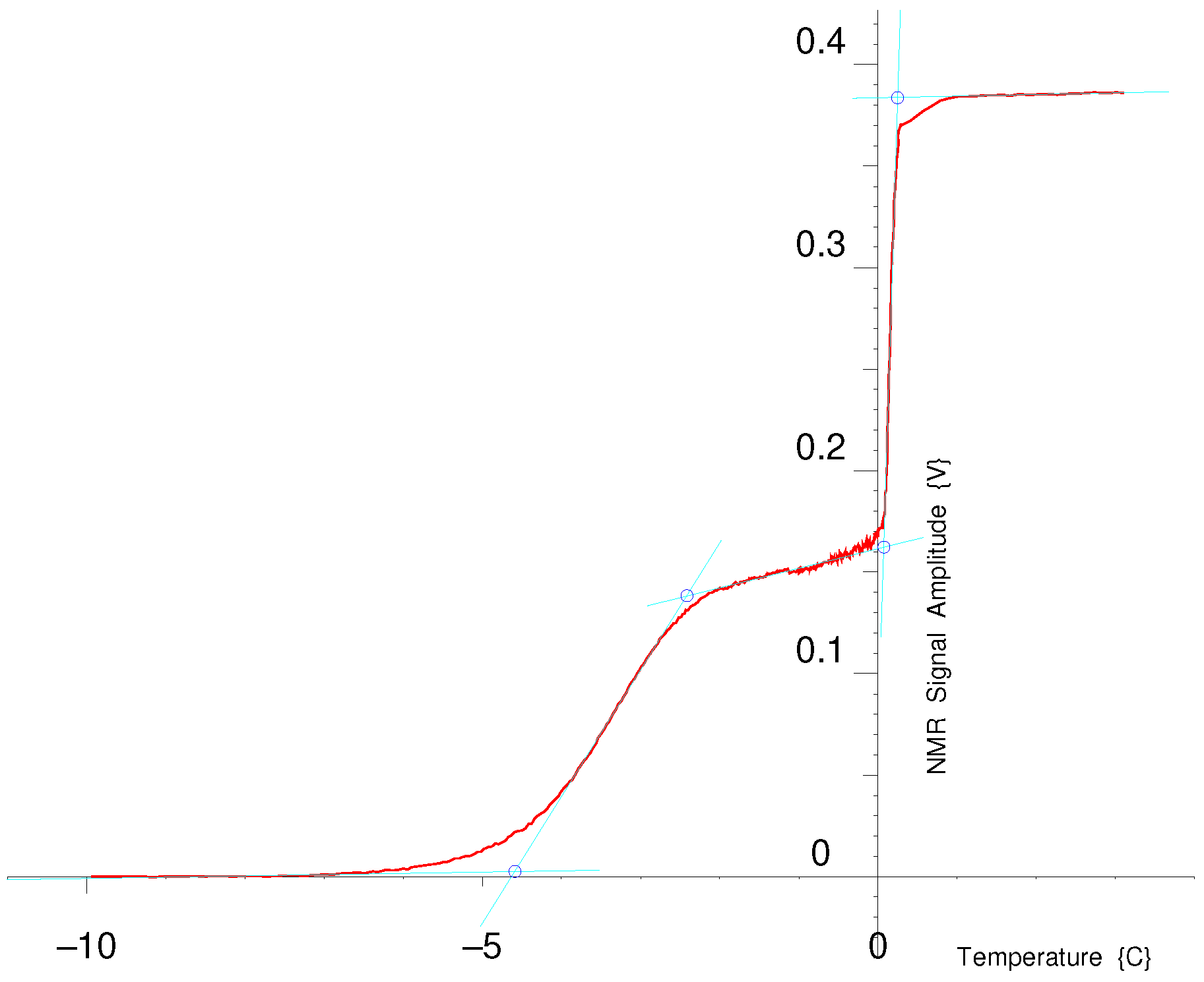
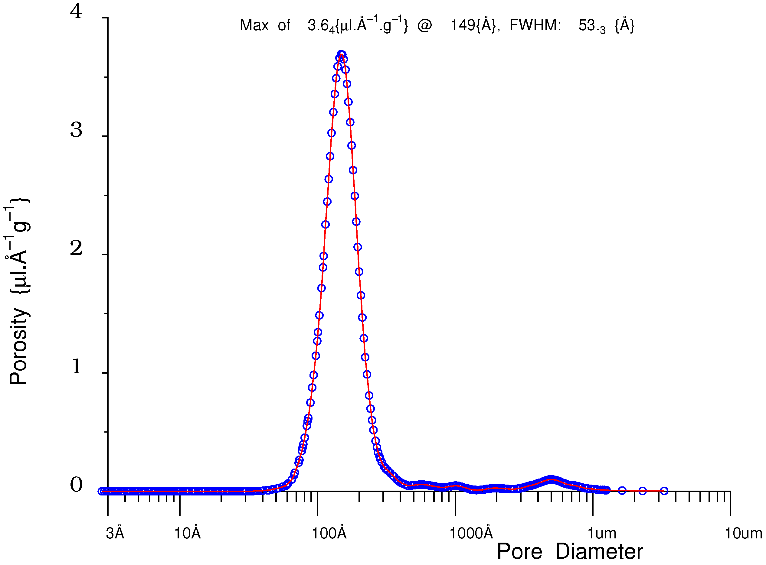
8.3. Example NMR Cryoporometric Measurement and Its Thermal Stability
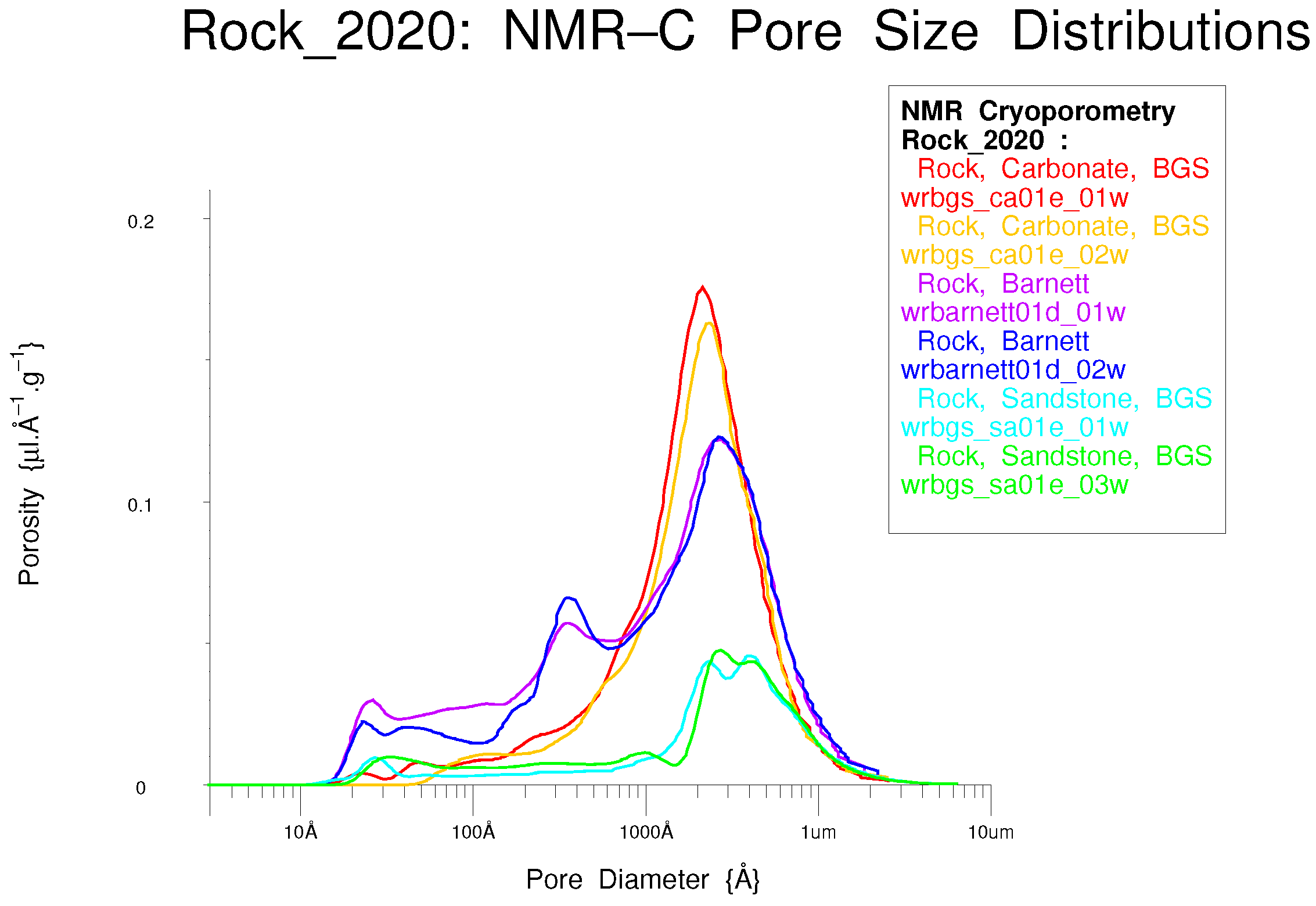
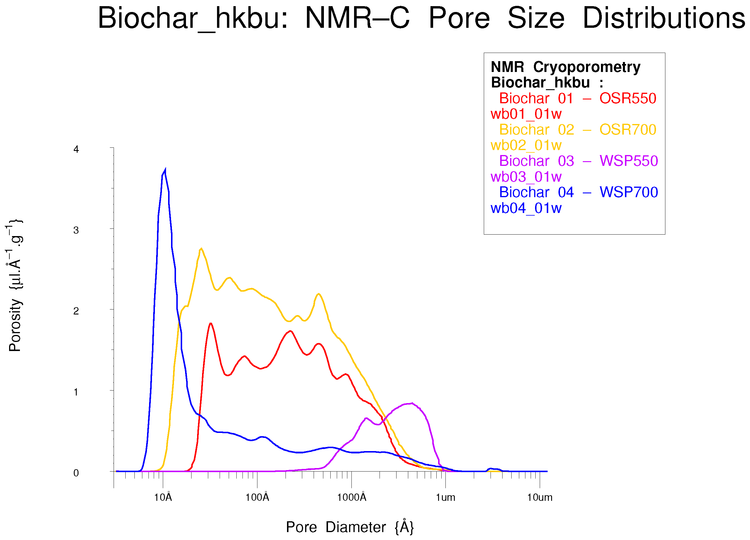
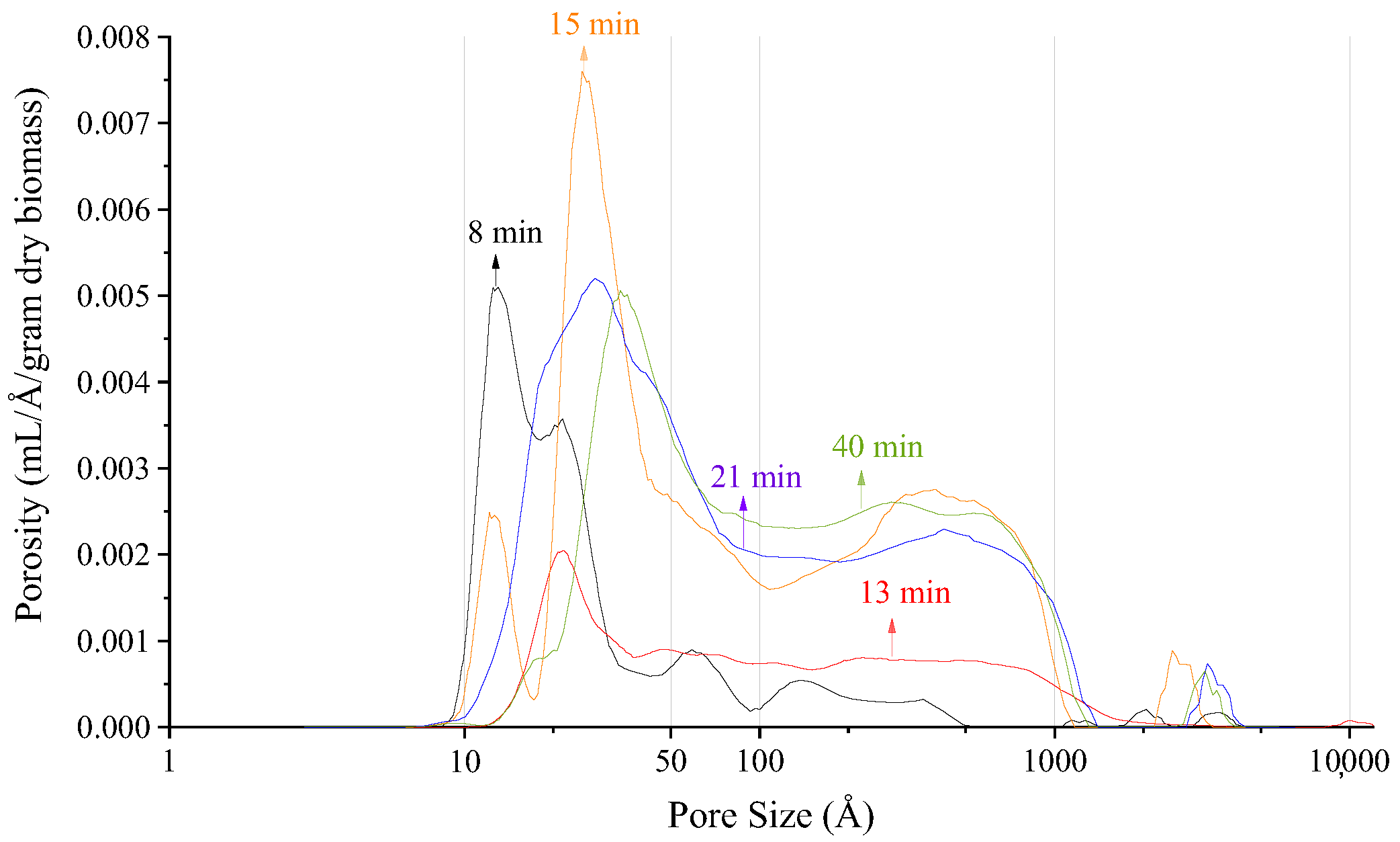
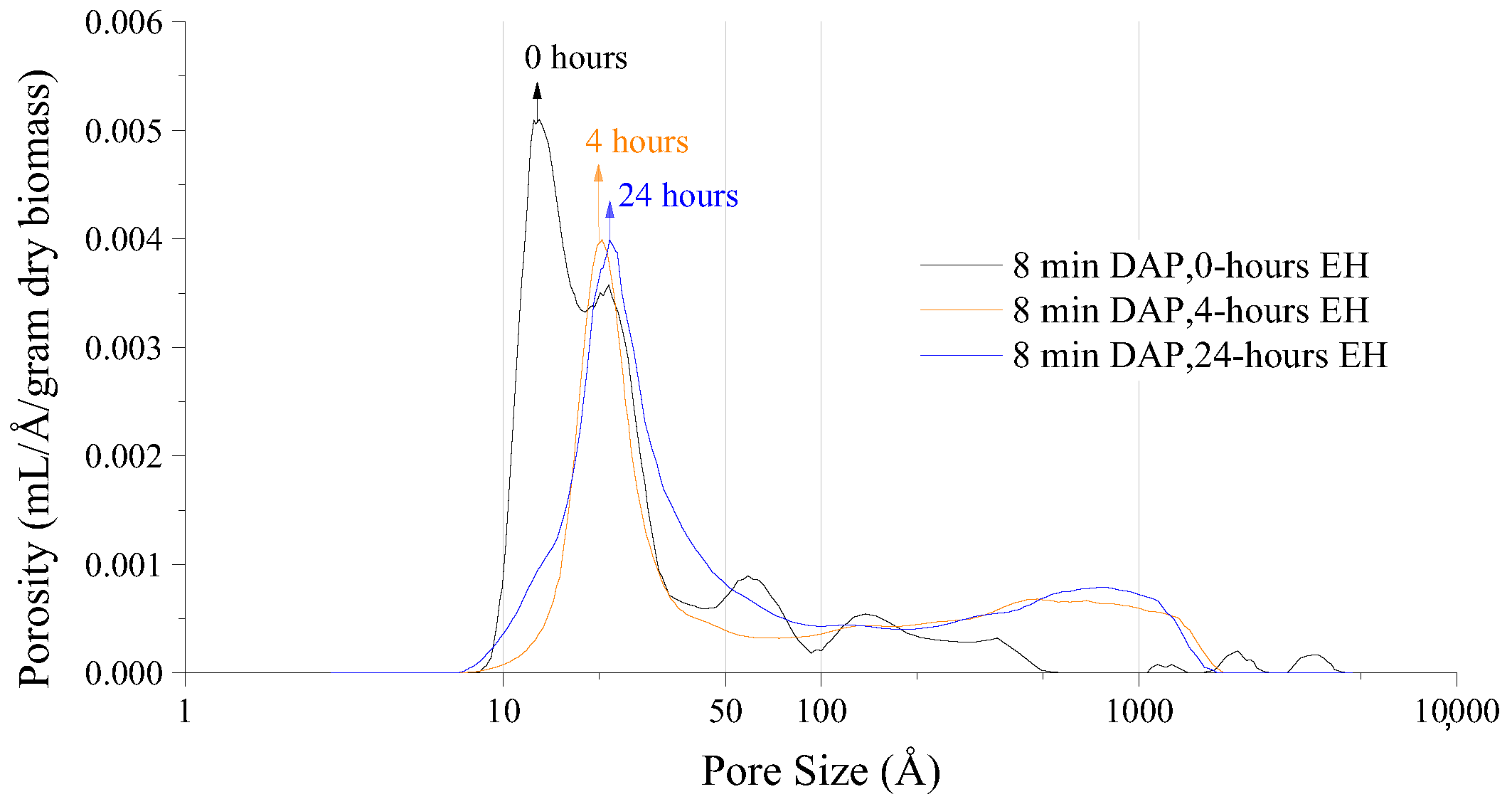
9. NMR Cryoporometric Applications
10. Further Example Applications
10.1. Measurement of 1D Imaging in a Structured Rubber Sample
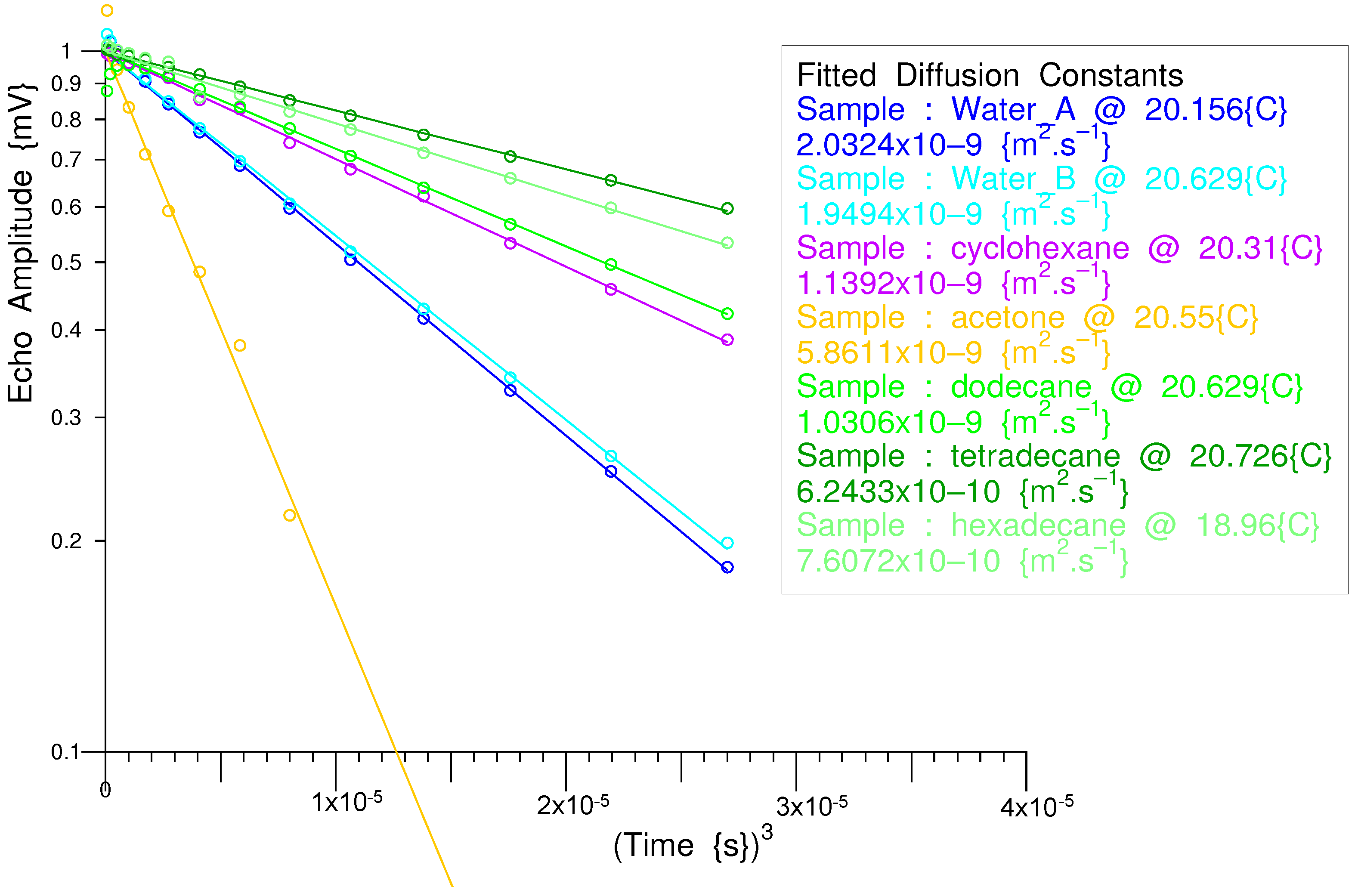
10.2. Measurement of Diffusion in Various Liquids in a 1D Magnetic Gradient
11. System Performance
System Comparisons
- (1)
- Comparison of NMR time-domain relaxation spectrometers, of which there are numerous examples. For a point-by-point comparison of 12 such instruments, including this Lab-Tools Mk3 instrument, please see Figures 5 and 6 in reference [59].
- (2)
- Comparison of NMR Cryoporometers. We know of no other commercial NMR Cryoporometers with which to make comparisons. Many commercial NMR Spectrometers may be used to make variable temperature measurements, but in most cases, the temperature control accuracy is worse by a factor of 10 or so than this dedicated NMR Cryoporometer, which limits the upper pore size that may be measured by a corresponding factor of 10.
12. Conclusions
Author Contributions
Funding
Institutional Review Board Statement
Informed Consent Statement
Data Availability Statement
Conflicts of Interest
References
- Abragam, A. The Principles of Nuclear Magnetism; Clarendon Press: Oxford, UK, 1961. [Google Scholar]
- Denise Besghini, M.M.; Simonutti, R. Time Domain NMR in Polymer Science: From the Laboratory to the Industry. Appl. Sci. 2019, 9, 1801. [Google Scholar] [CrossRef] [Green Version]
- Fabian Vaca Chavez, K.S. Time-Domain NMR Observation of Entangled Polymer Dynamics: Universal Behavior of Flexible Homopolymers and Applicability of the Tube Model. Macromolecules 2011, 44, 1549–1559. [Google Scholar] [CrossRef]
- Todt, H.; Guthausen, G.; Burk, W.; Schmalbein, D.; Kamlowski, A. Water/moisture and fat analysis by time-domain NMR. Food Chem. 2006, 96, 436–440. [Google Scholar] [CrossRef]
- Brownstein, K.; Tarr, C. Importance of classical diffusion in NMR studies of water in biological cells. Phys. Rev. A 1979, 19, 2446–2453. [Google Scholar] [CrossRef]
- Gladden, L. Nuclear-Magnetic-Resonance Studies of Porous-Media. Chem. Eng. Res. Des. 1993, 71, 657–674. [Google Scholar]
- Callaghan, P.; Godefroy, S.; Ryland, B. Diffusion-relaxation correlation in simple pore structures. J. Magn. Reson. 2003, 162, 320–327. [Google Scholar] [CrossRef]
- Fantazzini, P.; Brown, R.; Borgia, G. Bone tissue and porous media: Common features and differences studied by NMR relaxation. Magn. Reson. Imaging 2003, 21, 227–234. [Google Scholar] [CrossRef]
- Kimmich, R.; Fatkullin, N.; Mattea, C.; Fischer, E. Polymer chain dynamics under nanoscopic confinements. Magn. Reson. Imaging 2005, 23, 191–196. [Google Scholar] [CrossRef]
- Hansen, E.; Fonnum, G.; Weng, E. Pore morphology of porous polymer particles probed by NMR relaxometry and NMR cryoporometry. J. Phys. Chem. 2005, 109, 24295–24303. [Google Scholar] [CrossRef]
- McDonald, P.J.; Mitchell, J.; Mulheron, M.; Aptaker, P.S.; Korb, J.P.; Monteilhet, L. Two-dimensional correlation relaxometry studies of cement pastes performed using a new one-sided NMR magnet. Cem. Concr. Res. 2007, 37, 303–309. [Google Scholar] [CrossRef]
- D’Agostino, C.; Mitchell, J.; Mantle, M.D.; Gladden, L.F. Interpretation of NMR Relaxation as a Tool for Characterising the Adsorption Strength of Liquids inside Porous Materials. Chemistry 2014, 20, 13009–13015. [Google Scholar] [CrossRef] [Green Version]
- Webber, J.B.W. Biological, Medical and Nano Structured materials–NMR done Simply. Arch. Biomed. Eng. Biotechnol. 2019, 1. [Google Scholar] [CrossRef] [Green Version]
- Strange, J.; Mitchell, J.; Webber, J. Pore surface exploration by NMR. Magn. Reson. Imaging 2003, 21, 221–226. [Google Scholar] [CrossRef] [Green Version]
- Mitchell, J.; Webber, J.; Strange, J. Nuclear magnetic resonance cryoporometry. Phys. Rep. 2008, 461, 1–36. [Google Scholar] [CrossRef] [Green Version]
- Petrov, O.V.; Furo, I. NMR cryoporometry: Principles, applications and potential. Prog. Nucl. Magn. Reson. Spectrosc. 2009, 54, 97–122. [Google Scholar] [CrossRef]
- Rottreau, T.J.; Parkes, G.E.; Schirru, M.; Harries, J.L.; Mesa, M.G.; Topham, P.D.; Evans, R. NMR Cryoporometry of Polymers: Cross-linking, Porosity and the Importance of Probe Liquid. Colloids Surf. A Physicochem. Eng. Asp. 2019, 575, 256–263. [Google Scholar] [CrossRef]
- Webber, J.B.W. Some Applications of a Field Programmable Gate Array Based Time-Domain Spectrometer for NMR Relaxation and NMR Cryoporometry. Appl. Sci. 2020, 10, 2714. [Google Scholar] [CrossRef] [Green Version]
- Gibbs, J. Collected Works; Longmans, Green and Co.: New York, NY, USA, 1928. [Google Scholar]
- Gibbs, J. The Scientific Papers of J. Willward Gibbs; Vol. I: Thermodynamics; Dover Publications, Inc.: New York, NY, USA; Constable and Co.: London, UK, 1961. [Google Scholar]
- Gibbs, J. On the equilibrium of hetrogeneous substances. In Transactions of the Connecticut Academy of Arts and Sciences; Connecticut Academy: New Haven, CT, USA, 1876; Volume III, pp. 108–248. [Google Scholar]
- Webber, J.B.W. Lab-Tools Mk3 NMR Relaxometer, Lab-Tools (Nano-Science); Ramsgate: Kent, UK, 2019. [Google Scholar]
- Webber, J.B.W. Lab-Tools Mk3 NMR Cryoporometer, Lab-Tools (Nano-Science); Ramsgate: Kent, UK, 2019. [Google Scholar]
- Belmonte, S.B.; Sarthour, R.S.; Oliveira, I.S.; Guimaes, A.P. A field-programmable gate-array-based high-resolution pulse programmer. Meas. Sci. Technol. 2003, 14, N1. [Google Scholar] [CrossRef]
- Hemnani, P.; Rajarajan, A.; Joshi, G.; Ravindranath, S. FPGA Based RF Pulse Generator for NQR/NMR Spectrometer. Procedia Comput. Sci. 2016, 93, 161–168. [Google Scholar] [CrossRef] [Green Version]
- Takeda, K. A highly integrated FPGA-based nuclear magnetic resonance spectrometer. Rev. Sci. Instrum. 2007, 78, 033103. [Google Scholar] [CrossRef]
- Webber, J.B.W.; Corbett, P.; Semple, K.T.; Ogbonnaya, U.; Teel, W.S.; Masiello, C.A.; Fisher, Q.J.; Valenza, J.J., II; Song, Y.-Q.; Hu, Q. An NMR study of porous rock and biochar containing organic material. Microporous Mesoporous Mater. 2013, 178, 94–98. [Google Scholar] [CrossRef]
- Webber, J.B.W. Nuclear Magnetic Resonance Probes. U.S. Patent 9,810,750 B2, 7 November 2017. [Google Scholar]
- Webber, J.; Strange, J.; Dore, J. An evaluation of NMR cryoporometry, density measurement and neutron scattering methods of pore characterisation. Magn. Reson. Imaging 2001, 19, 395–399. [Google Scholar] [CrossRef] [PubMed] [Green Version]
- Webber, J.B.W. Accessible Catalyst Pore Volumes, for Water and Organic Liquids, as probed by NMR Cryoporometry. Diffusion-fundamentals.org 2014, 22, 1–8. [Google Scholar]
- Andrey, A.S.; Beau Webber, P.S. Advanced NMR for Industrial Applications: Structure, Porosity, and Acidity; Characterization of Catalytic Materials through a Facile Approach to Probe OH Groups; Total Research and Technology Feluy (TRTF); Lab-Tools Ltd.: Ramsgate, UK, 2019. [Google Scholar]
- Webber, J.B.W.; Livadaris, V.; Andreev, A.S. USY zeolite mesoporosity probed by NMR cryoporometry. Microporous Mesoporous Mater. 2020, 306, 110404. [Google Scholar] [CrossRef]
- Workman, M.J.; Webber, J.B.W.; Perry, M.L.; Darling, R.M.; More, K.L.; Mukundan, R.; Borup, R.L. Analysis of PEMFC Electrode Structure–Bridging the Mesoscale Gap. In Proceedings of the 236th Meeting of the Electrochemical Society, Atlanta, GA, USA, 13–17 October 2019. [Google Scholar]
- Boguszynska, J.; Tritt-Goc, J. H-1 NMR cryoporometry study of the melting behavior of water in white cement. Z. Naturforschung Sect. A-J. Phys. Sci. 2004, 59, 550–558. [Google Scholar] [CrossRef]
- Fleury, M.; Fabre, R.; Webber, J.W. Comparison of Pore Size Distribution by NMR Relaxation and NMR Cryoporometry in Shales. In Proceedings of the International Symposium of the Society of Core Analysts, St. John’s, NL, Canada, 16–21 August 2015; 12p. [Google Scholar]
- Ankathi, S.K.; Zhou, W.; Webber, J.B.; Patil, R.; Chaudhari, U.; Shonnard, D. Synergistic Effects between Hydrolysis Time and Microporous Structure in Poplar. ACS Sustain. Chem. Eng. 2019, 7, 12920–12929. [Google Scholar] [CrossRef]
- Aditya Rawal, S.D.J.; Webber, J.B.W. Mineral-Biochar Composites: Molecular Structure and Porosity. Environ. Sci. Technol. 2016, 50, 7706–7714. [Google Scholar] [CrossRef] [Green Version]
- Wong, J.; Webber, J.; Ogbonnaya, U. Characteristics of biochar porosity by NMR and study of ammonium ion adsorption. J. Anal. Appl. Pyrolysis 2019, 143, 104687. [Google Scholar] [CrossRef]
- Strange, J.; Webber, J. Characterization of Porous Solids by NMR. In Proceedings of the 12th Specialized Colloque Ampere, Corfu, Greece, 10–15 September 1995. [Google Scholar]
- Red Pitaya FPGA Module. Available online: https://redpitaya.com/red-pitaya-in-research/ (accessed on 29 March 2023).
- Webber, J.B.W.; Demin, P. Credit-card sized field and benchtop NMR relaxometers using field programmable gate arrays. Magn. Reson. Imaging 2019, 56, 45–51. [Google Scholar] [CrossRef]
- British Standards. 2013. Online Resource. Available online: https://www.en-standard.eu/une-en-61326-1-2013-electrical-equipment-for-measurement-control-and-laboratory-use-emc-requirements-part-1-general-requirements-endorsed-by-aenor-in-march-of-2013/ (accessed on 24 March 2023).
- IEC Standards. 2012. Online Resource. Available online: https://www.document-center.com/standards/show/IEC-61326-1 (accessed on 24 March 2023).
- Xilinx Partners. IP library by Xilinx. Technical Report, Xilinx.com. 2021. Online Resource. Available online: https://www.xilinx.com/products/intellectual-property.html (accessed on 29 March 2023).
- Demin, P. Pavel Demin Pulsed NMR Firmware. Technical Report. 2021. Online Resource. Available online: https://pavel-demin.github.io/red-pitaya-notes/pulsed-nmr (accessed on 29 March 2023).
- Xilinx Partners. Xilinx–Direct Digital Synthesizer (DDS). Technical Report, Xilinx.com. 2021. Online Resource. Available online: https://docs.xilinx.com/v/u/en-US/pg141-dds-compiler (accessed on 29 March 2023).
- Xilinx Partners. Xilinx–Macro for Abstraction of the DSP48 Slice Module. Technical Report, Xilinx.com. 2020. Online Resource. Available online: https://docs.xilinx.com/r/en-US/pg323-dsp-macro (accessed on 29 March 2023).
- Xilinx Partners. Xilinx–Cascaded Integrator Comb (CIC) Filter Compiler. Technical report, Xilinx.com. 2016. Online Resource. Available online: https://docs.xilinx.com/v/u/en-US/pg140-cic-compiler (accessed on 29 March 2023).
- Xilinx Partners. Xilinx–Finite Impulse Response (FIR) Filter Compiler. Technical report, Xilinx.com. 2021. Online Resource. Available online: https://docs.xilinx.com/r/en-US/pg149-fir-compiler (accessed on 29 March 2023).
- Iverson, K. A Programming Language; Wiley: New York, NY, USA, 1962. [Google Scholar]
- Demin, P. Source Code for the Pulsed NMR TCP Server. Technical Report. 2020. Online Resource. Available online: https://github.com/pavel-demin/red-pitaya-notes/blob/master/projects/pulsed_nmr/server/pulsed-nmr.c (accessed on 29 March 2023).
- Demin, P. Source Code for the Pulsed NMR TCP client .NET Library. Technical report. 2020. Online Resource. Available online: https://github.com/pavel-demin/red-pitaya-notes/blob/master/projects/pulsed_nmr/client/PulsedNMR.cs (accessed on 29 March 2023).
- Norris, M.O.; Strange, J.H. A nuclear magnetic resonance sample temperature controller using liquid nitrogen injection. J. Phys. E Sci. Instrum. 1969, 2, 1106–1108. [Google Scholar] [CrossRef]
- Wikipedia. Dry Ice–Is the Solid Form of Carbon Dioxide. Technical report, Wikipedia. 2019. Online Resource. Available online: https://en.wikipedia.org/wiki/Dry_ice (accessed on 26 March 2023).
- Meyer, C.W.; Garrity, K.M. Updated uncertainty budgets for NIST thermocouple calibrations. In Proceedings of the AIP Conference Proceedings, Physical Measurement Laboratory/Sensor Science Division, Thermodynamic Metrology Group, Los Angeles, CA, USA, 19–23 March 2013; p. 1552. [Google Scholar] [CrossRef] [Green Version]
- Webber, J.B.W. The Characterisation of Porous Media. Ph.D. Thesis, Physics. University of Kent, Canterbury, UK, 2000. [Google Scholar]
- Biochar Systems Using Biomass as an Energy Source for Developing Countries. Summary from World Bank: “Biochar Systems for Smallholders in Developing Countries. 2015. Online Resource. Available online: https://documents.worldbank.org/en/publication/documents-reports/documentdetail/188461468048530729/biochar-systems-for-smallholders-in-developing-countries-leveraging-current-knowledge-and-exploring-future-potential-for-climate-smart-agriculture (accessed on 24 March 2023).
- Torrey, H.C. Bloch Equations with Diffusion Terms. Phys. Rev. 1956, 104, 563. [Google Scholar] [CrossRef]
- Webber, J.B.W. A review of the use of simple time-domain NMR/MRI for material-science. SN Appl. Sci. 2021, 3, 809. [Google Scholar] [CrossRef]


| A |
| B |
| AA |
| AB |
| BA |
| EqGhain |
| CPMG |
| T1Rho |
Disclaimer/Publisher’s Note: The statements, opinions and data contained in all publications are solely those of the individual author(s) and contributor(s) and not of MDPI and/or the editor(s). MDPI and/or the editor(s) disclaim responsibility for any injury to people or property resulting from any ideas, methods, instructions or products referred to in the content. |
© 2023 by the authors. Licensee MDPI, Basel, Switzerland. This article is an open access article distributed under the terms and conditions of the Creative Commons Attribution (CC BY) license (https://creativecommons.org/licenses/by/4.0/).
Share and Cite
Webber, J.B.W.; Demin, P. Digitally Based Precision Time-Domain Spectrometer for NMR Relaxation and NMR Cryoporometry. Micro 2023, 3, 404-433. https://doi.org/10.3390/micro3020028
Webber JBW, Demin P. Digitally Based Precision Time-Domain Spectrometer for NMR Relaxation and NMR Cryoporometry. Micro. 2023; 3(2):404-433. https://doi.org/10.3390/micro3020028
Chicago/Turabian StyleWebber, John Beausire Wyatt, and Pavel Demin. 2023. "Digitally Based Precision Time-Domain Spectrometer for NMR Relaxation and NMR Cryoporometry" Micro 3, no. 2: 404-433. https://doi.org/10.3390/micro3020028