Article

Solvent and H/D Isotopic Substitution Effects on the Krichevskii Parameter of Solutes: A Novel Approach to Their Accurate Determination

by
Ariel A. Chialvo
1,* and
Oscar D. Crisalle
2
1
Independent Researcher, Knoxville, TN 37922-3108, USA
2
Department of Chemical Engineering, University of Florida, Gainesville, FL 32611-6005, USA
*
Author to whom correspondence should be addressed.
Liquids 2022, 2(4), 474-503; https://doi.org/10.3390/liquids2040028
Submission received: 11 November 2022 / Revised: 7 December 2022 / Accepted: 8 December 2022 / Published: 15 December 2022
(This article belongs to the Section Chemical Physics of Liquids)

Abstract

:
We establish a direct route for the accurate determination of the solvent effect on the Krichevskii parameter of a solute, based solely on the contrasting solvation behavior of the solute in the desired solvent relative to that of the reference solvent, i.e., in terms of the distinct solvation Gibbs free energies of the solute and the corresponding Krichevskii parameters of an ideal gas solute in the pair of solvents. First, we illustrate the proposed approach in the determination of the H / D solvent effect on the Krichevskii parameter of gaseous solutes in aqueous solutions, when the solvents are different isotopic forms (isotopomers) of water, and then, by generalizing the approach to any pair of solvents. For that purpose, we (a) identify the links between the standard solvation Gibbs free energy of the i solute in the two involved solvent environments and the resulting Krichevskii parameters, (b) discuss the fundamentally based linear behavior between the Krichevskii parameter and the standard solvation Gibbs free energy of the i solute in an α solvent, and interpret two emblematic cases of solutions involving either an ideal gas solute or an i solute behaving identically as the solvating species, as well as (c) provide a novel microstructural interpretation of the solvent effect on the Krichevskii parameter according to a rigorous characterization of the critical solvation as described by a finite unambiguous structure making/breaking parameter S i α ( S R ) of the i solute in the pair of α solvents.

Graphical Abstract

1. Introduction

The Krichevskii parameter defines a finite-size quantity as the limiting critical value of the isothermal-isochoric rate of change of the system’s pressure caused by the mutation (aka alchemical transformation) of an α solvent particle into an i solute species, in an otherwise pure solvent, i.e., lim T , ρ α o c r i t i c a l ( P / x i ) T ρ A K r [1]. Even though A K r is a finite quantity, its magnitude and sign are the result of the underlying solute-solvent intermolecular interaction asymmetry [2,3,4], where the developing pressure perturbation propagates across the entire system given that the solvent’s correlation length diverges at criticality [5,6].
The interest on the Krichevskii parameter has grown immensely since its inception [2], in part, because it has become a key quantity in the description and/or correlation of the thermodynamic behavior of dilute solutions, especially for non-electrolyte aqueous systems [7,8,9,10,11,12,13]. Its relevance has generated the urgency for experimental approaches to its determination, involving a variety of methodologies as discussed elsewhere [14,15,16]. Unfortunately, the accumulated tabulations of Krichevskii parameters, especially involving light and heavy water as well as carbon dioxide as solvents [15,16,17,18,19,20,21], involve significantly large uncertainties [4,14,22], a condition that hinders our ability to make accurate interpretations [23].
On the one hand, this (uncertainty) issue becomes exacerbated when studying the solvation of gases in isotopomers of a solvent such as light and heavy water, where the isotopic effect on the Krichevskii parameters given by their “brute-force” difference ( A K r i , D 2 O A K r i , H 2 O ) , is typically more than an order of magnitude smaller than the observed uncertainties of A K r i , α for the individual α isotopic form of the solvent [24]. In other words, this is the undesirable situation involving typically small differences between two large quantities exhibiting significant uncertainties whose outcome is substantially smaller than its combined uncertainty.
On the other hand, it appears appealing to have a direct route for the assessment of the effect of the type of solvent on the resulting Krichevskii parameter based solely on the contrasting solvation characteristic of the i solute in the desired k solvent, relative to that of a reference j solvent, i.e., in terms of the distinctive standard solvation Gibbs free energies of the solute and the Krichevskii parameters of an ideal gas solute in the pair of solvents. Indeed, the matter we would like to address here can be encapsulated in the following two questions: (a) how could we determine the Krichevskii parameter of an i solute in a k solvent, A K r i , k , when we accurately know not only the solvation behavior of the i solute in a j solvent at ambient conditions but also, its Krichevskii parameter A K r i , j ?, and (b) how could we determine directly the change in the Krichevskii parameter of an i solute, Δ A K r A K r i , k A K r i , j , when we replace the j solvent with a k solvent and simultaneously know accurately the solvation behavior at ambient conditions of the i solute in both solvents?
In this work, we suggest an approach to answer these questions, by establishing routes for the determination of the isotopic effect on the Krichevskii parameter of a solute, i.e., when the solvents are isotopomers, and then, by generalizing the approach to any pair of solvents. For that purpose, in Section 2, we provide the thermodynamic foundations underlying the isobaric-isothermal transfer of an i solute from the j solvent phase to the k solvent phase, as characterized by the transfer Gibbs free energy of the dilute solute. Therefore, we draw the link between the standard solvation Gibbs free energy of the i solute in the pair of solvent environments, Δ h G i , α , and the resulting Krichevskii parameters, A K r i , α . Then, we identify the aqueous systems of interest and the sources of experimental data in Section 3, discuss the fundamentally based linear behavior of the A K r i , α = ( Δ h G i , α ) representation in terms of the solute-solvent intermolecular interaction asymmetry, compare the resulting H / D solvent effect on the Krichevskii parameters of selected aqueous gases, and consequently, interpret two emblematic cases of aqueous solutions involving either an ideal gas solute or an i solute behaving as the solvating α isotopic form of water. To complete the development, in Section 4 we provide a novel microstructural interpretation of the solvent effect according to a rigorous characterization of the critical solvation in terms of a finite unambiguous structure making/breaking parameter S i α ( S R ) , and identify some relevant observations. Finally, we close the manuscript with some additional remarks and outlook.

2. Fundamentals from Molecular Thermodynamics

Before we attempt the determination of the solvent effect on the Krichevskii parameter of a solute, we need to identify some essential thermodynamic relations and corresponding molecular-based interpretations. For that purpose, in what follows, we provide the framework for the microscopic-to-macroscopic rigorous description of the solvation process of a solute and its concomitant solute transfer between two distinctive solvent environments at standard ( T , P ) state conditions.

2.1. Molecular-Based Description of the Solvent Effect on the Solvation Behavior of a Solute

Our goal here is to assess how the replacement of the j solvent with a k solvent affects the Krichevskii parameter of an i solute, while avoiding the need for any experimental data of the solute behavior at the critical conditions of the two solvents. In Figure 1, we illustrate a thought experiment involving a four-step solvation-cycle path for a single i solute species, first in an pure j solvent, and then in a pure k solvent at fixed ( T , P ) state conditions during the process of formation of the infinitely dilute systems. The process comprises N = N j solvent molecules in which N i < < N j of them are distinguishable by their i solute levels, with N i 0 in the thermodynamic limit, i.e., lim N , V ( N / V ) T P = ρ j o ( T , P ) [25]. This initial system represents an ideal solution, from the viewpoint of the Lewis–Randall rule, because the residual properties of the ( N N i ) solvent-labeled and those of the N i solute-labeled molecules are all identical [1,26].
Then, the Ni solute-labeled molecules undergo an alchemical mutation process (à la Kirkwood’s coupling-parameter charging) [27] in which the strength of their intermolecular potential parameters change from the original values of the solvent-solvent to those of the final solute-solute interactions. This step generates the desired non-ideal solution of the infinitely dilute i solute in the j solvent, and involves the following isothermal-isobaric Gibbs free energy change [28],
Δ g i , j R ( T , P ) = μ i , R ( T , P ) μ j o , R ( T , P )   = k T ln ( i , j I S / f j o ) T P
where the superscript R denotes an isobaric-isothermal residual property, while i , j I S ( T , P ) and f j o ( T , P ) are the Henry’s law constant of the i solute in the pure j solvent, and its corresponding fugacity at the ( T , P ) state conditions. Likewise, for the desired non-ideal solution of the infinitely dilute i solute in the k solvent, we have that
Δ g i , k R ( T , P ) = μ i , R ( T , P ) μ k o , R ( T , P )   = k T ln ( i , k I S / f k o ) T P
Finally, we alchemically mutate the ( N N i )   j solvent labeled particles into k solvent along an isothermal-isobaric path described by the following Gibbs free energy change,
Δ g j k o , R ( T , P ) = k T ln ( ϕ k o / ϕ j o ) T P   = k T ln ( f k o / f j o ) T P
so that, the corresponding change of Gibbs free energy Δ g t r o ( T , P ) involved in the transfer of the infinitely dilute i solute from the j solvent to the k solvent can be extracted from the thermodynamic cycle Δ g t r o + Δ g i , k R + Δ g j k o , R Δ g i , j R = 0 , i.e.,
Δ g t r o ( T , P ) = Δ g i , j R + Δ g i , k R + Δ g j k o , R   = k T [ ln ( i , j I S / f j o ) + ln ( i , k I S / f k o ) + ln ( f k o / f j o ) ]   = k T ln ( i , k I S / i , j I S )
For clarity sake, and to distinguish the behavior of the i solute at infinite dilution, the subindices in the residual property P i ( a ) , R describe the i solute at infinite dilution in the α solvent, i.e., α = j or α = k . Alternative solvation-cycle paths, associated with Ben-Naim solvation approach [29], are briefly described in Section SI-1 of the Supplementary Materials.

2.2. Link between the Solvent Effect on the Solute’s Solvation and Its Krichevskii Parameter

Note that, while Equation (3) involves only the properties of the two pure solvents, Equations (1) and (2) represent the solvation of the infinitely dilute i solute in either the j solvent or the k solvent. Consequently, the finite change of Gibbs free energy associated with these two processes can be written as follows [1],
Δ g i , α R ( T , P ) = 0 ρ ( P ) [ ( υ ^ i υ α o ) / ( ρ α o κ α o ) ] d ρ   = 0 ρ ( P ) ρ α o , 2 ( P / x i ) T ρ d ρ
where υ ^ i and υ α o = 1 / ρ α o denote the partial molar volumes of the i solute at infinite dilution and the pure α solvent, respectively. Moreover, since lim T , ρ α o c r i t i c a l ( P / x i ) T ρ = A K r i , α describes the Krichevskii parameter of the i solute in the α solvent [2], we are able to express the integrand of Equation (5) in the reduced ( ) form as follows,
0 ρ ( P ) ρ α , o , 2 ( P / x i ) T ρ , d ρ α , = T α , ( A K r I G _ i , α / A K r i , α ) ln ( i , α I S / f α o )   = α ( T , P )
where ( ) ( ) / ( ) c represents a reduced quantity for the involved solute-solvent intermolecular asymmetry, and α ( T , P ) defines a general and unique function of the state conditions of the α solvent. The uniqueness of α ( T , P ) comes from the fact that ( α / ρ α , o ) T = [ ρ α o , 2 ( C α α o C β α ) ] / T α , depends only on the solute-solvent intermolecular asymmetry as accounted for by the difference of direct correlation function integrals (DCFI) ( C α α o C β α ) , i.e., the counterpart to the total correlation function (Kirkwood-Buff) integrals (TCFI), ( G α α o G β α ) .
Indeed, we have shown that α ( T , P ) = k T ln ( z j o ϕ j o ) μ j o , r [4], after we identified the relations ϕ ^ i , I G _ i = γ i , L R , I G _ i = ( 1 / z j o ) T P [30] where γ i , L R , I G _ i ( T , P ) describes the Lewis-Randall activity coefficient of an ideal gas i solute ( I G _ i ) while z j o ( T , P ) = P / k T ρ j o represents the compressibility factor of the pure j solvent, and the superindex r identifies an isochoric-isothermal residual property. This equation provides the rigorous theoretical foundation to the empirical linear regression originally reported by Plyasunov and Shock [31], and embodies a fundamentally based route to the accurate estimation of the corresponding Krichevskii parameters [4], i.e.,
A K r i , α = A K r I G _ i , α [ ln ( i , α I S / f α o ) / ln ( i , α I S , I G _ i / f α o ) ] T P   = A K r I G _ i , α [ ln ( ϕ ^ i , α / ϕ α o ) / ln ( ϕ α o z α o ) ] T P
where A K r I G _ i , α = k T α , c ρ α , c o defines the Krichevskii parameter of the i solute as an ideal gas in the α solvent with α = ( j , k ) [32].
Equation (7) suggests two possible scenarios depending on the solvation properties available for the i solute in the desired α solvent: if we had the standard Gibbs free energy of solvation (or its associated Henry’s constant) of an i solute in both j and k solvents at standard conditions, we could determine the solvent effect on the Krichevskii parameter of an i solute defined as the difference Δ A K r A K r i , k A K r i , j , i.e.,
Δ A K r = A K r I G _ i , j [ ( Δ h G i ( j ) Δ h G i = j ) / k T ln ( ϕ j o z j o ) ] T P o   A K r I G _ i , k [ ( Δ h G i ( k ) Δ h G i = k ) / k T ln ( ϕ k o z k o ) ] T P o
where Δ h G i = α ( T , P o ) = k T ln ( ϕ α o m i o M W α ) T P o (see (A3) from Appendix A). Because Equation (8) involves only standard solvation Gibbs free energies at normal conditions, data typically available with significant accuracy, this expression represents a direct route for the evaluation of Δ A K r , i.e., it provides an answer to the question (b) of the Introduction. Otherwise, if we had at our disposal the Gibbs free energy of transfer, Δ g t r o ( T , P ) , rather than the standard Gibbs free energy Δ h G i ( k ) ( T , P ) , in addition to the Krichevskii parameter of the i solute in the j solvent, A K r i , j , then we could proceed as follows. First, we need to link the two A K r i , α expressions involving the solvents, α = ( j , k ) , with the one describing the Gibbs free energy of transfer of the i solute from the j solvent environment to the k solvent environment, Equation (4), at the typically measured standard ( T , P ) state conditions. For that purpose, we isolate ln i , α I S ( T , P ) from Equation (7) so that,
ln i , α I S ( T , P ) = ( A K r i , α / A K r I G _ i , α ) ln ( ϕ α o z α o ) + ln f α o   = β ( A K r i , α / A K r I G _ i , α ) μ α o , r + β μ α o , R + ln P
where we have identified the two distinctive residual chemical potentials, defined at either fixed ( T , P ) or its corresponding fixed ( T , ρ α o ) , i.e., μ α R ( T , P ) = μ α r ( T , ρ α o ) k T ln z α o with z α o ( T , P ) = P / k T ρ α o [33], μ α o , R ( T , P ) = k T ln ϕ α o , and μ α o , r ( T , ρ α o ) = k T ln ( ϕ α o z α o ) . Then, we introduce ln i , α I S ( T , P ) from Equation (8) into the expression of the transfer Gibbs free energy, Equation (4), to obtain
Δ g t r o ( T , P ) = k T ln ( i , k I S / i , j I S )   = ( A K r i , k / A K r I G _ i , k ) μ k o , r + ( A K r i , j / A K r I G _ i , j ) μ j o , r + μ k o , R μ j o , R   = k T ( A K r i , k / A K r I G _ i , k ) ln ( ϕ k o z k o ) + k T ( A K r i , j / A K r I G _ i , j ) ln ( ϕ j o z j o ) +           k T ln ( ϕ k o / ϕ j o )
Therefore, the Krichevskii parameter of the i solute in any k solvent, A K r i , k , can be determined relative to that for the reference j solvent, A K r i , j , as follows,
A K r i , k = ( A K r I G _ i , k / μ k o , r ) T P [ ( A K r i , j / A K r I G _ i , j ) μ j o , r + ( μ k o , R μ j o , R Δ g t r o ) ] T P
Moreover, because the process depicted in Figure 1 involves normal (standard) state conditions, the determination of the Krichevskii parameter A K r i , k becomes straightforward. In fact, provided that the transfer free energy between the two solvents is available, it requires only the isobaric-isothermal and isochoric-isothermal residual chemical potentials of the pair of pure solvents involved, which are quantities accurately known for most solvents at normal conditions. In other words, Equation (11) provides an answer to question (a) in the Introduction, and leads to the essential foundations to expand the analysis in Section 3.4 of question (b) in the Introduction.

3. Experimental Evidence of the Solvent H/D−Isotope Substitution Effects and Solvation Interpretation

While the described molecular-based approach to the solvent effect on the Krichevskii parameter of an i solute applies to any type of solvent, here we focus our attention on the special case of H / D isotopic substituted aqueous solvents, i.e., water isotopomers. The rationale for this choice is twofold: (a) these near-critical aqueous environments are frequently found in electric power generation and pose significantly challenging to study experimentally [34,35,36], and (b) the small magnitude of the H / D effect on the thermodynamic properties of the aqueous solvent makes the alluded brute-force subtraction approach unreliable as a result of the large uncertainties involved in the individual near-critical quantities (vide infra). As a reference, and to be more precise, the typical uncertainties of the experimental Krichevskii parameters might reach ± 50   MPa and even higher depending on the evaluation method [14,16] while the H / D effect on the Krichevskii parameters might amount to a small fraction of the alluded uncertainty.
Typically, the hydration (solvation) behavior of a solute is analyzed in terms of standard thermodynamic quantities and their relation to the transfer process of a solute from the ideal gas phase to its standard state in solution. In fact, we have two alternative paths toward the determination of an i solute standard state property P ^ i ( T , P ) namely, through its standard state dissolution quantity Δ sol P ^ i ( T , P ) = P ^ i ( T , P ) P ^ i o ( T , P ) or its standard state hydration (solvation) counterpart, Δ h P ^ i ( T , P ) = P ^ i ( T , P ) P ^ i IG ( T , P o ) where I G stands for and ideal gas phase, the superscripts ( , o ) describe environments at infinite dilution and pure component, respectively, while P o = 0.1   MPa [37]. Here, we are focusing on P ^ i ( T , P ) = G ^ i ( T , P ) μ i ( T , P ) , the partial molar Gibbs free energy of the i solute at infinite dilution under a diversity of manifestations, including the standard hydration (solvation) Gibbs free energies Δ h G i ( T , P o ) [38], Ben-Naim’s solvation Gibbs free energy Δ G i * ( T , P ) σ [29], and the standard Gibbs free energy of solution Δ μ i ( T , P ) σ [39,40], whose meanings and their interrelations are provided in Appendix A.

3.1. Identity of the Aqueous Solute Species and the Sources of Their Experimental Data

The systems targeted here are aqueous solutions of gaseous solutes, where the aqueous environments are either light or heavy water, and the i solute species include simple and noble gases, as well as some halogen-substituted light hydrocarbons. In particular, the list of i solutes include H e , N e , A r , K r , X e , R n , H 2 , D 2 , N 2 , O 2 , C H 4 , C 2 H 6 , C 3 H 8 , S F 6 , C C l 2 F 2 , C C l F 3 , and C F 4 . This selection is based on the availability of (either assumed or considered) reliable experimental data for either the Krichevskii parameters of the solutes in both light and heavy aqueous systems or their hydration and/or transfer Gibbs free energies. In fact, we invoked the study of the near-critical behavior of the Henry’s law constant and vapor-liquid distribution coefficient of several solutes in light and heavy water by Fernandez-Prini et al. [24] complemented by available information on the Gibbs free energy of hydration of these gases in both aqueous environment as well as the their Gibbs free energy of transfer between light and heavy water [39,41,42].
In Table 1, we present the calculated Krichevskii parameters of the dissolved gases in light and heavy aqueous systems and the resulting standard Gibbs free energies of hydration from the regressions of Ref. [24] as well as from solubility measurements from Refs. [39,41,42] as explicitly indicated. In particular, in columns 2 and 3 of Table 1, we reveal the Krichevskii parameters of the i solutes in light and heavy water as determined from the parameter E resulting from the regression of the solute distribution coefficients in Ref. [24]. Moreover, in columns 4 and 5, we display the corresponding data for the Gibbs free energies of hydration derived from the regression of the Henry’s law constants in Ref. [24], and complemented with those calculated from solubility measurements in Refs. [39,41,42].

3.2. Brute-Force Difference Approach to the Solvent H / D Effect on the Krichevskii Parameter of a Solute

The obvious first attempt to assess the solvent effect is the simple subtraction between the third and second columns of Table 1 as illustrated in Table 2, i.e., Δ A K r A K r i , D 2 O A K r i , H 2 O , where we also provide the quoted uncertainties from Ref. [24]. It becomes immediately evident that we cannot expect reliable results for the solvent (and particularly, for the H / D isotopic substitution) effects from the corresponding values of the Krichevskii parameter of a solute because their subtraction will result in a magnification of the individual uncertainties [43].
This contention is additionally supported by the analysis of the uncertainties associated with the determination of the Krichevskii parameters of an ideal gas solute in light and heavy water from the regression of their solute vapor–liquid distribution coefficients, systems for which we know the exact answer [44]. This scenario suggests the need for an alternative approach to assess directly the underlying isotopic effect and avoid the unreliable brute-force subtraction method.

3.3. Required Solvation Properties in the Molecular-Based Approach to the Solvent H/D−Effect on the Krichevskii Parameter

For the implementation of the approach proposed in Section 2.1 and Section 2.2, we proceed with the calculation of the required hydration (solvation) properties as follows. Based on the data of Table 1, we can determine the Gibbs free energy of transfer Δ g t r o , Equation (4), in terms of the hydration Gibbs free energy of the i solute in the two isotopic forms of the solvent,
Δ g t r o ( T , P ) = Δ h G i ( D 2 O ) Δ h G i ( H 2 O ) k T ln ( M W D 2 O / M W H 2 O )
Alternatively, Δ g t r o can be determined according to Ben-Naim’s scheme [45], i.e.,
Δ g t r o ( T , P ) = Δ t r G * + k T ln ( ρ D 2 O o , L / ρ H 2 O o , L )
where Δ t r G * is given by the following difference of solvation quantities,
Δ t r G * = Δ G i * ( D 2 O ) Δ G i * ( H 2 O )
after invoking the relations derived in Appendix A.
Moreover, we calculate the underlying solute-solvent intermolecular interaction asymmetry for the i solute, Δ i α ( T , P ) , according to the expression [46],
Δ i α ( T , P ) = 2 υ α o Δ s o l μ i ( α ) / k T
where Δ i α = G α α o + G i i 2 G i α while the Gibbs free energy upon solution of the i solute in the α solvent, Δ s o l μ i ( α ) ( T , P ) , reads as follows,
Δ s o l μ i ( α ) = ( μ i ( α ) μ i o ) T P = k T ln ( ϕ ^ i ( α ) / ϕ i o ) T P   = k T ln γ i ( α ) L R ,
with the subscript ( α ) emphasizing that we are dealing with either α = j or α = k as the solvent. Then, from the solubility measurements, x i ( α ) s a t , we estimate the activity coefficient γ i ( α ) L R , according to [47],
ln γ i ( α ) L R , ( 1 + 2 x i ( α ) s a t ) ln x i ( α ) s a t
as a more accurate alternative to the conventional ln γ i ( α ) L R , ln x i ( α ) s a t relation used in (A13) of Appendix A, so that
Δ h G i ( α ) ( T , P o ) = k T ln γ i ( α ) L R , ( T , P o ) k T ln ( m i o M W α )
according to (A15) in Appendix A. The resulting values from Equations (12) and (15) are given in Table 3 below.

3.4. Resulting Linear Representation for the Krichevskii Parameter A K r i , α = ( Δ h G i , α )

After recalling that A K r I G _ i , α = k T α , c ρ α , c o defines the Krichevskii parameter of the i solute as an ideal gas in the α solute as an ideal gas in the solvent with α = ( j , k ) [8,32], and considering the critical conditions of the light [48] and heavy water [49,50], we immediately find that A K r I G _ i , H 2 O 948   a t m and A K r I G _ i , D 2 O 938   a t m . Therefore, by invoking Equations (7) and (A4) as well as the corresponding residual chemical potentials μ α o , R ( T , P ) and μ α o , r ( T , ρ α o ) of the pure α solvent, we obtain the following linear representations for the Krichevskii parameter of an i solute in light and heavy water,
A K r i , H 2 O = A K r I G _ i , H 2 O [ ( Δ h G i Δ h G i = H 2 O ) / k T ln ( ϕ H 2 O o z H 2 O o ) ] T P o
and,
A K r i , D 2 O = A K r I G _ i , D 2 O [ ( Δ h G i Δ h G i = D 2 O ) / k T ln ( ϕ D 2 O o z D 2 O o ) ] T P o
where,
Δ h G i = α ( T , P o ) = k T ln ( ϕ α o m i o M W α ) T P o
which is (A3) from Appendix A, for i , α I S = f α o .
As we might have expected, the resulting linear hydration Gibbs free energy representations, Equations (19) and (20), exhibit slightly different slopes in their dependence on the relative (to that of the corresponding pure α solvent) hydration free energies. These expressions highlight the size of the resulting H / D isotopic substitution effect on the Krichevskii parameter of the solutes under investigation, i.e., such an effect is significantly smaller than the magnitude of the reported uncertainties of the individual Krichevskii parameters A K r i , H 2 O and A K r i , D 2 O [24].
We have recently addressed the uncertainty issue according to a rigorous analysis of the behavior of the orthobaric-density dependence of the solute distribution coefficient of an ideal gas solute at infinite dilution, T σ ln K D , I G _ i ( ρ j o , L ρ j , c o ) , when the j solvent was light water [23]. Moreover, we have illustrated how small experimental uncertainties of the solute distribution coefficient at high temperature can drastically affect the outcome of the regression, and consequently, the resulting effective Krichevskii parameter [44]. Indeed, by analyzing the behavior of T σ ln K D , I G _ i ( ρ j o , L ρ j , c o ) when the j solvent was either light or heavy water, we found that there were no H / D isotopic effects on the orthobaric-density slope within the range of effective linearity as a consequence of the null solute-solvent interactions. However, as we replaced the ideal gas solute with a real gas (compare Figures 8 and 9 in Ref. [44]), the range of effective linearity of the T σ ln K D , H e ( ρ j o , L ρ j , c o ) when the j solvent was heavy water became narrower than that observed for the same solute in light water, i.e., a clear manifestation of the H / D isotopic effect associated with the non-zero solute-solvent interactions. Obviously, this feature imposes a stronger constraint on either the ( ρ j o , L ρ j , c o ) range or its lowest T σ = T , where we could invoke the asymptotic orthobaric T σ ln K D , H e ( ρ j o , L ρ j , c o ) effective linearity leading to the determination of the Krichevskii parameter. On the one hand, the closer T is to T c , the better since it provides a more accurate representation of the asymptotic critical slope; on the other hand, the closeness of the chosen T to T c is significantly constrained by the experimental challenges associated with highly compressible environments.

3.5. Link between the Solvent H/D−Effect on the Krichevskii Parameter and Solute–Solvent Intermolecular Interaction Asymmetries

Considering the nature of the aqueous systems under study, we can first invoke the following identity [30],
i , α I S ( T , P ) = P ϕ ^ i , L α ( T , P ) = f i o , L α ( T , P ) γ i L R , , L α ( T , P )
where the superscript L α identifies the liquid phase of the α solvent. Then, we introduce the accurate second-order composition representation for the partial molar excess free energy of an interacting solute, (see Appendix A of Ref. [30] and Appendix B of Ref. [46] for details while noting that the second-order expansion is unable to describe accurately the behavior of non-interacting solutes as discussed in Ref. [51]) to find a link between the magnitude of the Henry’s law constant of an i solute and a precisely-defined molecular measure of solute-solvent intermolecular interaction asymmetry, i.e.,
ln i , α I S ( T , P ) = ( ln f i o , L α + 0.5 ρ α o Δ i α ) T P
where we have invoked Equations (15) and (16) to describe the infinite dilution activity coefficient γ i L R , , L α ( T , P ) in Equation (22). Moreover, by introducing Equation (23) into Equation (7), we obtain a revealing linear dependence of the magnitude of the Krichevskii parameter of the i solute and the solute-solvent intermolecular interaction asymmetry, Δ i α ( T , P ) , as follows,
( A K r i , α / A K r I G _ i , α ) = [ ln ( f i o / f α o ) + 0.5 ρ α o Δ i α ] T P / ln ( ϕ α o z α o ) T P = k T [ ln ( f i o / f α o ) + 0.5 ρ α o Δ i α ] T P / μ α o , r ( T , ρ α o )
with μ α o , r ( T , ρ α o ) = k T ln ( ϕ α o z α o ) T P . In other words, the Krichevskii parameter of an i solute in an α solvent, A K r i , α , becomes described by a linear function of Δ i α ( T , P ) with a slope   0.5 A K r I G _ i , α [ ρ α o / ln ( ϕ α o z α o ) ] T P , whose ordinate at the origin becomes A K r I G _ i , α [ ln ( f i o / f α o ) / ln ( ϕ α o z α o ) ] T P . Therefore, according to Equations (7) and (24), the solvent effect on the Krichevskii parameter of an i solute defined as the difference of Krichevskii parameters between the two solvents, Δ A K r A K r i , k A K r i , j , becomes
Δ A K r A K r I G _ i , j ln ( i , j I S / f j o ) T P / ln ( ϕ j o z j o ) T P A K r I G _ i , k ln ( i , k I S / f k o ) T P / ln ( ϕ k o z k o ) T P = k T c , j ρ c , j o [ ln ( f i o / f j o ) + 0.5 ρ j o Δ i j ] T P / ln ( ϕ j o z j o ) T P         k T c , k ρ c , k o [ ln ( f i o / f k o ) + 0.5 ρ k o Δ i k ] T P / ln ( ϕ k o z k o ) T P
This equation suggests that Δ A K r can be interpreted as a A K r I G _ i , α prorated difference of the solute-solvent intermolecular interaction asymmetry function Δ i α ( T , P ) = G α α o + G i i 2 G i α 
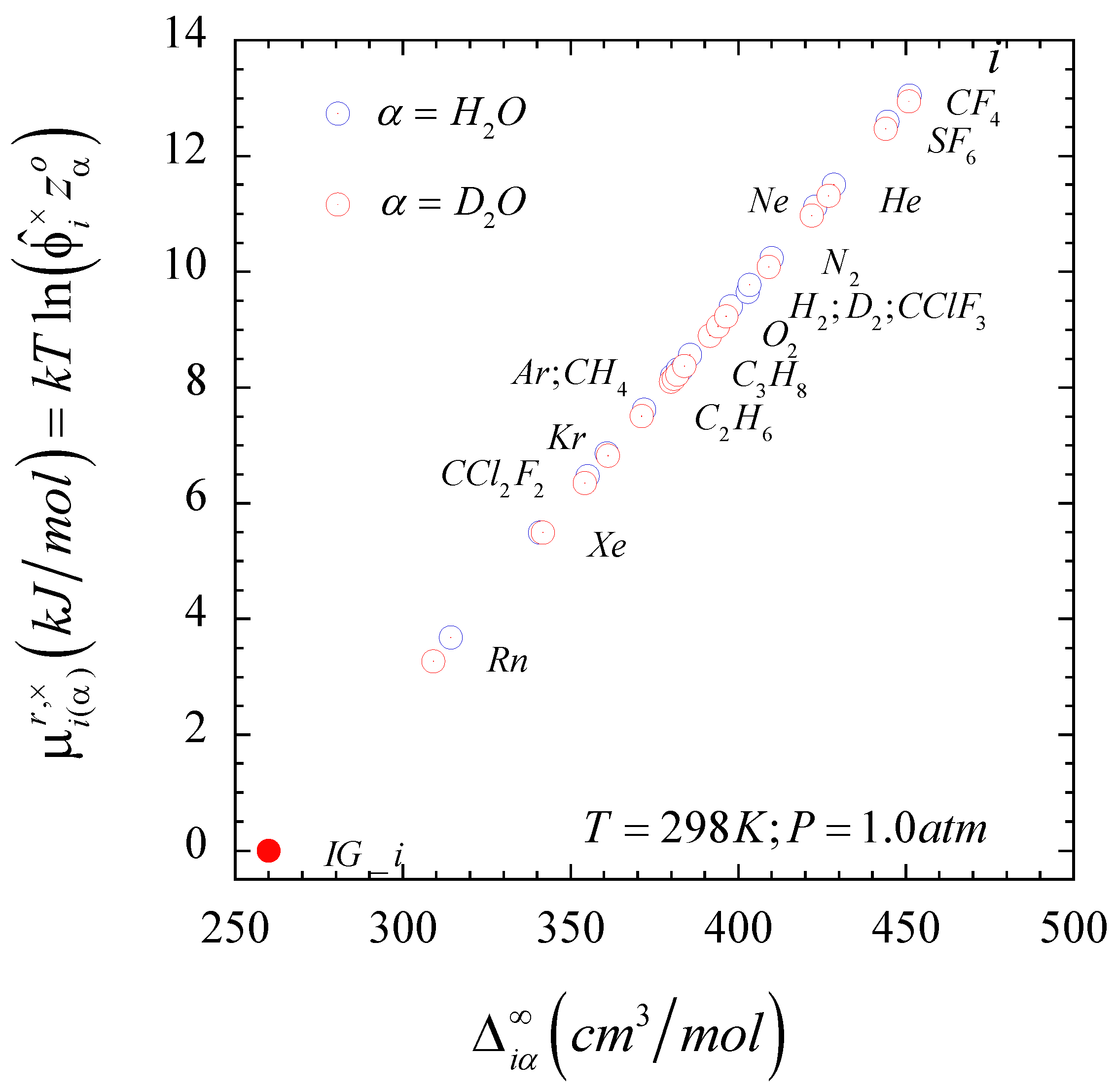
, an observation that we will analyze below. In fact, we should note that the isothermal-isochoric residual chemical potential of the gaseous solutes at infinite dilution in aqueous solutions, μ i ( α ) , r ( T , ρ α o ) , exhibits a linear dependence with the corresponding solute-solvent intermolecular interaction asymmetry function Δ i α ( T , P ) as illustrated in Figure 2 when the α solvent is either light or heavy water at ambient conditions. We can also identify μ I G _ i ( α ) , r ( T , ρ α o ) = 0 at a hypothetical value of the solute-solvent intermolecular interaction asymmetry, i.e., one that differs from the theoretical Δ I G _ i   α ( T , ρ α o ) = G α α o . The reason for this difference resides in the fact that, as demonstrated in Ref. [51], the second-order expansion cannot provide an accurate description of the behavior of non-interacting solutes, i.e., it requires at least a six-order composition expansion. However, because the condition μ I G _ i ( α ) , r ( T , ρ α o ) = 0 also means that γ I G _ i ( α ) L R , ( T , P ) = 1 / z α o , we can determine the hypothetical value of Δ i α , μ i ( α ) , r = 0 so that ln γ I G _ i ( α ) L R , ( T , P ) = 0.5 ρ α o   Δ i α , μ i ( α ) , r = 0 , where Δ i α , μ i ( α ) , r = 0 comprises contributions from the first few infinite dilution composition derivatives of the ln γ I G _ i ( α ) L R ( T , P , x i ) as indicated by Equation S5 in the Supplementary Information document of Ref. [51].
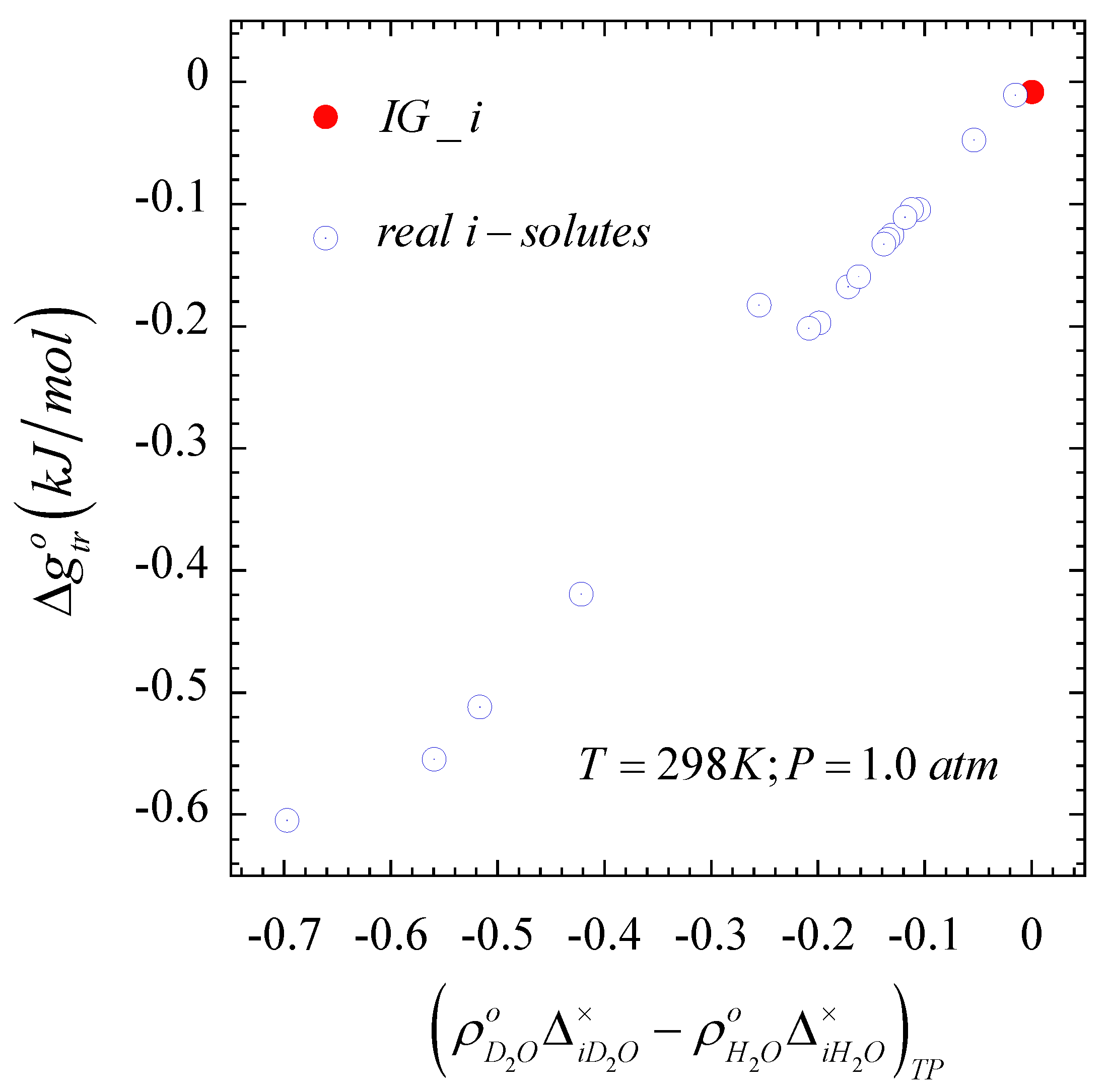
Given the observed linearity in Figure 2, and the definition of the Gibbs free energy of transfer, Equation (10) in the alternative form Δ g t r o ( T , P ) = k T ln ( γ i ( k ) , L R / γ i ( j ) , L R ) T P , we also expect a Δ g t r o ( T , P ) linearly dependent on the difference ( ρ k o Δ i k ρ j o Δ i j ) T P . In fact, the quadratic-composition dependent ln γ i L R ( T , P , x i ) = ln γ i ( j ) , L R ( T , P ) x i 2 that describes accurately the L R nonideal behavior of these solutes [46] leads to Δ g t r o ( T , P ) = 0.5 k T ( ρ k o Δ i k ρ j o Δ i j ) T P with ln γ i ( j ) , L R ( T , P ) = 0.5 ρ j o Δ i j , while the condition ( G i i = G i j = G i k ) T P = 0 for an I G _ i solute translates into ( ρ k o Δ I G _ i k ρ j o Δ I G _ i j ) T P = k T ( ρ k o κ k o ρ j o κ j o ) T P and identified as the red dot in Figure 3. Note also that, while the second-order composition approximation for ln γ i L R ( T , P , x i ) is not accurate for an I G _ i solute as indicated above, we can still identify the I G _ i solute in Figure 3, given that Equation (4) becomes Δ g t r o ( T , P ) = k T ln ( ρ k o / ρ j o ) T P for this solute.
According to the linear behaviors described above, we can alternatively express the solvent effect Δ A K r in terms of the solvation Gibbs free energies Δ G i , α * ( T , P ) as follows,
Δ A k r = A k r I G , k [ Δ G i , k ( T , P ) / k T ln ( f k o / k T ρ k o ) p P ] / β Δ G r = k ( T , P ) + A K r l G i , j [ Δ G i , j ( T , P ) / k T ln ( f j / k T ρ j ) T P ] / β Δ G i = j ( T , P ) = A K r I G i , k ( Δ G i , k / Δ G i = k ) R P + A K r I G i , j ( Δ G i , j / Δ G i = j ) T P + ( A K r I G i , k A K r I G i , j )
where Δ G i , α * ( T , P ) = k T ln ( i , α I S / k T ρ α o ) identifies the solvation Gibbs free energy of the i solute in the α solvent, while Δ G i = α * ( T , P ) = k T ln ( f α o / k T ρ α o ) T P denotes the Gibbs free energy of self-solvation of the α solvent, i.e., μ α o , r ( T , ρ α o ) = k T ln ( ϕ α o z α o ) , for the α = ( j , k ) solvents [40,52]. Likewise, Δ A K r can be equivalently written in terms of the isothermal-isochoric residual chemical potential of the species, μ β , r ( T , ρ α o ) = k T ln ( ϕ ^ β z α o ) , as follows,
Δ A K r = A K r I G _ i , k [ μ i ( k ) , r ( T , ρ k o ) / μ k o , r ( T , ρ k o ) ] + A K r I G _ i , j [ μ i ( j ) , r ( T , ρ j o ) / μ j o , r ( T , ρ j o ) ] + ( A K r I G _ i , k A K r I G _ i , j )
where = o or pure component when β = α , otherwise = describes the condition of infinite dilution of the β solute in an α solvent. This equation represents an alternative answer to question (b) in the Introduction. Finally, Equation (27) can be recast in terms of the Gibbs free energy of transfer of the i solute from the j solvent to the k solvent environments according to Equations (10) and (11), i.e.,
A K r i , k A K r i , j = A K r i , j [ ( μ j o , r / μ k o , r ) ( A K r I G _ i , k / A K r I G _ i , j ) 1 ] + ( A K r I G _ i , k / μ k o , r ) ( μ k o , R μ j o , R Δ g t r o )
which becomes the answer to question (a) in the Introduction as the desirable form of Δ A K r .
Equations (25)–(28) reveal that the solvent effect on the Krichevskii parameter of a solute results from a linear combination of the relative solvation Gibbs free energy of the i solute in the pair of solvents. More specifically, the solvent effect on the magnitude of the Krichesvkii parameter for an i solute becomes directly proportional to the difference of two similar quantities comprising two distinctive terms, i.e., (a) the Krichesvkii parameter for the ideal gas solute in the chosen solvents, and (b) the ratio between the solvation Gibbs free energy of the i solute in the chosen solvents and their self-solvation counterparts. Given the relation between the solvation Gibbs free energy and the species residual free energies, Equation (27), the solvent effect on the Krichevskii parameter can be interpreted as the sum of an ideal gas contribution, ( A K r I G _ i , k A K r I G _ i , j ) , and the difference of A K r I G _ i , α prorated residual free energy ratio μ i ( α ) , r ( T , ρ α o ) / μ α o , r ( T , ρ α o ) for the α = ( j , k ) solvents. Moreover, because the residual quantities measure the contribution of the intermolecular interactions to the thermodynamic properties, the A K r I G _ i , α 
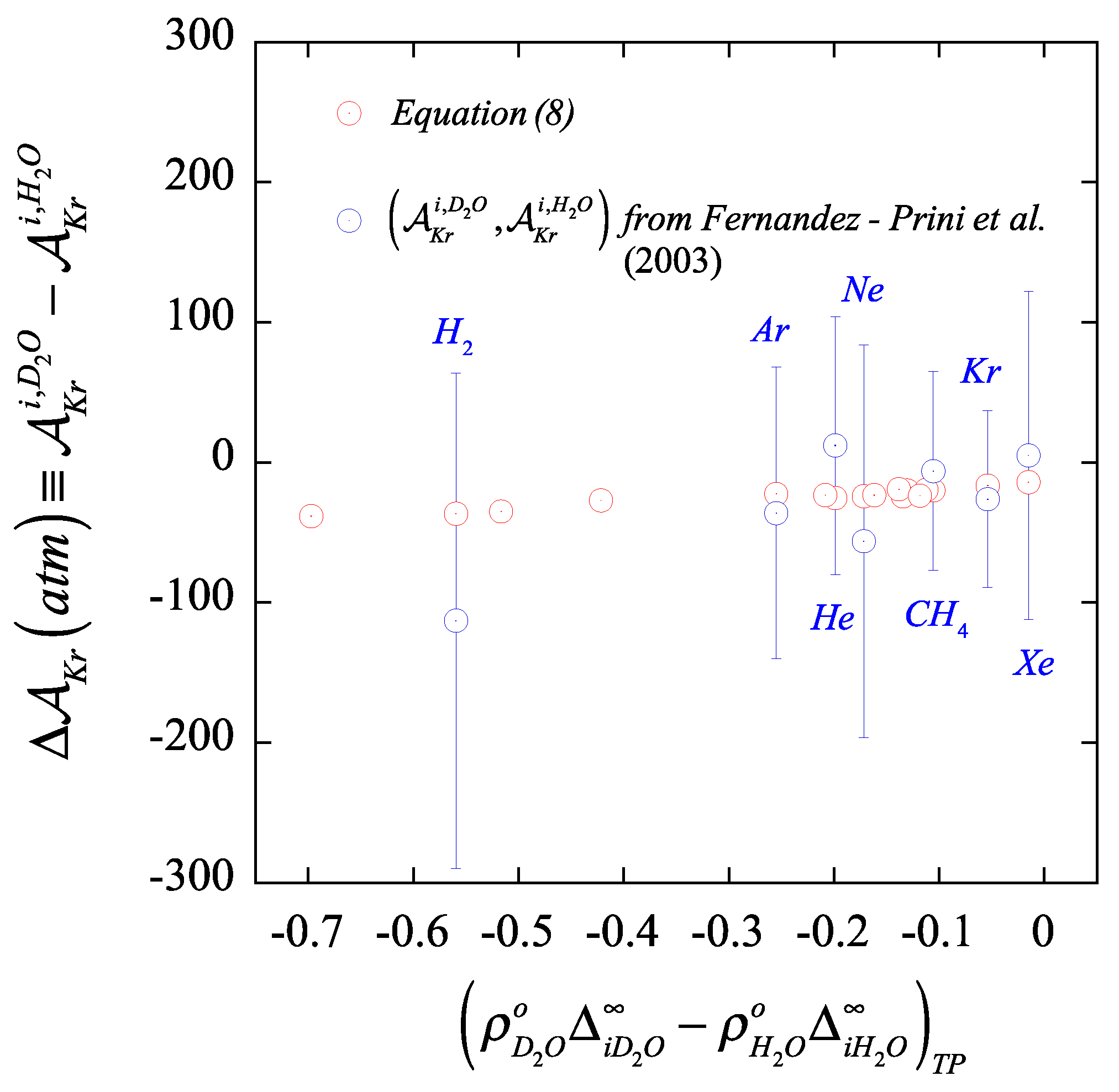
prorated difference conveys the contribution of the difference of solute-solvent intermolecular interaction asymmetries to the solvent effect on the Krichevskii parameter. In fact, according to Equations (10) and (25) as well as the resulting linear behavior in Figure 2 and Figure 3, the solvent effect on the Krichevskii parameter of these gaseous solutes becomes also effectively linear with the difference ( ρ D 2 O o Δ i   D 2 O ρ H 2 O o Δ i   H 2 O ) T P as illustrated in Figure 4.
In summary, Equations (25)–(28) provide alternative direct routes to both (a) a simple test of consistency between the calculated (by any method) Krichevskii parameters of a common i solute in the ( j , k ) pair of solvents through the determination of the standard Gibbs free energy for the transfer of the given i solute from the j solvent to the k solvent, and the standard thermodynamic properties of the two pure solvents, and (b) an accurate evaluation of the effect of the solvent on the Krichevskii parameter of the i solute, i.e., Δ A K r A K r i , k A K r i , j , when we replace the j solvent with the k solvent, avoiding the regression of near-critical properties of the solute in the corresponding solvents as illustrated in Table 4 and Figure 4. In fact, the Δ A K r values reported in Table 4 are the outcome of the derived Equations (8), (27), and (28), which provided precisely the same answer, after invoking the properties from Table 1 and the required thermodynamic properties of the two solvents at ambient conditions from the corresponding equations of state. Among the three theoretically equivalent expressions for Δ A K r , Equations (8), (27) and (28), the first two do not require the reference Krichevskii parameter A K r i , j , and thus, for practical purposes, they might be the preferred routes.
Moreover, in Figure 4, we illustrate the comparison between the solvent H / D isotopic substitution effect on the Krichevskii parameter as determined by the “brute-force” subtraction approach based on the regressed coefficient E of Fernandez-Prini et al. [24] and that from our proposed routes, including the reported uncertainties. This comparison provides clear evidence of the lack of reliability of the “brute-force” approach in the assessment of the H / D isotopic substituted (or for that matter, any solvent) effect from the regression of the Henry law constant and vapor–liquid distribution coefficient of solutes, as we could have anticipated given the challenges behind the measurements at near-critical compared with those at standard ambient solvent environments.

3.6. Solvent H/D−Effect on the Krichevskii Parameter of the Emblematic Ideal Gas Solute

It becomes instructive to analyze the effect of the change of solvent environment on the Krichevskii parameter for an ideal gas solute I G _ i for which we know the answer beforehand, and consequently, to be able to check the validity of the approach. From Equation (4), we obtain
Δ g t r o , I G _ i ( T , P ) = k T ln ( ρ k o / ρ j o ) T P
so that, after introducing (29) and the condition A K r I G _ i , j = k T j , c ρ j , c o into Equation (10), we obtain
A K r i , k = A K r I G _ i , k k T k , c ρ k , c o
which is the expected answer, where we note that the critical conditions of the two solvents are obviously different.

3.7. Solvent H/D−Effect on the Krichevskii Parameter of the Emblematic Case of Lewis-Randall’s Quasi-Ideal Solutions

The mixture of water isotopomers, e.g., D 2 O + H 2 O , falls into the category of quasi-ideal solutions within the Lewis-Randall reference [53]. In fact, in their study of highly dilute aqueous solutions of heavy water, Japas et al. [54] introduced the simplifying assumption of Raoult solution ideality to provide an estimation of the Krichevskii parameter of D 2 O ( i ) in H 2 O ( j ) , and arrived to the following expression in terms of the saturation pressures of the two species, (for a detailed analysis of either Lewis-Randall or Raoult solution ideality of these systems see Appendix B)
( P / x i ) T σ , j ( P i s a t P j s a t ) T σ , j
at T σ , i = T c , i < T c , j and T c , α denotes the critical temperature of the α species. Note that the Krichevskii parameter of an i solute in a j solvent is defined at the critical saturation conditions of the solvent, i.e., A K r i , α = lim T σ , α c r i t i c a l ( P / x i ) T σ , α . Thus, Equation (31) becomes a good guess for the actual A K r D 2 O , H 2 O given that T c , H 2 O T c , D 2 O 4 K .
According to the description of either Hill et al. [49] or Herrig et al. [50] and Wagner and Pruss [48] equations of state for heavy and light water, respectively, we have from Equation (31) that
A K r D 2 O , H 2 O 0.42   M P a
and by the same quasi-ideal approximation for the infinitely dilute light water in heavy-water solvent we can conclude, as discussed in details in Appendix B, that
A K r H 2 O , D 2 O = A K r D 2 O , H 2 O   0.42   M P a
In fact, in Appendix B we have provided a molecular-based argument for the general scenario of a Lewis-Randall ideal solution to demonstrate rigorously that should the mixture of light and heavy water behave ideally, then A K r H 2 O , D 2 O = A K r D 2 O , H 2 O , after assuming for the sake of argument that T c , H 2 O T c , D 2 O .
Obviously, as highlighted by Jancsó and coll. [53,55], these isotopic mixtures exhibit small but non-negligible deviations from ideality, which are usually described by either the simplest symmetric β g E ( x H 2 O ) T P = x H 2 O x D 2 O ln γ L R , , i.e., γ L R , = γ D 2 O , H 2 O L R , = γ H 2 O , D 2 O L R , , or the more realistic asymmetric β g E ( x H 2 O ) T P = x H 2 O 2 x D 2 O ln γ D 2 O , H 2 O L R , + x D 2 O 2 x H 2 O ln γ H 2 O , D 2 O L R , excess Gibbs free energy representation [56]. In this context, we should note that in Table IV of Ref. [57], the authors reported that A K r D 2 O , H 2 O = 0.428   MPa and A K r H 2 O , D 2 O = 0.495   MPa according to the behavior of ( d P c / d x i ) and ( d T c / d x i ) in the evaluation of A K r i , j = ( d P c / d x i ) ( d P σ / d T ) ρ c ( d T c / d x i ) . While A K r D 2 O , H 2 O = 0.428   MPa is in agreement with the sign predicted by the non-ideal solution scenario, A K r H 2 O , D 2 O = 0.495   MPa is at odd. Unfortunately, the authors have not provided any information on the uncertainties for the two composition limiting derivatives involved, though we are aware of the fact that these quantities usually bear large uncertainties that would affect these outcomes [16]. In contrast, in a later report by Bazaev et al. [58], they determined that A K r D 2 O , H 2 O = 0.478   MPa and A K r H 2 O , D 2 O = 0.475   MPa , which are consistent with the theoretical expectations from the ideal solution approximation as discussed in Appendix B.

4. Discussion and Relevant Observations

The proposed approach to the H / D effect on the Krichevskii parameter leads naturally to the assessment of this parameter for binary systems comprising isotopomers. In fact, when the i solute in solution with the original j solvent is simply another j species, i.e., the iconic special case of Lewis-Randall ideal solution, we have A K r i , j = i = 0 , Δ g i , j R ( T , P ) = 0 , Δ g j k o ( T , P ) = k T ln [ ϕ k o ( T , ρ k o ) / ϕ j o ( T , ρ j o ) ] , and Δ g t r o = k T ln [ ϕ ^ j ( T , ρ k o ) / ϕ j o ( T , ρ j o ) ] . Given the resulting A K r i , j = i = 0 , from Equations (3) and (10) we have that the effect of the k solvent on the A K r i , k becomes merely Δ A K r = A K r j , k , i.e.,
A K r j , k = A K r I G _ j , k [ ln ( ϕ ^ j / ϕ k o ) / ln ( ϕ k o z k o ) ] T , ρ k o = A K r I G _ j , k [ ln ( ϕ ^ j / ϕ k o ) / ln ( ϕ ^ k , I G _ k / ϕ k o ) ] T , ρ k o
where the j and k species are simply two isotopomers. Therefore, depending on the solute-solvent intermolecular asymmetry and the fact that usually ( ϕ k o z k o ) 1 at normal conditions, Equation (34) translates into two potential scenarios, either
( ϕ ^ j / ϕ k o ) 1   w i t h   ( ϕ ^ k , I G _ k / ϕ k o ) > 1 { ϕ k o ϕ ^ j ϕ ^ k , I G _ k A K r j , k > 0
or,
( ϕ ^ j / ϕ k o ) 1   w i t h   ( ϕ ^ k , I G _ k / ϕ k o ) 1 { ϕ ^ j ϕ k o ϕ ^ k , I G _ k A K r j , k < 0
By noting that when the k species is an ideal gas, ϕ ^ k , I G _ k z k o , 1 = ( k T ρ k o / P ) 1 [30], so that for the case of mixtures of light ( j species) and heavy water ( k species) we have ϕ ^ j ( T , P ) ϕ k o ( T , P ) , consequently, we expect A K r j , k < 0 according to Equation (36). Otherwise, when ϕ ^ j ( T , P ) ϕ k o ( T , P ) , we expect A K r j , k > 0 according to Equation (35). In other words, Equations (35) and (36) indicate that the sign of the Krichevskii parameter of an isotopic j solute in an isotopic k solvent will be decided by either ( γ j L R , ϕ j o ) T P ϕ k o ( T , P ) or γ j L R , ( T , P ) ( ϕ k o / ϕ j o ) T P conditions, where A K r j , k < 0 , A K r j , k = 0 , and A K r j , k > 0 will be the outcome for the upper inequality, the middle equality and the lower inequality, respectively.
At this point, it is worth highlighting the subtle effect of the small perturbations of the solute-solvent intermolecular interaction asymmetry Δ H 2 O   D 2 O around zero, i.e., the Lewis-Randall (Raoult) solution ideality [59], on the non-ideality of these aqueous systems. On the one hand, the D 2 O + H 2 O system described as a slightly non-ideal solution characterized by the excess Gibbs free energy β g E ( x H 2 O ) T P = x H 2 O x D 2 O ln γ L R , with γ D 2 O , H 2 O L R , = γ H 2 O , D 2 O L R , = γ L R , , as suggested by Jancsó et al. [53], leads to
( ϕ ^ H 2 O , D 2 O / ϕ H 2 O o   ) T P = ( ϕ ^ D 2 O , H 2 O / ϕ D 2 O o   ) T P ( ϕ ^ H 2 O , D 2 O / ϕ D 2 O o ) T P = ( ϕ ^ D 2 O , H 2 O / ϕ H 2 O o ) T P ( T , P )
after considering the definition γ i , j L R , ( T , P ) = ( ϕ ^ i , j / ϕ i o ) T P with = ( ϕ H 2 O o / ϕ D 2 O o ) T P . Consequently, as the solute-solvent interaction asymmetry Δ i j ( T , P ) vanishes, we have that lim Δ H 2 O   D 2 O 0 γ H 2 O , D 2 O L R , = lim Δ D 2 O   H 2 O 0 γ D 2 O , H 2 O L R , = 1 . Therefore, the reference to the Lewis-Randall (Raoult) solution ideality for the description of the behavior of the D 2 O + H 2 O system, i.e., Δ H 2 O   D 2 O = Δ D 2 O   H 2 O = 0 , represents the equivalent limiting behavior,
G H 2 O   H 2 O o = G D 2 O   D 2 O o = G H 2 O   D 2 O = G H 2 O   H 2 O = G D 2 O   D 2 O 0
as if the light and heavy water behaved identically, leading to = 1 , and consequently to A K r H 2 O , D 2 O = A K r D 2 O , H 2 O = 0 , which is obviously not consistent with the actual case for the water isotopomers. In fact, the symmetric nature of the β g E ( x H 2 O ) T P = x H 2 O x D 2 O ln γ L R , description for the non-ideality of these mixtures is neither agreeing with the actual ( T , P ) 1 evidence, nor being compatible with the general Lewis-Randall (Raoult) behavior discussed in Appendix B which leads to A K r H 2 O , D 2 O = A K r D 2 O , H 2 O .
On the other hand, because the two water isotopomers exhibit slightly different thermodynamic behaviors, e.g., ( ϕ H 2 O o / ϕ D 2 O o ) T P 1 , we might expect a marginally asymmetric isothermal-isobaric composition representation for its excess Gibbs free energy. In other words, instead of the simple symmetric B4 form, we could have a more realistic Margules-type representation, i.e., β g E ( x H 2 O ) T P = x H 2 O 2 x D 2 O ln γ D 2 O , H 2 O L R , + x D 2 O 2 x H 2 O ln γ H 2 O , D 2 O L R , [56], so that [60]
ρ H 2 O o Δ D 2 O   H 2 O = 4 ln γ D 2 O , H 2 O L R , 2 ln γ H 2 O , D 2 O L R , ρ D 2 O o Δ H 2 O   D 2 O = 4 ln γ H 2 O , D 2 O L R , 2 ln γ D 2 O , H 2 O L R ,
and consequently, lim Δ H 2 O   D 2 O 0 γ H 2 O , D 2 O L R , = lim Δ D 2 O   H 2 O 0 γ D 2 O , H 2 O L R , = 1 , leading to
lim Δ H 2 O   D 2 O 0 ( ϕ ^ H 2 O , D 2 O / ϕ D 2 O o ) T P = ( ϕ H 2 O o / ϕ D 2 O o ) T P lim Δ H 2 O   D 2 O 0 γ H 2 O , D 2 O L R , = 1 lim Δ D 2 O   H 2 O 0 ( ϕ ^ D 2 O , H 2 O / ϕ H 2 O o ) T P = ( ϕ D 2 O o / ϕ H 2 O o ) T P lim Δ D 2 O   H 2 O 0 γ D 2 O , H 2 O L R , = 1 1
This analysis indicates that the relative magnitude of the two activity coefficients at infinite dilution, γ H 2 O , D 2 O L R , and γ D 2 O , H 2 O L R , , decides the sign of the corresponding Krichevskii parameters. In fact, after invoking Equations (35) and (36), and according to the equations of state for light [48] and heavy water [49,50], = ( ϕ H 2 O o / ϕ D 2 O o ) T P o 1.15 , then we can reach the following conclusions,
γ D 2 O , H 2 O L R , > A K r D 2 O , H 2 O > 0 1 γ D 2 O , H 2 O L R , < A K r D 2 O , H 2 O < 0
and,
1 γ H 2 O , D 2 O L R , > 1 A K r H 2 O , D 2 O > 0 γ H 2 O , D 2 O L R , < 1 A K r H 2 O , D 2 O < 0
Notably, the available literature provide at least two sets of experimental data for the Krichevskii parameters A K r H 2 O , D 2 O and A K r D 2 O , H 2 O , i.e., those from Abdulkadirova et al. [57] and from Bazaev et al. [58] The first one, given in their Table IV, indicates that A K r H 2 O , D 2 O A K r D 2 O , H 2 O > 0 , which would suggest that the two activity coefficients at infinite dilution are different and follow the relation γ D 2 O , H 2 O L R , > > ( 1 / γ H 2 O , D 2 O L R , ) . In contrast, the second source indicates that A K r H 2 O , D 2 O < 0 while A K r D 2 O , H 2 O > 0 , resulting in two different activity coefficients at infinite dilution obeying the relation γ D 2 O , H 2 O L R , >   < ( 1 / γ H 2 O , D 2 O L R , ) . Therefore, while the two referred sources agreed on that A K r D 2 O , H 2 O > 0 , they are at odds on the sign of A K r H 2 O , D 2 O . Moreover, while the two references also agree with the outcome from the ideal solution approximation given by Japas et al. [54], i.e., A K r D 2 O , H 2 O > 0 as in Equation (32), only does Bazaev et al. [58] match the A K r H 2 O , D 2 O < 0 counterpart.
We should emphasize that the agreement/disagreement observed in these datasets must be taken with caution given not only the approximated nature of the quasi-ideality approach and its inherent inconsistency as discussed above, but also the magnitude of the H / D effect relative to the size of the uncertainties in the experimentally measured coefficients associated with the calculation of the corresponding Krichevskii parameters. In fact, we should also note that the A K r D 2 O , H 2 O and A K r H 2 O , D 2 O are about two orders of magnitude smaller than the typical values for aqueous non-electrolyte solutes, e.g., see tabulation in Ref. [16], making their accurate experimental determination extremely challenging.
Yet, the most important aspects of the observed disparity of results are their microscopic (solvation) interpretation and macroscopic (thermodynamic) modeling consequences. Considering its thermodynamic representation, A K r i , α = lim T , ρ α o c r i t i c a l ( ρ α o υ ^ i / κ α o ) , and the positive definite nature of the molar volume and isothermal compressibility of the pure solvent, it becomes obvious that the sign of A K r i , α is defined by the sign of the diverging partial molar volume of the solute, υ ^ i , a crucial feature for the appropriate interpretation of solvation phenomena in highly compressible environments [1,61]. In fact, the observed solvent H / D effects on the Krichevskii parameter of a solute can be interpreted in terms of the solute’s ability to perturb the solvent microstructure, given that lim T , ρ α o c r i t i c a l ( P / x i ) T ρ = A K r i , α , and the pressure perturbation ( P / x i ) T ρ is directly linked to the structure making/breaking parameter for a general dissociative ( ν = 1 for non-dissociative) i solute [62,63], as follows
S i α ( T , P ) = ν 1 κ α o ( P / x i ) T ρ
where κ α o denotes the isothermal compressibility of the pure α solvent. Consequently, we can immediately conclude that,
A K r i , α = ν lim T , ρ α o c r i t i c a l ( S i α / κ α o )
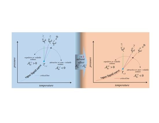
The significance of Equation (44) becomes evident after noting that the sign of the pressure perturbation upon solute solvation ( P / x i ) T ρ has been key in the characterization of the solvation behavior of solutes in near-critical solvents, so that according to Equation (43) an i solute behaves as a structure-maker in an α solvent environment when the system exhibits a ( P / x i ) T ρ < 0 [62], and the solute is depicted as non-volatile [2] or attractive [64]. Conversely, an i solute behaves as a structure-breaker in an α solvent environment when the system responds with a ( P / x i ) T ρ > 0 [62], and the solute is described as volatile [2] or weakly attractive and repulsive [64] in the jargon of supercritical fluid solutions [65,66].
More importantly, from the fundamental expression given by Equation (43), we can split S i α ( T , P ) into its solvation (i.e., short-range local density perturbation, S R ) contribution while isolating its diverging (i.e., long-range or compressibility driven, L R ) contribution associated with the propagation of the density perturbation as follows [8],
S i α ( T , P ) = ν 1 κ α o , I G ( P / x i ) T ρ S i α ( S R ) ν 1 κ α o , R ( P / x i ) T ρ S i α ( L R )
In Equation (45), we identify κ α o , I G = ( ρ α o k T ) T P 1 as the ideal gas compressibility at the prevailing state conditions, and κ α o , R ( T , P ) = κ α o κ α o , I G as the corresponding isobaric-isothermal residual isothermal compressibility. Therefore, from Equations (43) and (45) we immediately find the desired explicit expression for the solvation finite contribution,
S i α ( S R ) = ( κ α o , I G / κ α o ) S i α
whose divergent compressibility-driven contribution becomes,
S i α ( L R ) = ( κ α o , R / κ α o ) S i α
Moreover, as demonstrated in Appendix C, the solvation and compressibility-driven contributions to the structure making/breaking parameter S i α ( T , P ) are related as follows,
S i α ( L R ) = S i α , I G _ i S i α ( S R )
with S i α , I G _ i = 1 ρ α o k T κ α o . Equation (48) tells us that the long-range contribution to the structure parameter of any real solute in an α solvent, S i α ( L R ) , becomes proportional to its short-range counterpart S i α ( S R ) through the negative value of the structure parameter of the ideal gas i solute in the real α solvent environment at the prevailing state conditions, S i α , I G _ i ( T , P ) . Consequently, from Equations (44) and (A41) of the Appendix C, we finally arrive to the following fundamental identity,
A K r i , α = ν A K r I G _ i , α lim T , ρ α o c r i t i c a l S i α ( S R )
so that, the solvent effect on the Krichevskii parameter becomes,
Δ A K r = ν [ A K r I G _ i , k lim T , ρ k o c r i t i c a l S i k ( S R ) A K r I G _ i , j lim T , ρ j o c r i t i c a l S i j ( S R ) ] = ν k [ T k , c ρ k , c o S i k , c ( S R ) T j , c ρ j , c o S i j , c ( S R ) ]
The identity in Equation (49) emphasizes that the Krichevskii parameter of an i solute ability to perturb the α solvent environment is simply that of the corresponding ideal gas solute I G _ i prorated by ( v ) times the short range (finite) contribution to the structure making/breaking parameter at critical conditions. Any increase (decrease) in the i solute ability to perturb the α solvent environment as a structure-making effect, S i α > 0 , will translate into a more (less) negative A K r i , α . Otherwise, any increase (decrease) in the i solute ability to perturb the α solvent as a structure-breaking effect, S i α < 0 , will translate into a more (less) positive A K r i , α . Likewise, when the i solute is identical to the k solvent ( D 2 O ), the effect of the j solvent ( H 2 O ) will manifest as slightly positive, i.e., A K r D 2 O , H 2 O 0 (see (A44) in Appendix D). In other words, according to the analysis above, a D 2 O molecule as a solute will exhibit a structure-breaking behavior in the solvent H 2 O environment, S D 2 O   H 2 O ( S R ) < 0 , while a H 2 O molecule as a solute will induce a structure-making perturbation of the solvent D 2 O environment, S H 2 O   D 2 O ( S R ) > 0 (i.e., A K r H 2 O , D 2 O 0 according to (A43) in Appendix D).

5. Final Remarks and Outlook

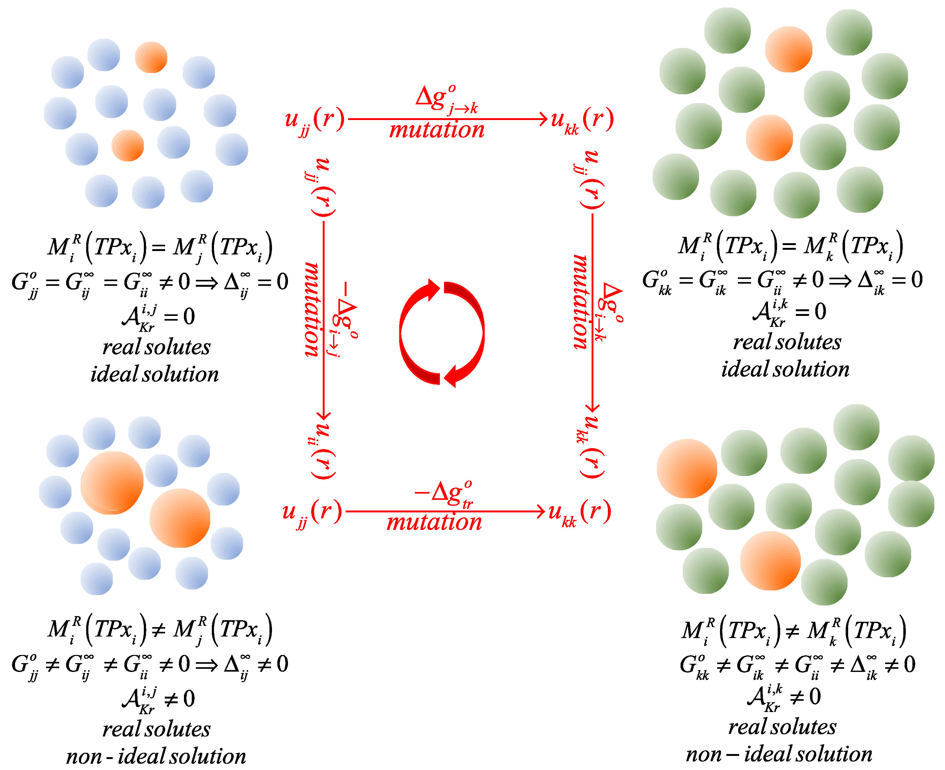
In this work we have discussed the solvent effect on the Krichevskii parameter of an i solute in a k solvent, A K r i , k , and addressed its accurate determination when we know either (a) not only the solvation behavior of the i solute in a j solvent but also, its Krichevskii parameter A Kr i , j , or (b) the solvation behavior of the i solute in both solvents as well as the Gibbs free energy of transfer of the i solute between the two solvents. For that purpose, we first proposed a general molecular thermodynamic approach based on a Gibbs free energy cycle at standard state conditions, and then, we applied it to the determination of the H / D isotopic substitution effect on the Krichevskii parameter of gaseous solutes in light and heavy water.
Although theoretically equivalent, the choice among the resulting Equations (8), (27) and (29) would depend on the non-trivial condition of accuracy of the available data for the Krichevskii parameter A K r i , j of the i solute in the reference j solvent. Consequently, it becomes more fruitful to assess directly the solvent effect as Δ A K r , Equations (8) and (27), and after validating the accuracy of A K r i , j , proceed with the evaluation of A K r i , k = Δ A K r + A K r i , j .
The proposed scheme, developed around a fundamentally based solvation formalism of dilute solutions, identifies the links between the standard solvation Gibbs free energy of the i solute in the two participating solvent environments and the resulting Krichevskii parameters, thorough the linear relation between the latter and the standard solvation Gibbs free energy of the solute. Additionally, it provides a novel microstructural interpretation of the solvent effect on the Krichevskii parameter through the rigorous characterization of the critical solvation as described by a finite unambiguous structure making/breaking parameter S i α ( S R ) of the i solute in the pair of α solvent environments. The molecular thermodynamic foundations of the proposed approach, combined with the involvement of accurate standard solvation properties, provide a broader and encouraging outlook on the understanding, and consequent interpretation, of the solvent effect on the Krichevskii parameter of any solute in any solvent environment.

Supplementary Materials

The following supporting information can be downloaded at: https://www.mdpi.com/article/10.3390/liquids2040028/s1, SI-1. Alternatives solvation cycle paths for the study of the transfer Gibbs free energy of an infinitely dilute solute, and SI-2. Determination of the standard Gibbs free energy of hydration of hydrogen isotopes in light and/or heavy water.

Author Contributions

Conceptualization, A.A.C.; methodology, A.A.C.; formal analysis, A.A.C.; resources, O.D.C.; writing—original draft preparation, A.A.C.; writing—review and editing, O.D.C. All authors have read and agreed to the published version of the manuscript.

Funding

This research received no external funding.

Data Availability Statement

Not applicable.

Conflicts of Interest

The authors declare no conflict of interest.

Nomenclature

Symbols
A K r , A K r i , j Krichevskii parameter of an i solute in a j solvent, i.e., lim T , ρ j o c r i t i c a l ( P / x i ) T ρ
C α β ( T , P ) direct correlation function integral, aka DCFI, for the α β interactions at the ⊗ conditions, either infinite dilution ∞ or pure component o
D C F I direct correlation function integral
f i ( T , P , x i ) fugacity of the i species
α ( T , P ) isobaric-isothermal function defined by Equation (6)
G α β ( T , P ) Kirkwood-Buff integral for the α β interactions at the ⊗ conditions, either infinite dilution ∞ or pure component o
i , j I S ( T , P ) Henry’s law constant of an i species in a j solvent given by i , j I S ( T P ) = f i o ( T P ) γ i L R , ( T P )
k Boltzmann constant
K B Kirkwood-Buff
κ j o ( T , P ) isothermal compressibility of the pure j solvent
K D ( T , P ) vapor-liquid solute distribution coefficient
M W α molar weight of an α species
m i o reference molality of an i solute
N α number of molecules of an α species
P system pressure
P i ( a ) , R generic isobaric-isothermal residual property of an infinitely dilute i species in an α solvent
P ^ i ( T , P ) generic partial molar property of an infinitely dilute i species
S i , j ( T , P ) structure making/breaking parameter of an infinitely dilute i species in a j solvent
S R , L R short- and long-range contributions to the Kirkwood-Buff integral according to the Ornstein-Zernike equation
T C F I total correlation function integral, aka Kirkwood-Buff integral
T , P state conditions defined by the system temperature and pressure
T , ρ state conditions defined by the system temperature and density
V ( T , P , x i ) system volume at the specified state conditions and composition
υ ^ i ( T , P , x i ) partial molar volume of the i species
x i liquid phase composition defined by the mole fraction of the i species
z j o ( T , P ) compressibility factor P / ρ j o k T for the pure j solvent
Δ h G i , j ( T , P ) standard solvation Gibbs free energy of the i solute in the j solvent
Δ g t r o ( T , P ) solvation Gibbs free energy of transfer of an infinitely dilute i solute between two solvent environments
Δ G i * ( T , P ) σ solvation Gibbs free energy according to Ben-Naim’s definition
Δ i j ( T , P ) linear combination of Kirkwood-Buff integrals related to the non-ideality of the dilute solution, i.e., ( G i i + G j j o 2 G i j ) T P
ϕ ^ i ( T , P , x i ) partial molar fugacity coefficient of the i species
( ) a general function
γ i L R ( T , P , x i ) Lewis-Randall’s activity coefficient of the i species, i.e., ϕ ^ i ( T , P , x i ) / ϕ i o ( T , P )
μ i R ( T , P , x i ) isobaric-isothermal residual chemical potential of the i species at the specified state conditions and composition
μ i r ( T , ρ , x i ) isochoric-isothermal residual chemical potential of the i species at the specified state conditions and composition
ρ ( T , P , x i ) molar density of the system at the specified state conditions and composition
Sub- and super-scripts
c critical condition for the pure j solvent
o pure component
infinite dilution
i solute species
I S ideal solution
j , k solvent species
L R Lewis-Randall
I G ideal gas condition
I G _ i special case of solute as an ideal gas i species
L R I S special case of Lewis-Randall ideality when ( G i i = G i j = G j j o ) T P
R residual property at constant ( T , P , x i )
r residual property at constant ( T , ρ , x i )

Appendix A. Relation among Solvation Gibbs Free Energy Expressions

The standard Gibbs free energy of hydration (solvation) Δ h G i ( T , P o ) of a solute species is the isothermal-isobaric change of free energy required to transfer the species from an ideal gas environment, at P o (either 1.0   a t m [29,67], or 0.1   MPa [37,38]) and temperature T , into the solvent environment to form a hypothetical solution of unit molality, i.e., [29]
Δ h G i ( T , P o ) = k T ln ( f ^ i / f i o , I G ) T P o + k T ln ( m i o M W j ) = k T ln ( i , j I S / P ) T P o + k T ln ( m i o M W j ) = k T ln ( i , j I S / f j o ) T P o + k T ln ( f j o / P ) T P o + k T ln ( m i o M W j )
where m i o = 1.0   m o l / k g denotes the unit molality of the i solute in the j solvent of molecular weight M W j , while i , j I S ( T , P ) and f j o ( T , P ) represent the corresponding Henry’s law constant of the i solute and the fugacity of the j solvent at the prevailing state conditions, respectively. Note that the first term, k T ln ( i , j I S / f j o ) T P in (A1) describes the difference of residual Gibbs free energy between the infinite dilute solute and the original solvent species in the alchemical process depicted in Figure 1 of Ref. [4], where the superscripts r and R denote residual properties at fixed system density or pressure, i.e.,
k T ln ( i , j I S / f j o ) T P = μ i , r ( T , ρ ) μ j o , r ( T , ρ ) = μ i , R ( T , P ) μ j o , R ( T , P )
with P a r , ( T , ρ ) = P a R , ( T , P ) + k T   ln ( P / k T ρ ) , where represents either an infinite dilution, , or a pure component, o , condition. After identifying f j o ( T , P ) = i , j I S , L R I S ( T , P ) , from (A1) and (A2), [30] we also have that
k T ln ( i , j I S / f j o ) T P o = Δ h G i ( T , P o ) k T ln ( ϕ j o m i o M W j ) T P o
Note that, whenever the Henry’s law constants are given at the saturation conditions T σ , then
k T ln ( i , j I S / f j o ) T P σ = Δ h G i ( T , P o ) k T ln ( m i o M W j ) + k T ln [ P o / f j o ( T , P σ ) ]
where we assume that i , j I S ( T , P o ) i , j I S ( T , P σ ) given the negligibly small Poynting correction under these conditions. In fact, we can rewrite (A4) as follows,
k T ln ( i , j I S / f j o ) T P σ = ( Δ h G i Δ h G i = j ) T P o
after invoking Equation (21), and recognizing that f j o ( T , P o ) / f j o ( T , P σ ) 1 at ambient conditions. Moreover, from (A5) and its corresponding expression for an ideal gas solute, we find that,
k T ln ( i , j I S / k T ρ j o ) T P σ = k T ln ( i , j I S / i , j I S , I G _ i ) T P σ = Δ G i * ( T , P ) σ = ( Δ h G i Δ h G I G _ i ) T P o
Then, from (A4)–(A6) we obtain,
Δ G i * ( T , P ) σ = ( Δ h G i Δ h G I G _ i ) T P o = k T ln ( ϕ ^ i z j o ) T P σ = μ i r , ( T , ρ j o ) σ
Δ G i = j * ( T , P ) σ = ( Δ h G i = j Δ h G I G _ i ) T P o = k T ln ( ϕ j o z j o ) T P σ = μ j r , o ( T , ρ j o ) σ
Alternatively, (A5)–(A7) provide the following relations,
k T ln ( i , j I S / f j o ) T P σ = ( μ i , R μ j o , R ) σ = Δ G i * ( T , P ) σ k T ln ( ϕ j o z j o ) σ = k T ln ( ϕ ^ i z j o ) σ k T ln ( ϕ j o z j o ) σ = ( μ i , r μ j o , r ) σ
so that, from (A4), we obtain
Δ h G I G _ i ( T , P σ ) = k T ln ( z j , σ o P o / P σ ) + k T ln ( m i o M W j )
and from (A7) and (A10), we find
μ i r , ( T , ρ j o ) = Δ h G i ( T , P o ) + k T ln ( z j , σ o P o / P σ ) k T ln ( m i o M W j )
Note also that, following the original definition, such as in Refs. [68,69], we have that
Δ μ i ( T , P ) σ = k T ln ( i , j I S / P o ) T P σ = k T ln ( i , j I S / k T ρ j o ) T P σ + k T ln ( P σ / P o z j , σ o ) = Δ G i * ( T , P ) σ + k T ln ( P σ / P o z j , σ o )
Finally, we consider the low-pressure gas solubility scenario as described by Wilhelm et al. [39,67] i.e.,
Δ s o l μ i = ( μ i s a t μ i o , I G ) T P o = k T ln ϕ ^ i s a t ( T , P o , x i s a t ) = k T ln γ i L R , s a t ( T , P o , x i s a t ) + k T ln ϕ i o ( T , P o ) k T ln γ i L R , s a t ( T , P o , x i s a t ) k T ln x i s a t ( T , P o )
where the equivalence and validity of the approximation in the (A13) has been discussed elsewhere [47] so that, we can identify the following link [45],
Δ G i * ( T , P ) σ Δ s o l μ i k T ln ( k T ρ j o / P o ) = k T ln ( γ i L R , P o / k T ρ j o ) = k T ln γ i L R , ( T , P o ) + k T ln ( z j , σ o P o / P σ )
given that the negligible pressure difference ( P σ P o ) . Moreover, from (A1) and (A14), we find
Δ h G i ( T , P o ) = k T ln γ i L R , ( T , P o ) k T ln ( m i o M W j )
Therefore, (A1)–(A15) provide the links among the three frequently quoted changes of Gibbs free energy in the solvation process.

Appendix B. Krichevskii Parameter of Solutes in Quasi-Ideal Solutions

The typical case of Lewis-Randall’s quasi-ideality is represented by mixtures of isotopic forms of the same compound such as H 2 O + D 2 O [53,55]. For that purpose, Japas et al. [54] introduced the simplifying assumption of (Lewis Randall and/or Raoult) solution ideality, i.e., [70]
P ( T , x i ) = ( P i s a t γ i L R x i ) / Φ i + ( P j s a t γ j L R x j ) / Φ j
where Φ α ( P , T , y α ) represents the pressure correction to the fugacity coefficient of the α species in the vapor phase, i.e.,
Φ α = ( ϕ ^ α / ϕ ^ α s a t ) exp ( β P α s a t P υ α d P )
Note that for the low density vapor (A17) can be written in terms of second virial coefficients as follows,
Φ α = exp [ β ( B α α υ α ) ( P P α s a t ) + β P y β 2 δ α β ]
with δ α β = 2 B α β B α α B β β , where B α β ( T ) defines the second virial coefficient for the α β pair interactions.
Now, according to Jancsó et al. [53], the quasi-ideal behavior of the H 2 O + D 2 O mixture could be described by the (Margules-Porter) quadratic excess Gibbs free energy expression,
β g E ( T , P , x i ) = A x i x j = ln γ L R , x i x j
with γ i L R , = γ j L R , = γ L R , , and A = 0.5 ρ j o ( G j j o + G i i 2 G i j ) [46]. Therefore, if we follow Japas et al.’s assumptions [54] i.e., we set Φ α = 1 and γ α L R , = 1 , so that from (A16) we obtain,
( P / x i ) T σ ( P i s a t P j s a t ) T α
Note that, under the same ideal-behavior approximations we expect, at the x j 0 limit, that
( P / x j ) T σ ( P j s a t P i s a t ) T σ
Consequently,
( P / x i ) T σ = ( P / x j ) T σ
A more rigorous way to tackle this “quasi-ideal” case is through the analysis of the solute-solvent intermolecular interaction asymmetry using the Kirkwood-Buff formalism [71]. In fact, if we assume ideality, then [59]
Δ i j L R I S ( T , P , x i ) = G i i I S + G j j I S 2 G i j I S = 0
where the trivial situation will indicate that G α β I S ( T , P , x ) = 0 for all pairs of α β interactions, i.e., a system where the solvent and the solute are differentiated only by their labels. However, we are interested in the general case, i.e.,
( G i i I S G i j I S ) + ( G j j I S G i j I S ) = 0 = ( A + A + ) T P x = 0 A ( T , P , x i ) = A + ( T , P , x i )
with A ( T , P , x i ) 0 and A + ( T , P , x i ) 0 , leading to the following expressions for the species partial molar volumes from the Kirkwood-Buff formalism [71],
ρ υ i I S = 1 + ρ j ( G j j I S G i j I S )
ρ υ j I S = 1 + ρ i ( G i i I S G i j I S )
From (A25) and (A26),
υ i I S / υ j I S = [ 1 + ρ j ( G j j I S G i j I S ) ] / [ 1 + ρ i ( G i i I S G i j I S ) ] = ( 1 + ρ j A + ) / ( 1 ρ i A + )
or its alternative form,
υ i I S ( 1 ρ i A + ) = υ j I S ( 1 + ρ j A + )
whose limiting behavior read,
lim ρ i 0 υ i I S = υ i I S , = υ j I S , o + A + o ( x i = 0 ) ; A + o = ( G j j I S , o G i j I S , ) x i = 0 lim ρ j 0 υ j I S = υ j I S , = υ i I S , o A + ; A + ( x j = 0 ) = ( G j j I S , G i j I S , ) x j = 0
Likewise, we provide the asymptotic behavior of the infinite dilution species partial molar volumes, i.e.,
lim ( T , P ) j c r i t ( υ i I S , / κ j o ) = lim ( T , P ) j c r i t ( A + o / κ j o ) lim ( T , P ) i c r i t ( υ j I S , / κ i o ) = lim ( T , P ) i c r i t ( A + / κ i o )
Note that, given (A24), we find that
A + o = A o A + = A } { A + o = A A o = A + } A o = A + o = A = A +
Therefore, from (A30) and (A31), we conclude that,
lim ( T , P ) c r i t ( υ i I S , / κ j o ) = lim ( T , P ) j c r i t ( A + o / κ j o ) = lim ( T , P ) j c r i t ( G j j I S , o G i j I S , ) x i = 0 / κ j o lim ( T , P ) i c r i t ( υ j I S , / κ i o ) = lim ( T , P ) i c r i t ( A + / κ i o ) = lim ( T , P ) i c r i t ( G j j I S , G i j I S , ) x j = 0 / κ i o = lim ( T , P ) i c r i t ( G j j I S , o G i j I S , ) x i = 0 / κ i o
and thus, within the ideality condition (A23), and after considering that T c , j T c , i , the two Krichevskii parameters become related as follows,
A K r i , j = A K r j , i
In other words,
υ D 2 O I S , H 2 O     c r i t i c a l i t y + κ H 2 O o ρ H 2 O o υ D 2 O I S , / κ H 2 O o = A K r D 2 O , H 2 O > 0 υ H 2 O I S , D 2 O     c r i t i c a l i t y κ D 2 O o ρ D 2 O o υ H 2 O I S , / κ D 2 O o = A K r H 2 O , D 2 O < 0
where α     c r i t i c a l i t y means that the property on the left scales asymptotically as the property of the right with the indicated sign.
Note that, as the actual T c , j a p p r o a c h e s T c , i , the ideality condition given by (A24) becomes more restrictive and approaches A ( T , P , x i ) = A + ( T , P , x i ) = 0 , or alternatively, G i i I S = G i j I S = G j j I S 0 . This is the special case of null solute–solvent intermolecular asymmetry, Δ i j L R I S ( T , P , x ) , and the system behaves as a pure fluid.

Appendix C. Relation between the Krichevskii Parameter A K r and the Structure Making/Breaking Parameter S i α

Note also that the isothermal-isochoric rate of change of pressure ( P / x i ) T ρ can also be written as ( P / x β ) T ρ = ν ρ α o ( C α α o C β α ) / κ α o , I G [28], where C β α ( T , P ) 4 π 0 c β α ( r ) r 2 d r defines the DCFI for the β α type of interactions at the prevailing ( T , P ) state conditions and composition, i.e., = o for the pure component and = for the infinite dilution [1]. Thus, after invoking the following macroscopic interpretation for the DCFI [13],
C α α o ( T , P ) = υ α o [ 1 ( ν υ α o / υ ^ i , I G _ i ) ]
C i α ( T , P ) = υ α o [ 1 ( υ ^ i / υ ^ i , I G _ i ) ]
so that,
( P / x i ) T ρ = ν k T ρ α o ( υ ^ i ν υ α o ) / υ ^ i , I G _ i = ν ( υ ^ i ν υ α o ) / ( υ ^ i , I G _ i κ α o , I G )
Therefore, from Equations (41) and (A37), we find
S i α ( S R ) = ( υ ^ i ν υ α o ) / υ ^ i , I G _ i = ( υ ^ i ν υ α o ) / ( ν k T κ α o )
leading straightforwardly to,
S i α ( L R ) = ( υ ^ i ν υ α o ) ( [ 1 / υ ^ i , I G _ i ] [ 1 / ν υ α o ] )
where κ α o , I G = ( k T ρ α o ) 1 and υ ^ i , I G _ i = ν k T κ α o so that,
S i α ( L R ) = ( k T ρ α o κ α o 1 ) S i α ( S R ) = S i α , I G _ i S i α ( S R )
Equation (A40) tells us that the long-range contribution to the structure parameter of any real solute, S i α ( L R ) , regardless of the value of ν , becomes proportional to its short-range counterpart S i α ( S R ) through the negative value of the structure parameter of the ideal gas i solute at the prevailing state conditions, S i α , I G _ i ( T , P ) . Obviously, for a non-dissociative solute, ν = 1 . Consequently,
S i α ( T , P ) = S i α ( S R ) + S i α ( L R ) = ( 1 S i α , I G _ i ) S i α ( S R ) = k T κ α o ρ α o S i α ( S R )
an outcome that confirms the contention that, even for a highly compressible solvent environment, the structure making/breaking behavior of a i solute at infinite dilution is still defined by its short range (solvation) contribution. In other words, the isothermal compressibility of the α solvent only magnify its magnitude, by the positive defined factor, ( k T κ α o ρ α o ) , at the prevailing state conditions.

Appendix D. The Standard Hydration Gibbs Free Energy of Water Isotopomers and Their Link to the Corresponding Krichevskii Parameters

Starting from Equation (A1) of Appendix A, we have that
( Δ h G i Δ h G i = j ) T P o = k T ln ( γ i L R , ϕ i o / ϕ j o ) T P o
where P o = 1   a t m and = ( ϕ i o / ϕ j o ) T P o 1 . For i = H 2 O and j = D 2 O , ( 298 , P o ) 1.15 [48,49] so that, according to (A5)–(A8) of Appendix A and the critical conditions of D 2 O [49,50], we have A K r I G _ i , D 2 O = 938.4   a t m and the slope A K r I G _ i , D 2 O / k T ln ( ϕ D 2 O o z D 2 O o ) = 34.99   a t m   m o l / k J . Consequently, the equivalent to Equation (7) for this pair of isotopomers ( i = H 2 O and j = D 2 O ) becomes,
A K r H 2 O , D 2 O = A K r I G _ i , D 2 O ( Δ h G i Δ h G i = j ) T P o / ( Δ h G i = j Δ h G I G _ i ) T P o = A K r I G _ i , D 2 O ( Δ h G i Δ h G i = j ) T P o / k T ln ( ϕ D 2 O o z D 2 O o ) T P o = 86.7 ln ( γ H 2 O , D 2 O L R , ) T P o
For example, if ( γ H 2 O , D 2 O L R , ) T P o 1 , i.e., γ H 2 O , D 2 O L R , ( 298 , P o ) 0.87 then A K r H 2 O , D 2 O 0 as described by Ref. [58]. Otherwise, A K r H 2 O , D 2 O 0 as described by Ref. [57].
Moreover, when i = D 2 O and j = H 2 O , ( 298 , P o ) 0.87 so that, according to (A5)–(A8) of Appendix A, and the critical conditions of H 2 O [48], we have A K r I G _ i , H 2 O = 948.2   a t m and the slope A K r I G _ i , H 2 O / k T ln ( ϕ H 2 O o z H 2 O o ) = 35.82   a t m   m o l / k J . Consequently, the equivalent to Equation (7) for this pair of isotopomers ( i = D 2 O and j = H 2 O ) leads to,
A K r D 2 O , H 2 O = A K r I G _ i , H 2 O ( Δ h G i Δ h G i = j ) T P o / ( Δ h G i = j Δ h G I G _ i ) T P o = A K r I G _ i , H 2 O ( Δ h G i Δ h G i = j ) T P o / k T ln ( ϕ H 2 O o z H 2 O o ) T P o = 88.7 ln ( γ D 2 O , H 2 O L R , ) T P o
For example, if ( γ D 2 O , H 2 O L R , ) T P o 1 , i.e., γ D 2 O , H 2 O L R , ( 298 , P o ) 1.15 then A K r D 2 O , H 2 O 0 as described by Refs. [54,57,58].
We should note that γ H 2 O , D 2 O L R , = 0.9992 ± 0.0002 according to Ref. [56], and therefore, according to the analysis above and Equation (42) the light water solute at infinite dilution in heavy water would lead to A K r H 2 O , D 2 O 0 as found by Ref. [57]. Moreover, if we assumed the validity of the symmetric relation γ D 2 O , H 2 O L R , = γ H 2 O , D 2 O L R , based on the β g E ( x H 2 O ) T P = x H 2 O x D 2 O ln γ L R , description for the non-ideality of the aqueous isotopomers, then Equation (41) and the above analysis would translate into A K r D 2 O , H 2 O 0 for the heavy water solute at infinite dilution in light water. As we might expected, this outcome is at odd with the available (though scarce) experimental evidence.

References

  1. Chialvo, A.A. Solvation Phenomena in Dilute Solutions: Formal, Experimental Evidence, and Modeling Implications. In Fluctuation Theory of Solutions: Applications in Chemistry, Chemical Engineering and Biophysics; Matteoli, E., O’Connell, J.P., Smith, P.E., Eds.; CRC Press: Boca Raton, FL, USA, 2013; pp. 191–224. [Google Scholar]
  2. Sengers, J.M.L. Solubility Near the Solvent’s Critical Point. J. Supercrit. Fluids 1991, 4, 215–222. [Google Scholar] [CrossRef]
  3. Chialvo, A.A.; Cummings, P.T. Solute-induced Effects on the Structure and the Thermodynamics of Infinitely Dilute Mixtures. AlChE J. 1994, 40, 1558–1573. [Google Scholar] [CrossRef]
  4. Chialvo, A.A. On the Krichevskii Parameter of Solutes in Dilute Solutions: Formal Links between its Magnitude, the Solute-solvent Intermolecular Asymmetry, and the Precise Description of Solution Thermodynamics. Fluid Phase Equilibria 2020, 513, 112546. [Google Scholar] [CrossRef]
  5. Fisher, M.E. Correlation Functions and the Critical Region of Simple Fluids. J. Math. Phys. 1964, 5, 944–962. [Google Scholar] [CrossRef]
  6. Munster, A. Critical Fluctuations. In Fluctuation Phenomena in Solids; Burgess, R.E., Ed.; Academic Press: New York, NY, USA, 1965; pp. 180–264. [Google Scholar]
  7. Japas, M.L.; Sengers, J.M.H.L. Gas Solubility and Henry’s Law Near the Solvent’s Critical Point. AlChE J. 1989, 35, 705–713. [Google Scholar] [CrossRef]
  8. Chialvo, A.A.; Cummings, P.T. Comments on “Near Critical Phase Behavior of Dilute Mixtures”. Mol. Phys. 1995, 84, 41–48. [Google Scholar] [CrossRef]
  9. Akinfiev, N.N.; Diamond, L.W. Thermodynamic description of aqueous nonelectrolytes at infinite dilution over a wide range of state parameters. Geochim. Cosmochim. Acta 2003, 67, 613–629. [Google Scholar] [CrossRef]
  10. Plyasunov, A.V.; Shock, E.L. Prediction of the vapor-liquid distribution constants for volatile nonelectrolytes in water up to its critical temperature. Geochim. Cosmochim. Acta 2003, 67, 4981–5009. [Google Scholar] [CrossRef]
  11. Anisimov, M.A.; Sengers, J.V.; Sengers, J.M.H.L. Chapter 2—Near-critical behavior of aqueous systems. In Aqueous Systems at Elevated Temperatures and Pressures; Palmer, D.A., Fernández-Prini, R., Harvey, A.H., Eds.; Academic Press: London, UK, 2004; pp. 29–71. [Google Scholar]
  12. Orakova, S.M.; Rasulov, S.M.; Abdulagatov, I.M. Experimental study of the isomorphism behavior of weakly (CVX) and strongly (CPX, KTX) singular properties of 0.082 n-hexane+0.918 water mixtures near the upper critical point. J. Mol. Liq. 2013, 187, 7–19. [Google Scholar] [CrossRef]
  13. Chialvo, A.A.; Crisalle, O.D. On density-based modeling of dilute non-electrolyte solutions involving wide ranges of state conditions and intermolecular asymmetries: Formal results, fundamental constraints, and the rationale for its molecular thermodynamic foundations. Fluid Phase Equilibria 2021, 535, 112969. [Google Scholar] [CrossRef]
  14. Harvey, A.H.; Crovetto, R.; Sengers, J.M.H.L. Limiting vs. Apparent Critical Behavior of Henry’s Constant and K Factors. AlChE J. 1990, 36, 1901–1904. [Google Scholar] [CrossRef]
  15. Abdulagatov, A.I.; Stepanov, G.V.; Abdulagatov, I.M. The critical properties of binary mixtures containing carbon dioxide: Krichevskii parameter and related thermodynamic properties. High Temp. 2007, 45, 408–424. [Google Scholar] [CrossRef]
  16. Plyasunov, A.V. Values of the Krichevskii Parameter, AKr, of Aqueous Nonelectrolytes Evaluated from Relevant Experimental Data. J. Phys. Chem. Ref. Data 2012, 41, 033104. [Google Scholar] [CrossRef]
  17. Abdulagatov, A.I.; Abdulagatov, I.M.; Stepanov, G.V. Crossover equation of state and microstructural properties of infinitely dilute solutions near the critical point of a pure solvent. J. Struct. Chem. 2001, 42, 412–422. [Google Scholar] [CrossRef]
  18. Blanco, S.T.; Gil, L.; Garcia-Gimenez, P.; Artal, M.; Otin, S.; Velasco, I. Critical Properties and High-Pressure Volumetric Behavior of the Carbon Dioxide plus Propane System at T = 308.15 K. Krichevskii Function and Related Thermodynamic Properties. J. Phys. Chem. B 2009, 113, 7243–7256. [Google Scholar] [CrossRef]
  19. Gil, L.; Martinez-Lopez, J.F.; Artal, M.; Blanco, S.T.; Embid, J.M.; Fernandez, J.; Otin, S.; Velasco, I. Volumetric Behavior of the {CO2 (1) + C2H6 (2)} System in the Subcritical (T = 293.15 K), Critical, and Supercritical (T = 308.15 K) Regions. J. Phys. Chem. B 2010, 114, 5447–5469. [Google Scholar] [CrossRef] [PubMed]
  20. Rivas, C.; Blanco, S.T.; Fernandez, J.; Artal, M.; Velasco, I. Influence of methane and carbon monoxide in the volumetric behaviour of the anthropogenic CO2: Experimental data and modelling in the critical region. Int. J. Greenh. Gas Control. 2013, 18, 264–276. [Google Scholar] [CrossRef]
  21. Plyasunov, A.V. Empirical evaluation of the Krichevskii parameter for aqueous solutes. J. Mol. Liq. 2017, 239, 92–95. [Google Scholar] [CrossRef]
  22. Wilhelm, E. Solubilities, Fugacities and All That in Solution Chemistry. J. Solut. Chem. 2015, 44, 1004–1061. [Google Scholar] [CrossRef]
  23. Chialvo, A.A.; Crisalle, O.D. On the Linear Orthobaric-density Representation of Near-critical Solvation Quantities: What Can We Conclude about the Accuracy of this Paradigm? Fluid Phase Equilibria 2020, 514, 112535. [Google Scholar] [CrossRef]
  24. Fernández-Prini, R.; Alvarez, J.L.; Harvey, A.H. Henry’s constants and vapor-liquid distribution constants for gaseous solutes in H2O and D2O at high temperatures. J. Phys. Chem. Ref. Data 2003, 32, 903–916. [Google Scholar] [CrossRef] [Green Version]
  25. Hansen, J.P.; McDonald, I.R. Theory of Simple Liquids, 3rd ed.; Academic Press: Amsterdam, The Netherlands, 2006. [Google Scholar]
  26. Haile, J.M. On the Use of Computer Simulation to Determine the Excess Free Energy in Fluid Mixtures. Fluid Phase Equilibria 1986, 26, 103–127. [Google Scholar] [CrossRef]
  27. Kirkwood, J.G. Statistical mechanics of liquid solutions. Chem. Rev. 1936, 19, 275–307. [Google Scholar] [CrossRef]
  28. Chialvo, A.A.; Cummings, P.T.; Simonson, J.M.; Mesmer, R.E. Solvation in High-Temperature Electrolyte Solutions. II. Some Formal Results. J. Chem. Phys. 1999, 110, 1075–1086. [Google Scholar] [CrossRef] [Green Version]
  29. Ben-Naim, A. Solvation Thermodynamics; Plenum Press: New York, NY, USA, 1987. [Google Scholar]
  30. Chialvo, A.A.; Crisalle, O.D. On the behavior of the osmotic second virial coefficients of gases in aqueous solutions: Rigorous results, accurate approximations, and experimental evidence. J. Chem. Phys. 2019, 150, 124503. [Google Scholar] [CrossRef] [PubMed]
  31. Plyasunov, A.V.; Shock, E.L. Estimation of the Krichevskii parameter for aqueous nonelectrolytes. J. Supercrit. Fluids 2001, 20, 91–103. [Google Scholar] [CrossRef]
  32. Chialvo, A.A.; Cummings, P.T.; Kalyuzhnyi, Y.V. Solvation effect on kinetic rate constant of reactions in supercritical solvents. AlChE J. 1998, 44, 667–680. [Google Scholar] [CrossRef]
  33. Abbott, M.M.; Nass, K.K. Equations of State and Classical Solution Thermodynamics—Survey of the Connections. ACS Symp. Ser. 1986, 300, 2–40. [Google Scholar]
  34. Conrad, J.K.; Tremaine, P.R. A study of the deuterium isotope effect on zinc(II) hydrolysis and solubility under hydrothermal conditions using density functional theory. Chem. Eng. Sci. 2022, 254, 117596. [Google Scholar] [CrossRef]
  35. Plumridge, J.; Arcis, H.; Tremaine, P.R. Limiting Conductivities of Univalent Cations and the Chloride Ion in H2O and D2O Under Hydrothermal Conditions. J. Solut. Chem. 2015, 44, 1062–1089. [Google Scholar] [CrossRef]
  36. Trevani, L.N.; Balodis, E.C.; Tremaine, P.R. Apparent and standard partial molar volumes of NaCl, NaOH, and HCl in water and heavy water at T = 523 K and 573 K at p = 14 MPa. J. Phys. Chem. B 2007, 111, 2015–2024. [Google Scholar] [CrossRef] [PubMed]
  37. Dohnal, V.; Fenclova, D.; Vrbka, P. Temperature dependences of limiting activity coefficients, Henry’s law constants, and derivative infinite dilution properties of lower (C-1-C-5) 1-alkanols in water. Critical compilation, correlation, and recommended data. J. Phys. Chem. Ref. Data 2006, 35, 1621–1651. [Google Scholar] [CrossRef]
  38. Majer, V.; Sedlbauer, J.; Wood, R.H. Chapter 4—Calculation of standard thermodynamic properties of aqueous electrolytes and nonelectrolytes. In Aqueous Systems at Elevated Temperatures and Pressures; Palmer, D.A., Fernández-Prini, R., Harvey, A.H., Eds.; Academic Press: London, UK, 2004; pp. 99–147. [Google Scholar]
  39. Wilhelm, E.; Battino, R.; Wilcock, R.J. Low-Pressure Solubility of Gases in Liquid Water. Chem. Rev. 1977, 77, 219–262. [Google Scholar] [CrossRef]
  40. Moine, E.; Privat, R.; Sirjean, B.; Jaubert, J.N. Jaubert, Estimation of Solvation Quantities from Experimental Thermodynamic Data: Development of the Comprehensive CompSol Databank for Pure and Mixed Solutes. J. Phys. Chem. Ref. Data 2017, 46, 033102. [Google Scholar] [CrossRef]
  41. Scharlin, P.; Battino, R. Solubility of 13 Nonpolar Gases in Deuterium-Oxide at 15-Degrees-C-45-Degrees-C and 101.325-Kpa—Thermodynamics of Transfer of Nonpolar Gases from H2O to D2O. J. Solution Chem. 1992, 21, 67–91. [Google Scholar] [CrossRef]
  42. Scharlin, P.; Battino, R. Solubility of CCl2F2,CClF3,CF4, and c-C4F8 in H2O and D2O at 298 K to 318 K and 101.325 KPa. Thermodynamics of Transfer of Gases from H2O to D2O. Fluid Phase Equilibria 1994, 95, 137–147. [Google Scholar] [CrossRef]
  43. Taylor, J.R. An Introduction to Error Analysis: The Study of Uncertainties in Physical Measurements; University Science Books: Sausalito, CA, USA, 2022. [Google Scholar]
  44. Chialvo, A.A.; Crisalle, O.D. Linear Orthobaric-density Approach to the Krichevskii Parameter of a Solute from the Vapor-Liquid Distribution Coefficient: What can we learn about its accuracy from systems whose precise behavior is known? Fluid Phase Equilibria 2023, 565, 113651. [Google Scholar] [CrossRef]
  45. Ben-Naim, A.; Marcus, Y. Solvation Thermodynamics Of Nonionic Solutes. J. Chem. Phys. 1984, 81, 2016–2027. [Google Scholar] [CrossRef]
  46. Chialvo, A.A. Gas solubility in dilute solutions: A novel molecular thermodynamic perspective. J. Chem. Phys. 2018, 148, 174502. [Google Scholar] [CrossRef]
  47. Chialvo, A.A.; Crisalle, O.D. Solvation behavior of solutes in dilute solutions novel formal results, rules of thumb, and potential modeling pitfalls. Fluid Phase Equilibria 2019, 496, 17–30. [Google Scholar] [CrossRef]
  48. Wagner, W.; Pruss, A. The IAPWS formulation 1995 for the thermodynamic properties of ordinary water substance for general and scientific use. J. Phys. Chem. Ref. Data 2002, 31, 387–535. [Google Scholar] [CrossRef]
  49. Hill, P.G.; Macmillan, R.D.C.; Lee, V. A Fundamental Equation of State of Heavy Water. J. Phys. Chem. Ref. Data 1982, 11, 1–14. [Google Scholar] [CrossRef]
  50. Herrig, S.; Thol, M.; Harvey, A.H.; Lemmon, E.W. A Reference Equation of State for Heavy Water. J. Phys. Chem. Ref. Data 2018, 47, 043102. [Google Scholar] [CrossRef] [Green Version]
  51. Chialvo, A.A. On the Solvation Thermodynamics Involving Species with Large Intermolecular Asymmetries: A Rigorous Molecular-Based Approach to Simple Systems with Unconventionally Complex Behaviors. J. Phys. Chem. B 2020, 124, 7879–7896. [Google Scholar] [CrossRef] [PubMed]
  52. Ben-Naim, A. Molecular Theory of Solutions; Oxford University Press: Oxford, UK, 2006. [Google Scholar]
  53. Jancsó, G.; Rebelo, L.P.N.; Van Hook, W.A. Non-ideality in Isotopic Mixtures. J. Chem. Soc. 1994, 23, 257–264. [Google Scholar] [CrossRef]
  54. Japas, M.L.; Prini, R.F.; Horita, J.; Wesolowski, D.J. Fractionation of Isotopic-species between Coexistening Liquid and Vapor: Complete Range, including the Asymptotic Critical Behavior. J. Phys. Chem. 1995, 99, 5171–5175. [Google Scholar] [CrossRef]
  55. Jancsó, G. Are isotopic mixtures ideal? Pure Appl. Chem. 2004, 76, 11–17. [Google Scholar] [CrossRef] [Green Version]
  56. Jancso, G.; Rebelo, L.P.N.; Van Hook, W.A. Isotope Effects in Solution Thermodynamics: Excess Properties in Solutions of Isotopomers. Chem. Rev. 1993, 93, 2645–2666. [Google Scholar] [CrossRef]
  57. Abdulkadirova, K.S.; Wyczalkowska, A.K.; Anisimov, M.A.; Sengers, J.V. Thermodynamic properties of mixtures of H2O and D2O in the critical region. J. Chem. Phys. 2002, 116, 4597–4610. [Google Scholar] [CrossRef]
  58. Bazaev, A.R.; Abdulagatov, I.M.; Magee, J.W.; Bazaev, E.A.; Ramazanova, A.E. PVTx measurements for H2O+D2O mixtures in the near-critical and supercritical regions. J. Supercrit. Fluids 2003, 26, 115–128. [Google Scholar] [CrossRef]
  59. Mazo, R.M. Statistical Mechanical Theory of Solutions. J. Chem. Phys. 1958, 29, 1122–1128. [Google Scholar] [CrossRef]
  60. Chialvo, A.A. Alternative Approach to Modeling Excess Gibbs Free Energy in Terms of Kirkwood-Buff Integrals. In Advances in Thermodynamics; Matteoli, E., Mansoori, G.A., Eds.; Taylor & Francis: New York, NY, USA, 1990; pp. 131–173. [Google Scholar]
  61. Sengers, J.M.H.L. Critical Behavior of Fluids: Concepts and Applications. In Supercritical Fluids; Kiran, E., Sengers, J.M.H.L., Eds.; Fundamentals for Applications, Kluwer Academic Publishers: Dordrecht, The Netherlands, 1994; pp. 3–38. [Google Scholar]
  62. Chialvo, A.A. On the Solute-Induced Structure-Making/Breaking Effect: Rigorous Links among Microscopic Behavior, Solvation Properties, and Solution Non-Ideality. J. Phys. Chem. B 2019, 123, 2930–2947. [Google Scholar] [CrossRef] [PubMed]
  63. Chialvo, A.A.; Crisalle, O.D. Can Jones-Dole’s B-coefficient Be a Consistent Structure Making/Breaking Marker?. Rigorous molecular-based analysis and critical assessment of its marker uniqueness. J. Phys. Chem. B 2021, 125, 12028–12041. [Google Scholar] [CrossRef] [PubMed]
  64. Debenedetti, P.G.; Mohamed, R.S. Attractive, Weakly Attractive and Repulsive Near-Critical Systems. J. Chem. Phys. 1989, 90, 4528–4536. [Google Scholar] [CrossRef]
  65. Petsche, I.B.; Debenedetti, P.G. On the Influence of Solute-Solvent Asymmetry upon the Behavior of Dilute Supercritical Mixtures. J. Phys. Chem. 1991, 95, 386–399. [Google Scholar] [CrossRef]
  66. Chialvo, A.A. Solute-Solute and Solute-Solvent Correlations in Dilute Near-Critical Ternary Mixtures: Mixed Solute and Entrainer Effects. J. Phys. Chem. 1993, 97, 2740–2744. [Google Scholar] [CrossRef]
  67. Wilhelm, E.; Battino, R. Thermodynamic Functions of Solubilities of Gases in Liquids at 25 degrees C. Chem. Rev. 1973, 73, 1–9. [Google Scholar] [CrossRef]
  68. Crovetto, R.; Fernandez-Prini, R.; Japas, M.L. Solubility of Inert Gases and Methane in H2O and D2O in the Temperature Range of 300 to 600K. J. Chem. Phys. 1982, 76, 1077. [Google Scholar] [CrossRef]
  69. Alvarez, J.; Fernandez-Prini, R. A semiempirical Procedure to Describe the Thermodynamics of Dissolution of Non-Polar Gases in Water. Fluid Phase Equilibria 1991, 66, 309–326. [Google Scholar] [CrossRef]
  70. Van Ness, H.C.; Abbott, M.M. Classical Thermodynamics of Nonelectrolyte Solutions; McGraw Hill: New York, NY, USA, 1982. [Google Scholar]
  71. Kirkwood, J.G.; Buff, F.P. The Statistical Mechanical Theory of Solution. I. J. Chem. Phys. 1951, 19, 774–777. [Google Scholar] [CrossRef]
Figure 1. Schematic of the isothermal-isobaric solvation cycle used to define the Gibbs free energy of transfer of a solute between two solvent environments, where we identify the four-stage mutation process, the type of residual properties involved, the resulting type of infinite dilution solution, and its corresponding Krichevskii parameter.
Liquids 02 00028 g001
Figure 2. Isothermal-isochoric residual chemical potential of the infinite dilute i solutes in light and heavy aqueous solutions as a function of the corresponding solute-solvent intermolecular interaction asymmetry Δ i α when α = ( H 2 O , D 2 O ) .
Liquids 02 00028 g002
Figure 3. Isothermal-isobaric Gibbs free energy of transfer for an i solute transfer from light to a heavy water as a function of the solvent-density weighted difference between the solute- D 2 O and the solute- H 2 O interaction asymmetry, ( ρ D 2 O o Δ i D 2 O ρ H 2 O o Δ i H 2 O ) T P .
Liquids 02 00028 g003
Figure 4. Isotopic substitution effect on the Krichevskii parameter of gases in water, Δ A K r A K r i , D 2 O A K r i , H 2 O , as a function of the solvent-density weighted difference between the solute- D 2 O and the solute- H 2 O interaction asymmetry, ( ρ D 2 O o Δ i D 2 O ρ H 2 O o Δ i H 2 O ) T P , according to the regressed data from Ref. [24] in comparison with the results from the molecular-based formalism as described by Equation (8).
Liquids 02 00028 g004
Table 1. Krichevskii parameters of gases in light and heavy aqueous systems from regressed E coefficient of Fernandez-Prini et al. [24] and corresponding standard Gibbs free energies of hydration.
Solute A K r i , H 2 O =   0.5 R ρ c o E i , H 2 O  (a) A K r i , D 2 O =   0.5 R ρ c o E i , D 2 O  (a) Δ h G i ( H 2 O )  (b) Δ h G i ( D 2 O )  (b)
H e 1661167319.41819.482
N e 1836178019.03819.132
A r 1692165616.24216.321
K r 1668164214.77314.987
X e 1482148713.40413.655
R n ------11.59011.432
H 2 1675---17.68717.394 (c)
D 2 ---156217.565 (c)17.222 (c)
N 2 1750---18.14918.251
O 2 1688---16.47916.539
C H 4 1623161716.23116.388
C 2 H 6 1570---15.53515.671
C 3 H 8 ------16.10816.265
S F 6 2103---20.51020.643
C C l 2 F 2 ------14.38314.512
C C l F 3 ------17.31017.060
C F 4 ------20.96021.111
(a) Ref. [24]; (b) In units of KJ/mol, calculated from the correlations of the Henry’s law constants in Ref. [24], and gas solubilities from Refs. [39,41,42]; (c) Calculated in Section SI-2 of the Supplementary Materials.
Table 2. Isotopic substitution effect on the Krichevskii parameters of gases in light and heavy aqueous systems from regressed coefficient E of Fernandez-Prini et al. [24].
Solute A K r i , H 2 O ( a t m )  (a) R M S D ( a t m )  (b) A K r i , D 2 O ( a t m )  (c) R M S D ( a t m )  (d) H / D E f f e c t ( a t m )
H e 1661±521673±40 12 ± 92
N e 1836±1081780±32−56 ± 140
A r 1692±371656±67−36 ± 104
K r 1668±521642±11−26 ± 63
H 2 1675±761562 (e)±101−113 ± 177
C H 4 1623±561617±15−6 ± 71
(a) From E-coefficients in Table 5 of Ref. [24]; (b) From Table 6 of Ref. [24]; (c) From E-coefficients in Table 9 of Ref. [24]; (d) From Table 10 of Ref. [24]; (e) After assuming that A K r H 2 , D 2 O A K r D 2 , D 2 O .
Table 3. Gibbs free energy of transfer, Δ g t r o in J / m o l , of gases in light and heavy aqueous systems from the correlations of the Henry’s law constants in Ref. [24] and gas solubilities from Refs. [39,41,42].
Solute Δ g t r o ( T , P )  (a) Δ i , H 2 O ( c m 3 / m o l )  (b) Δ i , D 2 O ( c m 3 / m o l )  (c)
H e −198.0428.5427.0
N e −168.0423.0421.9
A r −183.0383.2380.7
K r −48.0360.8361.2
X e −11.0340.8341.7
R n −420.0314.3309.1
H 2 −555.0403.3396.4
D 2 −605.0402.8393.9
N 2 −160.0410.0408.9
O 2 −202.0385.7383.9
C H 4 −105.0382.0383.4
C 2 H 6 −126.0371.9371.2
C 3 H 8 −105.0380.3379.9
S F 6 −129.0444.5444.0
C C l 2 F 2 −133.0355.1354.2
C C l F 3 −512.0397.8391.5
C F 4 −111.0451.1450.8
(a) From 4th–5th columns of Table 1 via Equation (12) in units of J / m o l ; (b) Δ i , H 2 O = G H 2 O H 2 O o + G i i 2 G i , H 2 O ; (c) Δ i , D 2 O = G D 2 O D 2 O o + G i i 2 G i , D 2 O .
Table 4. Solvent H / D isotopic substitution effect on the Krichevskii parameter.
Solute Δ A K r ( a t m )  (a)
H e −25.50
N e −24.14
A r −22.42
R n −26.97
H 2 −36.60
D 2 −38.26
N 2 −23.21
O 2 −23.15
C H 4 −19.68
C 2 H 6 −19.85
C 3 H 8 −19.58
S F 6 −23.96
C C l 2 F 2 −19.17
C C l F 3 −34.80
C F 4 −23.69
(a) Equations (8), (27) and (28) provide identical outcomes at least up to the 10th decimal figure.
Publisher’s Note: MDPI stays neutral with regard to jurisdictional claims in published maps and institutional affiliations.

