
The Growth Curve of Microbial Cultures: A Model for a Visionary Reappraisal

Formerly at Department of Food Environment and Nutrition Sciences (DeFENS), University of Milan, 20133 Milan, Italy
Appl. Microbiol. 2023, 3(1), 288-296; https://doi.org/10.3390/applmicrobiol3010020
Submission received: 22 February 2023
/
Revised: 7 March 2023
/
Accepted: 7 March 2023
/
Published: 9 March 2023
(This article belongs to the Special Issue Exclusive Papers Collection of Editorial Board Members and Invited Scholars in Applied Microbiology)
Abstract
:A phenomenological model of planktonic microbial cultures, reported in previous papers, suggests that the whole growth progress seems planned by the microbial population since a pre-growth latency phase, during which the population level remains at its starting level. This model is in line with recent suggestions about the behavior of complex systems, as long as it allows for the gathering of the growth trends of a number of real batch cultures in a single master plot of reduced variables, in spite of their metabolic and physiological differences. One important issue of the model concerns the origin of the time scale for the microbes that can differ from that for the observer. The present paper reports some consequences of the model in view of its potential use in predictive microbiology and proposes an extension to the steady and decay phases of the culture evolution suggesting that, consistent with the assumptions about the growth phase, the decay occurs by a scan of the cell generation steps. This view leads to the conclusion that the steady phase between growth and decay trends actually corresponds to the loss of the oldest cell generations, which represents minor fractions of the microbial population. Such early decay is almost undetectable in a log scale, looking like a steady phase. To account for cases that show a broad maximum instead of an intermediate steady trend, a single continuous function, still related to the model, can describe the whole growth and decay trend of the microbial culture.
1. Introduction
A batch microbial culture is a complex system that includes both cells and the medium, which affect each other since the start and during the progress of the growth of the cell population, N. The overall behavior of the culture is a collective phenomenon well represented by the so-called growth curve, log(N)-vs-t (where t stands for the elapsed time); however, it does not provide specific information about the details of the physiology of the single cell and the parallel changes of the medium.
In a few interesting papers which appeared in PNAS, Giorgio Parisi (Nobel laureate in 2021) and colleagues [1,2] observed that a collective behavior emerges from simple interactions among the individuals, described with suitable mathematical functions. In the case of starling flocks or fish classes, the next nearest topology explains the collective motion of thousands of individuals. This approach overcomes the hurdle of an amazing number of variables of a priori unknown relevance, which may overshadow the reason for the observed collective behavior.
As for batch microbial cultures, the evidence is just the count of the viable cells or the mass of living material. The available information tells us that the increase in the cell population density is the neat resultant of the birth of new cells and the death of others. During the growth progress, there is no synchronism between the behavior of the single cells and the medium also changes (decrease in the available substrate, production of catabolites, etc.). Nonetheless, one observes that any batch culture of pro- and eukaryotic microorganisms shows a sigmoid rising trend of the population density. To overcome the obvious complexity of accounting for the differences between the cultures of different microorganisms and in line with Parisi’s proposal, one must envisage a simple model that skips the individual peculiarities and reproduces the observed overall trend. The model should refer to a property that prevails on the specific differences between microbial species.
Previous works [3,4,5,6,7,8,9] by the present author reported such a model that describes the growth and decay trends of an ideal planktonic culture and its application in predictive microbiology. A basic requisite of the model is the correct assumption of the time origin of the growth process, which allows one to assess the duration of a pre-growth latency, t0, during which the microbial population remains at the starting N0 level, where N stands for the number of CFUs of the culture. The value of t0 is correlated with the overall growth extension, log(Nmax/N0), and with the attainment of the maximum of the specific growth rate, , at t = t*. It turns out that t0 is the time required to reach level N0 from N = 1 at t = 0 (true time origin), with the specific growth rate. The pre-growth latency precedes the commonly reported [10] lag phase, λ, which substantially reflects the upward onset tail of the growth, where N ≥ N0.
Although envisaged for an ideal planktonic microbial culture, the model also satisfactorily applies to cultures that do not reflect the free-floating state in a plankton-like medium, such as the microbial load in food products and exposed surfaces [3,4,5,6,7,8,9]. This evidence supports the use of the model in predictive microbiology studies [9] and suggests the possibility of its intrinsic reliability with respect to the actual behavior of a microbial population poured into any medium where it can grow.
In particular, the correlation between t0, t*, and log(Nmax/N0) is compatible with the vision of a population that first explores the surrounding medium (pre-growth latency) and then “plans” the forthcoming maximum growth rate and growth extent. The actual mechanism of such “planning” activity is not an issue of the model but can deal with a number of evidence and reports about quorum sensing, mechanical sensing [11,12], and similar inter-cell and cell-medium interactions. These are concealed in the key variable of the model, namely the varying duplication time, τ(t). The following simple expression [1,7] seems suitable for any microbial culture:
τ(t) = (α/t) + (t/β)
Since no duplication can occur for t < t0 and the cell population remains at the starting level N0 for 0 < t < t0, the growth of the ideal culture follows the trend:
The parameters α, β, and t0 directly come from the fit of the experimental evidence (plate counts or OD data) and therefore account for the underlying cell-cell and cell-medium interactions, whichever they can be considered for the culture. It turns out [3] that the parameter β is the threshold number of duplication steps beyond which no duplication can take place (namely, Nmax = N02β), while (β/α)1/2 determines the value of the specific growth rate, . In the ideal culture of the model, no cell dies during the growth progress and the microbial population asymptotically attains the maximum level, N02β. Nonetheless, it mimics the behavior of a real microbial population, as the function τ(t) implicitly accounts for the neat balance between newborn and dead cells.
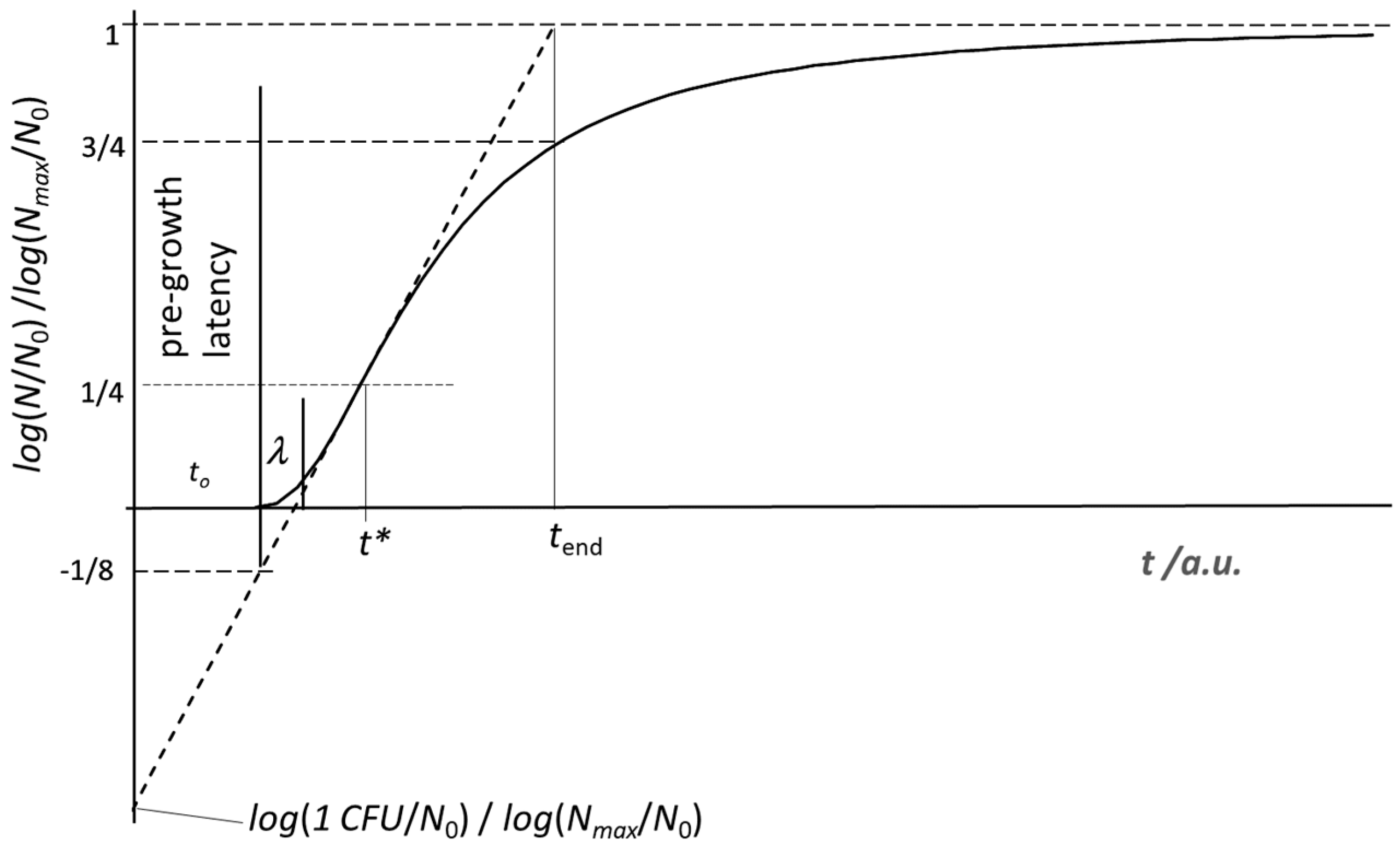
In spite of its substantially empirical and phenomenological nature, as its key parameters directly come from the experimental evidence, the model predicts some regularities of the growth trend that are common to every microbial species in any medium conditions (temperature, pH, water activity, favourable or adverse ingredients, etc.). Few examples can be of help. In the time lapse (t* − t0), the attained level of the population density, log2(N*/N0), is β/4. The straight line tangent to the growth curve at t = t* that corresponds to the maximum specific growth rate (namely, ) reaches the final growth level, log2(Nmax/N0), at t = tend. Furthermore, (tend − t0) = 3 (t* − t0) and log2(N/N0)tend = ¾β. The same straight line goes through the value log2(1 CFU/N0) at t = tstart that seems the best choice to set the origin of the time scale for the microbial culture [6]. This allows one to gather the growth curves of many different microbes, in different medium conditions, in a single master plot of reduced variables, , which does not depend on the log base used, and tR = (t − t0)/(t* − t0) [3,4,5]. Figure 1 reports the corresponding trend.
The phenomenological character of the proposed model does not provide any description of the cell behavior at the biochemical and physiological level but defines the collective character of the microbial population and its medium, which are supposed to affect each other and govern the overall destiny of the system [9]. For this reason, the function τ(t) does not reflect the behavior of the single cell, being a property of the whole system, namely the cells and hosting medium. This is in line with the evidence that the growth curve reflects the collective behavior of the microbial population within a changing medium.
After the rising trend of the growth phase, real microbial cultures tend to decay. In previous works [5,8,9] the pseudo exponential function
was proposed to describe the decay trend of microbial species that do not activate any physiological reaction to the adverse conditions responsible for the decline of N [8]. In the above expression, θ is the time from the start of the declining trend and d is an extra parameter defined through a best-fit routine of data relevant just to the decay trend. Equation (3) is a simple choice to meet the need for a reliable fit of the experimental data, but it has no specific connection with the behavior of the ideal planktonic culture for the growth trend.
N = Nmax exp(−θ2/d),
The present work aims to extend the model to the decay behavior of the ideal planktonic culture and provide a consistent expression for the decay trend.
2. Extension of the Model
2.1. Useful Tools for Predictive Microbiology Applications
The model implies a number of useful relationships, including the equation of the straight line tangent to the growth curve at t = t*, namely,
since (t* − t0) = (αβ/3)0.5.
As long as only the time differences appear, Equation (4) holds for any time origin. For the sake of simplicity, one may use the scale of the experimenter, namely, t = 0, at the start of the experiment. The straight line intercepts the time axis at t = t(0). Equation (1) states that:
Equation (5) is a very manageable predictive tool, as one can tentatively draw the straight line tangent to the growth trend and roughly estimate the values of t* and t(0) to approximately single out t0 on the time scale.
Equation (4) predicts this for t = t0, y = −β/8, which allows for the evaluation of β.
If θ is the time scale for the microbial culture, its origin occurs after some gap, tgap, from t = 0. Equation (4) keeps its structure, namely,
The suitable choice for the time origin for the microbial culture is that, for θ = 0, N = 1 CFU. This implies that, for t = tgap, namely, θ = 0, y = log2(1CFU/N0), as the variable of the y-axis is log2(N/N0). One can accordingly single out tgap on the time scale of the experimenter and replace the t values with θ values. Previous papers [8,9] suggested an interpretation of tgap.
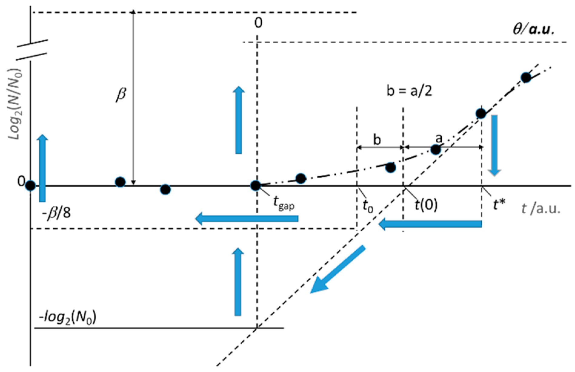
With the guideline of the above equations, few experimental data of the early trend of the growth progress allow a naked-eye estimation of tgap, t0, t*, and β, which can be very useful for a rough prediction of the expected growth of the microbial culture (Figure 2). Once more data become available, a best-fit routine can provide adjusted values of these parameters.
Equation (6) in powers becomes:
or
Equation (8) defines the maximum attainable level of the microbial population (in the given medium). Since the growth curve bends below the straight line described by Equation (6), such an Nmax value is actually larger than the real one. Nonetheless, Equation (7) states a correlation between Nmax and θ0. For a given N0, a large value of Nmax comes with a small value of θ0, and vice versa. The largest value of Nmax corresponds to θ0 = 0, namely,
Equation (9) defines a “theoretical” threshold that any microbial culture could not trespass.
2.2. Extension to the Steady and Decay Phases
The ideal planktonic culture remains the main character of the model: cell duplications are synchronic and no cell dies during the growth phase.
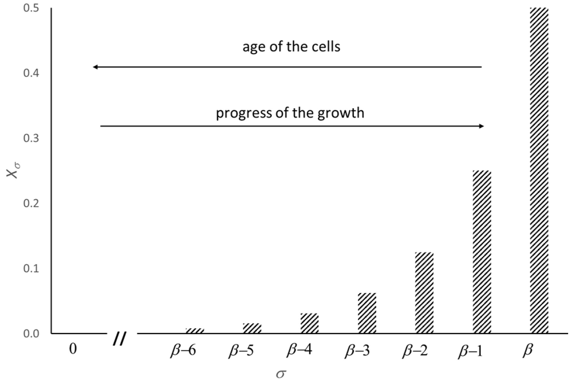
The starting N0 cells of the inoculum have the same age, but, during the growth phase, the microbial population acquires newborn cells. It is of help to recall that, throughout the growth phase, the youngest newborn cells account for 50% of the overall population, while the cells born in previous generation steps account for smaller fractions. The smaller the duplication step of the cell birth, σ, the smaller the population fraction, Xσ, related to the newborn daughter cells; the N0 cells represent a negligible fraction (Figure 3).
If t = ts is the threshold beyond which the rising trend of the growth curve ceases, the eventual population hosts cells of various ages. At t = ts, all the cells are still alive, but soon after the oldest ones start to die. Death would occur just because of the advanced cell age and the concomitant changes of the medium, including the exhaustion of the substrate.
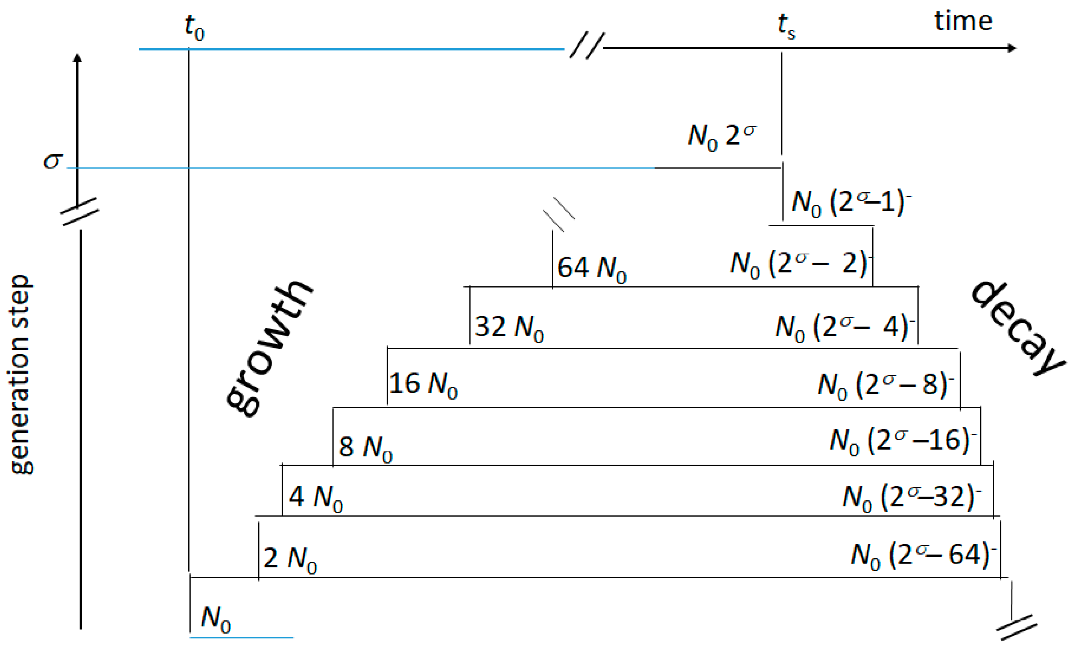
The first are the N0 cells of the inoculum, followed by those born in the first duplication step, followed by those born in the second duplication step, and so on. This means that, upon approaching the end of the decay phase, the eventual microbial population hosts cells of the same age, the number of which is half of the overall microbial population at t = ts.
In order to account for such generation scanning, the surviving population at t > ts should obey an expression like:
The pace of the decay, τd, must depend on the accompanying changes of the medium. It seems likely to suppose that the medium conditions worsen as time goes by (Figure 4).
A likely expression of τd can be:
The surviving population would therefore be:
Equation (12) is equivalent to Equation (3) that was already tested with a number of case studies [5,8,9], but is formally more consistent with the model used to describe the growth trend, as it explicitly accounts for the generation ranking. Equations (2) and (12), which define the growth and decay trend, respectively, imply the same value of (N/N0) for t = ts, no matter the value of the parameter, d.
It is worth noting that the so-called steady phase corresponds to the early decay of the ideal microbial population (Figure 5). The population level is not steady but decreases undetectably in log units.
The choice of the start of this phase, ts, is somewhat arbitrary, while its duration largely depends on the value of the parameter, d. The larger d, the flatter the pseudo steady trend. A large d reflects a slow decay of the older generations that are responsible for the early pseudo steady trend of the (N/N0) decay. A small d makes the early decay trend bend downward and form a broad maximum when matched with the rising growth trend, which does not attain any steady level [13] (see below). However, the arbitrary choice of ts has a limited impact on the early trend of growth that still obeys to Equation (2).
The use of a single function that encompasses the whole growth and decay (G and D) evolution of the system is of practical relevance to describe the effects of bactericidal or bacteriostatic drugs, injected at some point of the growth progress [9]. A simple choice can be:
For t = ts, Equation (13) yields practically the same value as Equation (2) only if (ts − t0)2 « δ. When the value of δ is not large enough, the function expressed by Equation (6) has a maximum (Figure 6) at:
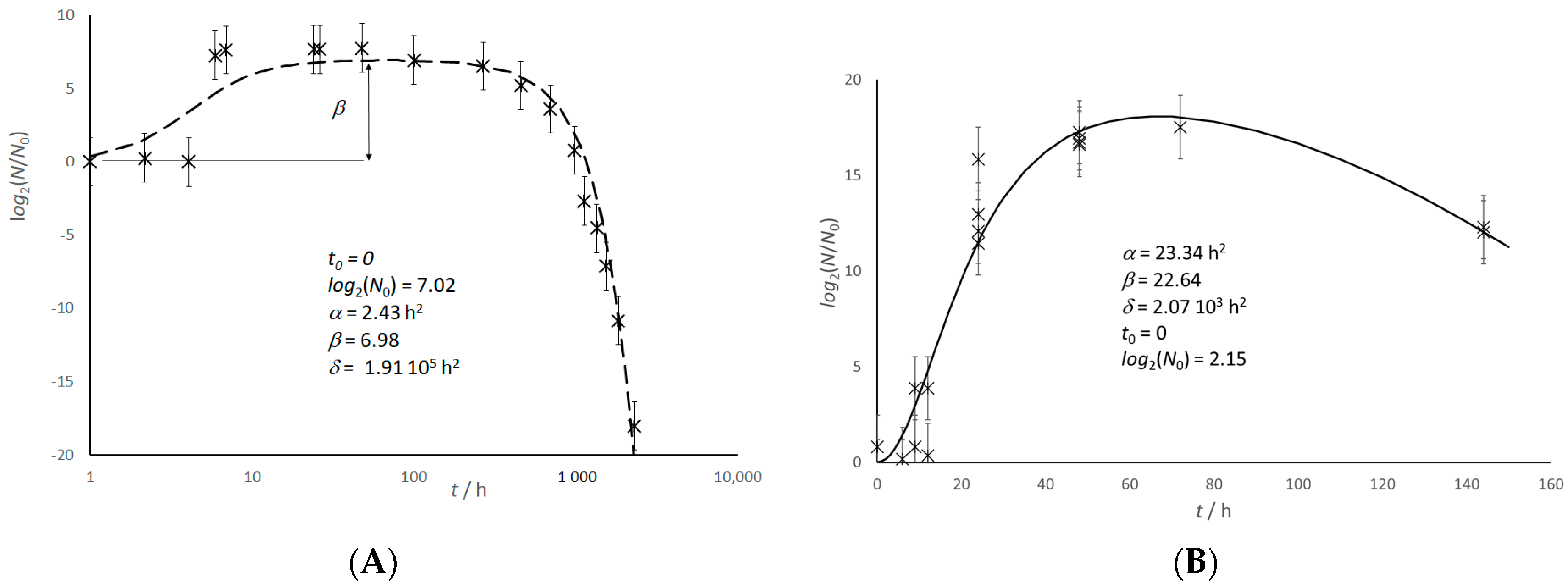
Figure 7 reports a couple of examples drawn from experimental data reported in the ComBase archive.
A single function for the whole evolution of a microbial culture comes also from a quasi-chemical approach [13], which nonetheless requires the definition and evaluation of a number of empirical parameters and still aims to reproduce the growth curve from the supposed behavior of the single cells. As mentioned above, this does not make sense in principle, as the growth curve reflects the collective behavior of the system, which includes cells and medium, and, therefore, is the result of many kinds of cell-cell and cell-medium interactions that are more than the parameters of any manageable kinetic model for the supposed behavior of the single cells. This means that the values of the parameters of such deterministic model actually have no physical or biological meaning.
The model of the ideal planktonic culture instead is phenomenological and does not pretend to gain any information, or start from any assumption, about the behavior of the single cells. Nonetheless, this model allows one to recognize that the pre-growth, growth, and steady phases are self-correlated events, which seem “planned” since the true start of the whole process at θ = 0. This time origin also comes from the fitting parameters (Figure 2) and does not necessarily coincide with the start of the experiment [8,9]. What makes the model appealing is that the approximate values of N0, t*, and the specific growth rate at t = t* (which come from the early steps of the growth trend) are sufficient to obtain the approximate values of the parameters α and β, as well as of the “true” zero of the time scale [8,9]. This makes the model a “predictive” tool for the growth trend. The estimation of the parameter d in Equation (5) or δ in Equation (6) requires few (i.e., no more than two or three) additional experimental data about the late evolution of the microbial culture (Figure 7), especially when one has to test specific adverse effects, such as those of injected bacteriostatic or bactericidal drugs [9].
3. Conclusions
The evolution of a microbial growth corresponds to the behavior of the whole system, namely, cells and medium. In the case of an ideal planktonic culture, such evolution looks like a planned event. The paper extends the model of an ideal planktonic culture [3,4,5,6,7,8,9] to some guidelines for predictive applications and to the decay trend. The formers make the model an efficient predictive tool allowing for a naked eye estimation of the parameters starting from few experimental data related to the early steps of the growth. These parameters do not concern the start and the duration of the intermediate pseudo steady phase, which actually corresponds to the early decay of the microbial population that occurs through consecutive steps. During this phase, the cells die following the generation rank (σ = 0, 1, 2, …) with a pace that becomes quicker upon approaching the final decline. The parameter d (or δ if a single function is used for the whole growth and decay evolution), which is responsible for the steepness of the decay trend, also determines the shape of the intermediate phase that can show a pseudo steady trend or a broad maximum between the rising and declining branch of the microbial population. The model is supported by a number of experimental evidence reported in previous papers [3,4,5,6,7,8,9].
Funding
This research received no external funding.
Data Availability Statement
Request all the data from the author.
Conflicts of Interest
The authors declare no conflict of interest.
References
- Cavagna, A.; Cimarelli, A.; Giardina, I.; Parisi, G.; Santagati, R.; Stefanini, F.; Viale, M. Scale-free correlations in starling flocks. Proc. Natl. Acad. Sci. USA 2010, 107, 11865–11870. [Google Scholar] [CrossRef] [PubMed] [Green Version]
- Ballerini, M.; Cabibbo, N.; Candelier, R.; Cavagna, A.; Cisbani, E.; Giardina, I.; Lecomte, V.; Orlandi, A.; Parisi, G.; Procaccini, A.; et al. Interaction ruling animal collective behavior depends on topological rather than metric distance: Evidence from a field study. Proc. Natl. Acad. Sci. USA 2008, 105, 1232–1237. [Google Scholar] [CrossRef] [PubMed] [Green Version]
- Schiraldi, A. Microbial growth in planktonic conditions. Cell Develop. Biol. 2017, 6, 185. [Google Scholar] [CrossRef] [Green Version]
- Schiraldi, A. A self-consistent approach to the lag phase of planktonic microbial cultures. Single Cell Biol. 2017, 6, 3. [Google Scholar]
- Schiraldi, A. Growth and decay of a planktonic microbial culture. Int. J. Microbiol. 2020, 2020, 4186468. [Google Scholar] [CrossRef] [PubMed]
- Schiraldi, A.; Foschino, R. An alternative model to infer the growth of psychrotrophic pathogenic bacteria. J. Appl. Microbiol. 2021, 1, 1–8. [Google Scholar] [CrossRef]
- Schiraldi, A.; Foschino, R. Time scale of the growth progress in bacterial cultures: A self-consistent choice. RAS Microbiol. Infect. Dis. 2021, 1, 1–8. [Google Scholar] [CrossRef]
- Schiraldi, A. Batch Microbial Cultures: A Model that can account for Environment Changes. Adv. Microbiol. 2021, 11, 630–645. [Google Scholar] [CrossRef]
- Schiraldi, A. The Origin of the Time Scale: A Crucial Issue for Predictive Microbiology. J. App. Env. Microbiol. 2022, 10, 35–42. [Google Scholar] [CrossRef]
- Baranyi, J. Comparison of Stochastic and Deterministic Concepts of Bacterial Lag. J. Theor. Biol. 1998, 192, 403–408. [Google Scholar] [CrossRef] [PubMed]
- Ahmer, B.M.M. Cell-to-cell signalling in Escherichia coli and Salmonella enterica. Mol. Microbiol. 2004, 52, 933–945. [Google Scholar] [CrossRef] [PubMed]
- Leiphart, R.J.; Chen, D.; Peredo, A.P.; Loneker, A.E.; Janmey, P.A. Mechanosensing at Cellular Interfaces. Langmuir 2019, 35, 7509–7519. [Google Scholar] [CrossRef] [PubMed]
- Doona, C.J.; Feeherry, F.E.; Ross, E.W. A quasi-chemical model for the growth and death of microorganisms in foods by non-thermal and high-pressure processing. Int. J. Food Microb. 2005, 100, 21–32. [Google Scholar] [CrossRef] [PubMed]
- Kocharunchitt, C.; Ross, T. Challenge Studies Involving Cheese Production; Food Safety Centre, University of Tasmania: Hobart, Australia, 2015. [Google Scholar]
- Salazar, J.K.; Bathija, V.M.; Carstens, C.K.; Narula, S.S.; Shazer, A.; Stewart, D.; Tortorello, M.L. Listeria monocytogenes growth kinetics in milkshakes made from naturally and artificially contaminated ice cream. Front. Microbiol. 2018, 9, 62. [Google Scholar] [CrossRef] [PubMed]
Figure 1.
The growth trend according to the present model. The reduced variable on the y-axis holds for any log base. The intercept of the straight line tangent (dotted line) to the growth curve at t = t* dictates the “true” (for the microbial culture) origin of the time scale (t = 0), which can be different from the start of the experiment. It is worth noticing the neat distinction between the pre-growth latency, t0, and the lag phase, λ, considered in most models reported in the literature [10].

Figure 2.
Preliminary steps for a naked eye prediction of the growth parameters. The arrows indicate the estimation steps, according to the guidelines reported in the text. The variable time is “t” or “θ” for the experimenter and the microbial culture, respectively. Dotted lines correspond to a naked eye estimation. The values of tgap, t0, t(0), t*, and β are tentative approximations. N0 has a known value. Full dots stand for experimental data.

Figure 3.
Population fraction, Xσ, of the newborn cells at the duplication step, 0 ≤ σ ≤ β (see text). The plot allows for the ranking of the microbial population according to the age of the cells.
Figure 3.
Population fraction, Xσ, of the newborn cells at the duplication step, 0 ≤ σ ≤ β (see text). The plot allows for the ranking of the microbial population according to the age of the cells.

Figure 4.
Sketched picture of the growth and decay of the ideal planktonic culture of the present model. At each step, 0 ≤ σ ≤ β (see text), the microbial population doubles (growth) or loses the oldest remaining generation (decay). The distance between steps depends on the variable duplication time (growth, Equation (1)), or shrinks (decay, Equation (4)) as the medium conditions worsen.

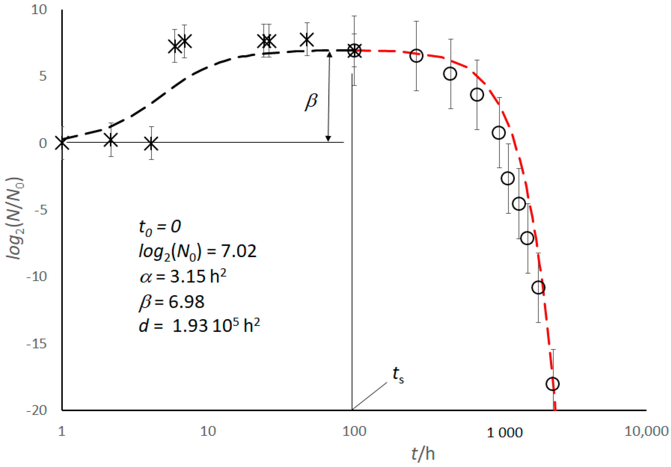
Figure 5.
E. coli culture in feta cheese. Growth (black dashed line) and Decay (red dashed line) trends according to Equations (2) and (12), respectively. The insert reports the corresponding parameters, which come from the best fit of experimental data, adjusted for the log base after [14]. Time is in a log10 scale. Bars correspond to the standard error.

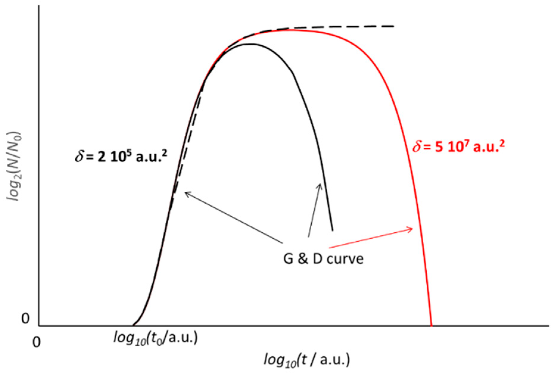
Figure 6.
A single function describes the whole growth and decay (G and D) evolution of the microbial culture. Trends according to Equation (6) with different values of the parameter δ. When the decay pace is quick (small δ, black line), a broad maximum of the G and D trend replaces the pseudo steady phase (large δ, red line). In any case, the early rising trend of the growth (dotted line) does not change. For the sake of comparison, the abscissa is in log10 scale.


Disclaimer/Publisher’s Note: The statements, opinions and data contained in all publications are solely those of the individual author(s) and contributor(s) and not of MDPI and/or the editor(s). MDPI and/or the editor(s) disclaim responsibility for any injury to people or property resulting from any ideas, methods, instructions or products referred to in the content. |
© 2023 by the author. Licensee MDPI, Basel, Switzerland. This article is an open access article distributed under the terms and conditions of the Creative Commons Attribution (CC BY) license (https://creativecommons.org/licenses/by/4.0/).
Share and Cite
MDPI and ACS Style
Schiraldi, A. The Growth Curve of Microbial Cultures: A Model for a Visionary Reappraisal. Appl. Microbiol. 2023, 3, 288-296. https://doi.org/10.3390/applmicrobiol3010020
AMA Style
Schiraldi A. The Growth Curve of Microbial Cultures: A Model for a Visionary Reappraisal. Applied Microbiology. 2023; 3(1):288-296. https://doi.org/10.3390/applmicrobiol3010020
Chicago/Turabian StyleSchiraldi, Alberto. 2023. "The Growth Curve of Microbial Cultures: A Model for a Visionary Reappraisal" Applied Microbiology 3, no. 1: 288-296. https://doi.org/10.3390/applmicrobiol3010020