Feedback Data Processing for Maintenance Optimization and Grouping—An Application to Road Markings

Abstract

In recent years, the maintenance of multicomponent systems has been discussed in many papers. The aim of these studies is to use the maintenance duration of one component for the maintenance of other components to minimize the total maintenance cost of the system. The complexity of the maintenance of this kind of system is due to its structure and its large number of components. The present paper suggests a grouped maintenance policy for multicomponent systems in a finite planning horizon based on the systemic inspection feedback data. The system considered is periodically inspected. Then, the collected data are triply censored (left, right, and interval censored). The proposed grouped maintenance strategy starts by clustering the components into g clusters according to their degradation model. Then, an expectation minimization algorithm is applied to correct the censorship in the data and to associate a Weibull distribution with each cluster. The proposed grouped maintenance strategy begins by specifying an individual maintenance plan for each cluster by identifying an optimal replacement path. Then, this step is followed by finding an optimal grouping strategy using a genetic algorithm. The aim is to identify a point in time when the components can be maintained simultaneously. To illustrate the proposed strategy, the grouped maintenance policy is applied to the feedback data of the road markings of French National Road 4 (NR4) connecting Paris and Strasbourg.

1. Introduction

The development of maintenance strategies for multicomponent systems is an increasingly important topic in the field of reliability. In the industrial field, choices must be made between different maintenance options such as those regarding the nature of the maintenance (preventive or corrective) and the frequency or type of maintenance action to perform. When a single-component system is considered, maintenance optimization seems “simple” (the optimization is then a strategy of finding the best times to intervene while accounting for the dynamics of system degradation and constraints relating to availability, safety, maintainability, etc.), but the problem increases in complexity as the size of the system increases. Complexity is added when there are interactions (economic, stochastic, etc.) between the components of the system. In this case, the optimal solution for a multicomponent system can be very far from a “stacking” of the individual optimal strategies characterizing each component considered alone. Research on maintenance optimization dates to the 1960s, and many works try to deal with some aspects of this particularly hard and complex problem: from modeling the degradation processes to taking on constraints such as reliability, staff availability, costs, etc., or more recently, taking advantage of the advancements in monitoring or new technologies such as artificial intelligence, machine learning, big data, and the Internet of Things. For more details, readers could refer to the last literature review on maintenance optimization proposed by Pincirolli et al. [1].

To optimize the maintenance cost of a multicomponent system, approaches that group maintenance actions are generally proposed. These groupings are beneficial from an economic perspective (in particular, grouping reduces fixed costs), but also ensure that the system functions well overall. In recent years, many maintenance strategies have been proposed that bundle maintenance tasks. Several papers have discussed this problem; see, for example, Refs. [2,3,4,5]. The aim of these strategies is to minimize maintenance costs and ensure system availability. For example, Dekker et al. reviewed the literature on multicomponent system maintenance strategies considering the economic dependence between systems’ components [2]. They listed different types of strategies: stationary politics with a long-term stable situation and dynamic strategies that account for the modification of the system in the short term. Those strategies handle either corrective or preventive maintenance or, in some cases, combined corrective and preventive maintenance actions. The operational nature of the system indicates the type of planning horizon. In [5], most grouping policies are concerned with series systems because the shutdown of one component leads to the total shutdown of the system. Then, authors proposed a maintenance strategy for multicomponent systems with dynamic contexts and a finite horizon model to optimize online the maintenance strategy in dynamic contexts. The paper neglects the maintenance duration and the impacts of the grouped maintenance on the production systems. The proposed strategy was applied to a numerical example of a 16-component system. The results highlight the preference and robustness of the proposed maintenance grouping strategy.

Proposing a maintenance grouping strategy for a system with several components starts with the proposal of an individual preventive maintenance plan for each component. In industry, preventive maintenance is the act of periodically performing a maintenance action to fix or replace a component before its failure. Different preventive maintenance approaches exist. A systematic approach identifies an optimal maintenance path in accordance with the lifetime of the component and the maintenance cost; see, for example, [6]. The aim of a conditional policy is to determine an optimal preventive degradation threshold according to the degradation model, maximum degradation threshold, and maintenance cost [7]. The last preventive maintenance type is the predictive approach. This approach is like the conditional approach, but the preventive threshold is replaced by a failure risk as the remaining useful life [8]. This paper considers the systematic approach.

To evaluate the state of a system S at time t, a decision variable is assigned for each component to identify whether it has failed or is operating, and since the maintenance strategy proposed in this paper is based on reliability, it is necessary to identify the state space of the system. In our study, the decision variables are therefore the ones that provide the renewal (or repair) times. In the literature, two approaches have generally been considered. The state space D_ℶ of a given component denoted i can be either continuous (e.g., the percentage of pavement cracked) or discrete with a finite number of states. In this study, the states can be reduced to two: respectively, the operating and failure states.

In the case in which the decision variable is continuous, a component is considered to have failed if this variable exceeds a set failure threshold. In this work, the condition of each component i is periodically inspected (an inspection step is set), and the decision variable is continuous. With this approach, the exact date when the component crosses the failure threshold is not known. Then, the inspection data are said to be censored. The censored data are categorized into three types: left censored, interval censored, and right censored. Thus, to address this kind of problem, the literature proposes three families of algorithms: expectation–maximization (EM) [9,10], stochastic expectation–maximization (SEM) [11,12], and Bayesian restoration maximization (BRM) [13,14,15]. In this work, an EM algorithm is considered.

Although there are several papers in the literature that study the maintenance of road infrastructure, no studies take into consideration all the components of the road infrastructure (pavement and marker lines). The main goal of this paper is, therefore, to propose an optimal maintenance plan of all the marker lines of a given road infrastructure regarding a grouping approach. To achieve this goal, a specific data processing and analysis approach is proposed. This study is motivated by the needs of autonomous and connected vehicles for road infrastructure.

2. Introduction to the Problem and the Use Case

Preventive maintenance has been discussed by many authors. In industry, preventive maintenance is the act of periodically performing a maintenance action to x or replace a component before its failure. In the literature, many preventive maintenance strategies exist. In [16], two types of preventive maintenance policies are considered. The first is useful for maintaining simple equipment, and the second is useful for maintaining complex systems. In the same context, Valdez-Flores et al. included optimization models for the repair, replacement, and inspection of systems subject to stochastic deterioration [17]. In 2002, Wang proposed different types of preventive maintenance: the age replacement policy, random age replacement policy, block replacement policy, and repair cost limit policy [18]. Finally, Barlo and Proshan concluded that the age replacement policy is an economical way to determine block replacement age [19]. Under this policy, a component is replaced at age T* or after failure. Refs. [20,21] introduced another type of preventive maintenance policy (imperfect maintenance) with minimal repair. This policy is equivalent to a perfect repair with probability p and a minimal repair with probability 1 − p. After imperfect maintenance, the component is not as good as new but is younger. In the same context, Ref. [22] discussed conditional preventive maintenance. This type of policy is based on controls and inspections to guarantee the optimal availability of a component. This paper considered an age replacement policy.

Then, the optimization of maintenance strategies is also a key issue. As many papers can easily be found in the literature, we chose to focus on works dedicated to road infrastructure. Thus, Guan et al. proposed a multi-objective optimization model considering the interactions between pavement condition and traffic dynamics for the planning of multi-year road network maintenance considering a genetic algorithm [23]. In [24], authors proposed a multiple Markov decision process model and a priority-based two-stage method for determining optimal maintenance decisions for road infrastructure. In [25], based on a semi-Markov approach to model the road deterioration through a Weibull model, linear programing models were proposed to define optimal maintenance policies to minimize the lifecycle cost of a road.

As mentioned in Section 1, our work focuses on multicomponent systems that refer to a mixture of a few components which may interact with each other. These components are structured in different configurations: serial, parallel, or a complex combination of serial and parallel structures. The structure of the system represents the way in which the components are arranged to perform a common function. The modeling of the system structure is vital because it conditions the overall functioning of the system. A serial system works if all its components work, but a parallel system works if at least one of its components works.

In industry, grouping maintenance is a way to minimize preventive maintenance costs. The aim of the method is to identify the optimal time to simultaneously maintain a complex system’s components. According to [2], the dependencies between the system’s components are classified into stochastic, structural, and economic. Many grouped maintenance policies are presented, and most consider only economic dependence.

Nguyen introduced two types of grouped maintenance policies: dynamic policies that allow maintenance plans to be updated in a dynamic context and stationary policies that do not consider the dynamic context [26]. However, grouping maintenance actions can also be conducted in a dynamic context [4,5]. In this case, some changes both in the costs during the planning horizon and in the system’s structure must be introduced. Ref. [27] proposed a stationary grouped maintenance strategy for systems with complex structures. The grouping methodology is presented as a policy for making the maintenance cost cheaper than separately performing the maintenance activities. In the same context, [3] proposed a grouped maintenance optimization for series systems subject to reliability constraints. Most of the grouping strategies are based on genetic algorithms, and some recent papers explored other operational research solutions. Thus, a particle swarm optimization algorithm was proposed for both optimizing the availability of a system and minimizing the cost of its preventive maintenance through a grouping strategy [28]. More recently, a clustering approach was proposed for optimal grouping maintenance strategies for complex structure systems [29]. Finally, some grouping strategies tried to take constraints into account. Up to now, only one constraint is generally introduced in grouping policies, mainly connected to maintenance teams. Thus, Do et al. proposed a dynamic maintenance grouping strategy, optimized on a rolling horizon using a genetic algorithm, under both availability and limited repairmen constraints [30]. In a road context, Jha et al. considered a cost minimization problem considering work shift and overtime constraints. An algorithm using Floyd’s shortest path method was developed to optimize the time and paths for efficient inspection of highway assets [31].

In our paper, the proposed methodology considers the interdependence existing between components. In conclusion, the main aim of this study is to propose a grouped maintenance policy for multicomponent systems in a finite planning horizon.

For some systems, the components do not really fail but reach a serviceability threshold. Therefore, even for serial systems, if a component reaches a serviceability limit state, the entire system remains in operation. Thus, it is important to inspect the system to know the condition of each component. As introduced in Section 1, the aim of this paper is to determine an optimal maintenance strategy for road marking considering a grouping approach. For this, a specific data processing approach to analyze the feedback data of multicomponent systems is defined and introduced. 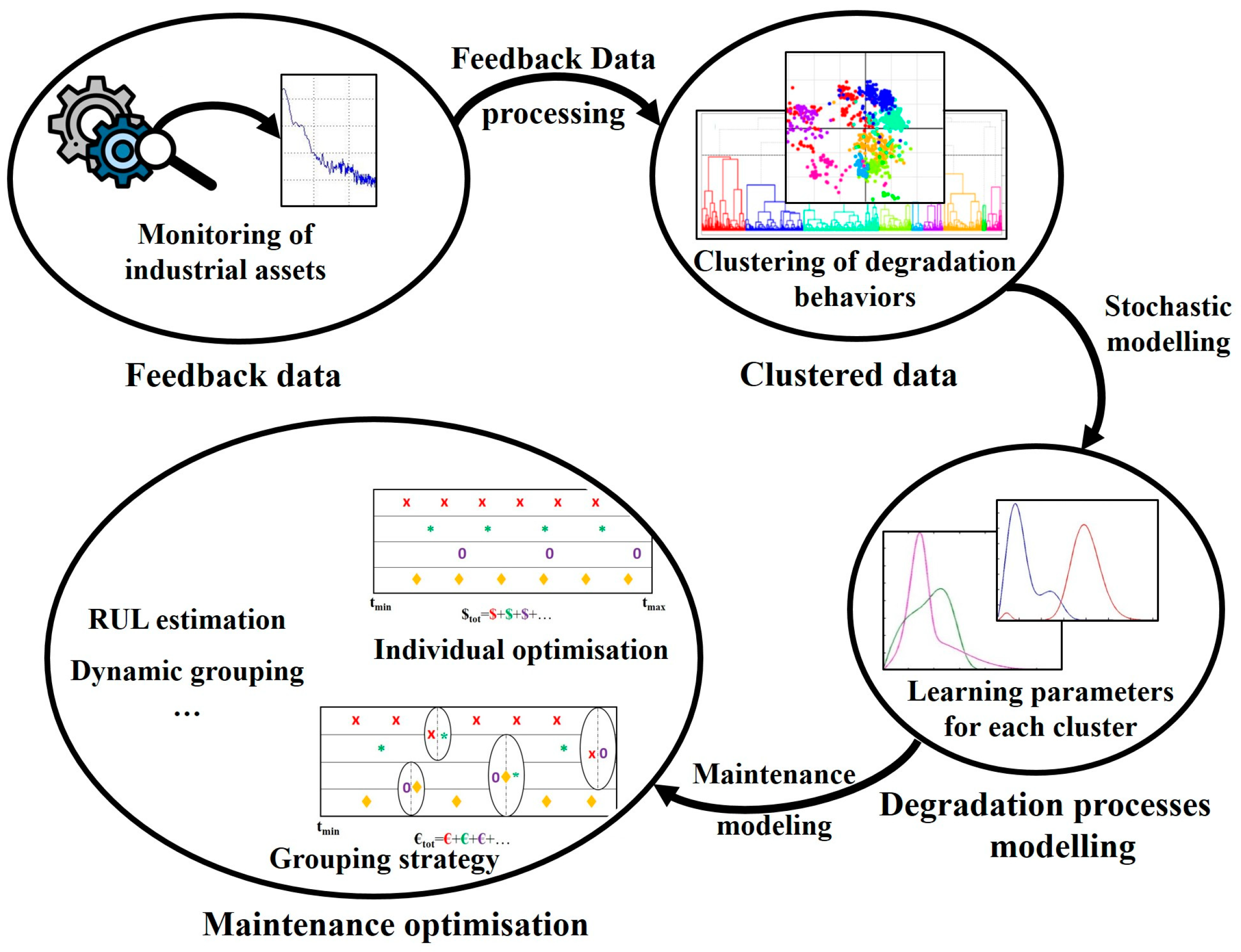The contribution of this study is summarized in Figure 1, which introduces our contribution and all the algorithms used. As illustrated in Figure 1, the proposed grouping strategy involves four main steps:

• Data collection and analysis;
• Classification of system components into several clusters according to their degradation process;
• Individual maintenance optimization for each cluster;
• Maintenance action grouping, considering the interactions between the system components.

The contributions of this paper focus on the last three steps previously introduced. Each of these steps will be discussed and detailed in the next sections.

The proposed strategy is applied to periodically inspected feedback data. The exact failure time is not generally observed, and the feedback data contain multiple types of censoring: left censoring, interval censoring, and right censoring. To address this kind of data, a Weibull analysis is proposed for estimating the failure time using maximum likelihood estimation (MLE).

In 2007, Hunter suggested using the EM algorithm to estimate the date of failure [8]. In the case of incomplete or missing data, an EM algorithm is a useful method for finding the maximum likelihood. A Weibull analysis is a commonly used methodology for performing life data analysis. Indeed, it is an effective method for determining reliability characteristics and has demonstrated a good “agility” to fit the behavior of a population. Ducros and Pamphile proposed EM, SEM, and BRM algorithms for estimating the Weibull parameters [14]. In the second section of this paper, an extension of the EM algorithm for processing left- and right-censored data is presented. The proposed algorithm is applicable to all observation vectors independent of the nature of the censoring.

In this paper, the EM algorithm proposed by M. Redondin is used. According to the work of Sathyanarayanan, this algorithm is suitable for the simulation of road marking degradation [32]. To simplify the study, the components of the system are clustered into groups according to their degradation level. Then, a maintenance strategy is proposed for each cluster.

In data mining, two types of classification exist: supervised and unsupervised. Supervised classification is the data mining algorithm most often used for quantitative analysis. In the literature, supervised classification algorithms are often used with image data. In this case study, agglomerative hierarchical clustering (AHC) combined with a factor analysis of mixed data (FAMD) is considered since its use has been proven relevant for road markings [33]. This strategy is introduced in Section 4.

In this article, the feedback data (the inspection date t and the level of degradation of a component) are classified in a state space marked D. In this framework, the data are censored, so the state space is divided into four subspaces according to the nature of the censoring. D = D_E ∪ D_L ∪ D_I ∪ D_R, where D_E represents the exact data, D_L the left-censored data, D_I the interval-censored, data and D_R the right-censored data. Then, the data collected during inspections are clustered into k clusters according to their degradation model. To correct the censoring of each cluster C_j with j ∈ {1, …, k}, an EM algorithm is applied to estimate the exact dates of failure and assign a probability distribution for the degradation model for each cluster C_j with j ∈ {1, …, k}. Once the parameters of the Weibull distribution (α_j, β_j) are estimated and the various maintenance costs are set, an optimal replacement period T_j^∗ is defined for each cluster C_j. For minimizing maintenance costs, a bundling strategy is applied to identify a maintenance date that bundles several maintenance actions together.

This paper considers an example structured as a series system whose components are independent and periodically inspected. The decision variable is continuous.

In conclusion, although the case study is limited to serial systems, the minimum requirement to apply this grouping strategy is to have an inspection history of the different components of the system. The feedback data process and grouped maintenance strategy, illustrated in Figure 1, is proposed for:

• Complex structure systems;
• Finite-horizon planning;
• Age-based replacement policy.

This paper is structured as follows. In Section 3, a strategic clustering of the system components is discussed. The aim is to group the components that degrade in the same way in order to assign a maintenance strategy to each cluster. The feedback data considered in this paper are censored. Instead of correcting the censoring for each component, it is corrected for each cluster by applying an EM algorithm, presented in Section 4. The maintenance policy chosen (for each cluster) in this paper is an age-based policy. It is discussed in detail in Section 5. To minimize the preventive maintenance cost of a given system, a grouping policy is proposed in Section 6, and its application is discussed in Section 7.

3. Strategic Clustering for Preventive Maintenance

To simplify the study, all components of a given system S are clustered into g groups according to their degradation level, observed between two inspections I_t and I_t+1. The aim of this strategy is to identify the internal grouping in a set of data to apply a Weibull analysis and propose a preventive maintenance strategy adapted to each cluster C_j. In the absence of a class label, the clustering method used is unsupervised. In data mining, there are numerous unsupervised clustering algorithms, such as k-means, hierarchical clustering, and Gaussian mixture models. In [33], authors suggested clustering the components using an AHC. Each group C_j contains those components that degrade in the same way. An automatic classification and analysis of multiple-criteria decision making was proposed in [34]. The unsupervised clustering algorithms are used to generate rules from a learning database. In both papers, [33,34], the AHC is used because it offers a simple and clear approach to facilitate the structuring of information. It returns a hierarchical structure that is more informative than the unstructured set of clusters produced by k-means, for example.

According to [30], hierarchical clustering is an approach that builds hierarchies of clusters through two approaches:

• Agglomerative: A bottom-up strategy, where each observation starts in its own cluster, and pairs of clusters are merged upwards in the hierarchy;
• Divisive: A top-down strategy, where all the observations start out in the same cluster, and then the clusters are divided recursively downwards in the hierarchy.

To identify which clusters to merge or split, a measure of the distance between clusters is introduced. Ref. [33] proposed the Ward distance that defines the distance between two clusters, C_j and C_j′, as the sum of squares, which increase when they are merged. This parameter is given by (1), where $d$ is the Euclidean distance.

$$d_w\left(C_j,C_{j^{\prime }}\right)=\frac{\mathrm{d}(m_j,m_{j^{\prime }})}{\frac{1}{n_j}+\frac{1}{n_{j^{\prime }}}}$$

(1)

where m_j and m_j′ are the average profiles of the clusters, n_j and n_j, are the corresponding numbers of observations in each cluster, and d is the Euclidian distance.

Then, Tidjani et al. chose the optimal number of clusters based on the semi-partial R² criterion [32]. This term represents the loss between inertial class references. Hierarchical clustering is a method that builds a cluster tree (named dendrogram) to present the data. A node in the dendrogram contains a group of similar data.

As mentioned in the previous section, the data considered in this work are censored. To correct the censored data, a Weibull analysis is applied to each cluster C_j. The goal of the analysis is to estimate the exact failure date and the associated parameters of the Weibull distribution. This methodology is presented in the next section.

4. EM Algorithm

The Weibull distribution considered in this paper is defined by the probability density function given in Equation (2), where α > 0 and β > 0 are the associated scale and shape parameters:

$$f\left(x\right)=\left\{\begin{array}{c}\frac{\beta }{\alpha }{\left(\frac{x}{\alpha }\right)}^{\beta -1}{e}^{-{\left(\frac{x}{\alpha }\right)}^{\beta }}ifx>0\\ 0 \hspace{1em} \hspace{1em}ifx\le 0\end{array}\right.$$

(2)

Assume that $W$ is the lifetime variable of the road markings. The observed data (τ₁, τ₂, …, τ_n) should be independent and identically distributed. The feedback data are censored. In this paper, three types of censored data are assumed:

• If failure occurs before the first inspection I₁, the data are left censored;
• If failure occurs between two inspections, the data are interval censored. The time interval in this case is [l, r], where l is the date of inspection I_l and r is the date of the l + 1 inspection;
• If failure has not been observed by the last observation, the data are right censored.

For simplicity, the censoring types are coded as follows:

i = 1, …, n

$$\forall \mathrm{i}=1,\dots ,\mathrm{n},{\mathsf{\delta }}_i=\left\{\begin{array}{c}0 if {\tau }_i is uncensored\\ 1 if {\tau }_i is left censored\\ 2 if {\tau }_i is interval censored\\ 3 if {\tau }_i is right censored\end{array}\right.$$

(3)

The observed data are divided according to the censoring type:

$${\mathrm{D}}_E=\left\{\tau \in \left(\left({\tau }_1,{\delta }_1\right),\dots ,\left({\tau }_n,{\delta }_n\right)/{\mathsf{\delta }}_i=0\right)\right\}$$

(4)

$${\mathrm{D}}_L=\left\{\tau \in \left(\left({\tau }_1,{\delta }_1\right),\dots ,\left({\tau }_n,{\delta }_n\right)/{\mathsf{\delta }}_i=1\right)\right\}$$

(5)

$${\mathrm{D}}_I=\left\{\tau \in \left(\left({\tau }_1,{\delta }_1\right),\dots ,\left({\tau }_n,{\delta }_n\right)/{\mathsf{\delta }}_i=2\right)\right\}$$

(6)

$${\mathrm{D}}_R=\left\{\tau \in \left(\left({\tau }_1,{\delta }_1\right),\dots ,\left({\tau }_n,{\delta }_n\right)/{\mathsf{\delta }}_i=3\right)\right\}$$

(7)

In statistics, MLE is a method for estimating the parameters of a distribution function. The uncensored data are computed as follows:

$$L\left(\alpha ,\beta \right)=\prod _{i=1}^{n}f\left({\tau }_i\right)$$

(8)

For censored data, the likelihood function is defined as:

$$L\left(\alpha ,\beta \right)={\prod }_{\tau \in D_E}^{}{f}_E\left(\tau \right){\prod }_{\tau \in D_L}^{}{F}_L\left(\tau \right){\prod }_{\tau \in D_I}^{}\left(R_I\left(l\right)-R_I\left(r\right)\right){\prod }_{\tau \in D_R}^{}{R}_R\left(\tau \right)$$

(9)

f_E is the probability density function of subspace D_E, and F_L(τ) = P ($𝒲$ < τ) is the cumulative distribution function of subspace D_L. This expression represents the probability that failure occurs before time τ, and R_L(τ) = 1 − F_L(τ) and R_R(τ) = 1 − F_R(τ) of subspaces D_I and D_R, respectively, represent the probabilities that failure will occur after τ.

In the case of censored data, the classical method is not applicable. In 2019, Redondin et al. proposed an extension of the EM algorithm for censored data [9]. This process interprets the censored data as missing data and iteratively computes two steps:

• The expectation step estimates the censored data according to a given Weibull distribution Ω(α, β);
• The maximization step estimates a Weibull distribution by MLE according to both the uncensored and complete data.

4.1. Expected Step

To simplify the EM algorithm, substituting $\alpha \leftarrow {\alpha }^{\frac{1}{\beta }}$ was suggested [35]. Following this modification, the Weibull density function is:

$$f\left(x\right)=\left\{\begin{array}{c}\alpha \beta {\left(x\right)}^{\beta -1}{e}^{-{\alpha x}^{\beta }}ifx>0\\ 0 \hspace{1em} \hspace{1em}ifx\le 0\end{array}\right.$$

(10)

In this step, the likelihood estimated is computed as the maximized expectation of the likelihood function conditional on the uncensored data.

$$L_C\left(\alpha ,\beta \right)=E\left[L\left(\alpha ,\beta \right)|\tau \right]$$

(11)

The aim of this strategy is to estimate the censored data; each one is a conditional expectation adapted for a specific censoring. The following estimators were proposed in [9]:

$$\widehat{t_L}=E\left[W|W<\tau \right]=\frac{\alpha \beta {\int }_0^{\tau }{x}^{\beta }{e}^{-{\alpha x}^{\beta }}dx}{1-e^{-{\alpha \tau }^{\beta }}}$$

(12)

$$\widehat{t_I}=E\left[W|l<W<r\right]=\frac{\alpha \beta {\int }_l^r{x}^{\beta }{e}^{-{\alpha x}^{\beta }}dx}{e^{-{\alpha l}^{\beta }}-e^{-{\alpha r}^{\beta }}}$$

(13)

$$\widehat{t_R}=E\left[W|W>\tau \right]=\frac{\alpha \beta {\int }_{\tau }^{+\infty }{x}^{\beta }{e}^{-{\alpha x}^{\beta }}dx}{-e^{-{\alpha \tau }^{\beta }}}$$

(14)

Using these estimators, the likelihood function L_c associated with the censored data in the estimation of the Weibull distribution parameters is defined by (15).

$$L_C\left(\alpha ,\beta \right)={\prod }_{t\in D_E}^{}{f}_E\left(t\right){\prod }_{\widehat{t_L}\in D_L}^{}{F}_L\left(\widehat{\widehat{t_L}}\right){\prod }_{\widehat{t_I}\in D_I}^{}{F}_I\left(\widehat{t_I}\right){\prod }_{\widehat{t_R}\in D_R}^{}{F}_R\left(\widehat{t_R}\right)$$

(15)

4.2. Maximization Step

The parameters of the Weibull density (α, β) annul the two partial derivatives of the completed log likelihood function.

$${\delta }_{\alpha }{L}_C=\frac{n}{\alpha }-{\sum }_{t\in D_E}{t}^{\beta }-{\sum }_{\widehat{t_L}\in D_L}{\widehat{t_L}}^{\beta }-{\sum }_{\widehat{t_I}\in D_I}{\widehat{t_I}}^{\beta }-{\sum }_{\widehat{R}\in D_R}{\widehat{t_R}}^{\beta }$$

(16)

$$\begin{gathered} {\delta }_{\beta }{L}_C=\frac{n}{\beta }-{\sum }_{t\in D_E}\ln \left(t\right)-{\sum }_{\widehat{t_L}\in D_L}\ln \left(\widehat{t_L}\right)-{\sum }_{\widehat{t_I}\in D_I}\ln \left(\widehat{t_I}\right)-{\sum }_{\widehat{t_R}\in D_R}\ln \left(\widehat{t_R}\right)- \\ \alpha \left[{\sum }_{t\in D_E}\ln \left(t\right)+{\sum }_{\widehat{t_L}\in D_L}{\widehat{t_L}}^{\beta }\ln \left(\widehat{t_L}\right)+{\sum }_{\widehat{t_I}\in D_I}{\widehat{t_I}}^{\beta }\ln \left(\widehat{t_I}\right)-{\sum }_{\widehat{t_R}\in D_R}{\widehat{t_R}}^{\beta }\ln \left(\widehat{t_R}\right)\right] \end{gathered}$$

(17)

In [9], authors proposed estimating the Weibull parameters (α, β) as a nonlinear problem. This problem is solved by a fixed-point approach. α is estimated by equation ∂_αL_c (α, β) = 0 as:

$$\alpha =\frac{n}{\sum _{t\in D_E}{t}^{\beta }-\sum _{\widehat{t_L}\in D_L}{\widehat{t_L}}^{\beta }-\sum _{\widehat{t_I}\in D_I}{\widehat{t_I}}^{\beta }-\sum _{\widehat{t_R}\in D_R}{\widehat{t_R}}^{\beta }}$$

(18)

The estimation of α clearly depends on β since Equation (18) is a function of β. Replacing α by (18) in (17), a function g(β), as ∂_βL_c = g(β) − β, is extracted in Equation (19). β is defined as the convergence point of the sequence in (20).

$$g(\beta )=\frac{1}{\frac{\sum _{t\in D_E}{t}^{\beta }\ln \left(t\right)+\sum _{s\in S}{\widehat{s}}^{\beta }\ln \left(\widehat{s}\right)}{\sum _{t\in D_E}{t}^{\beta }+\sum _{s\in S}{\widehat{s}}^{\beta }}+\frac{\sum _{t\in D_E}\ln \left(t\right)+\sum _{s\in S}\ln \left(\widehat{s}\right)}{n}}$$

(19)

where S is the set of lifetime durations corrected by the proposed EM algorithm over D_L, D_I, and D_R.

The fixed point of g(β) is β, where g(β) = β. Given the initial value, the problem is modeled as:

$${\left(U_n\right)}_{n\ge 0}=\left\{\begin{array}{c}{u}_0>0\hspace{1em}\hspace{1em}\hspace{1em}arbitrary\\ u_n=g\left(u_{n-1}\right)\hspace{1em}\hspace{1em}n>0\end{array}\right.$$

(20)

4.3. Iteration and Convergence

Given the arbitrary initial distribution Ω(α₀, β₀), Redondin et al. proposed that α₀ and β₀ are the MLE estimations when the censored data are ignored [10]. For each iteration k, the Weibull distribution is given by Ω(α_k, β_k). Using (20), β_k is computed as (21):

$${\left({\beta }_k\right)}_{k\ge 0}=\left\{\begin{array}{c}{\beta }_0>0\\ \alpha =\underset{x\to 0}{\lim }\left\{\begin{array}{c}{u}_0={\beta }_{k-1}\\ u_n=g\left(u_{n-1}\right)\end{array}\right.\end{array}\right.$$

(21)

Referring to [9], it was proposed to stop the iterations when |β_k − β_k−1| < 10⁻⁴. The EM algorithm convergence is defined by the convergence of the sequences (β_k)_k≥0 and (18):

$$\left\{\begin{array}{c}\beta =\underset{k\to \infty }{\lim }{\beta }_k\\ \alpha =\frac{n}{\sum _{t\in D_E}{t}^{\beta }+\sum _{\widehat{t_L}\in D_L}{\widehat{t_L}}^{\beta }+\sum _{\widehat{t_I}\in D_I}{\widehat{t_I}}^{\beta }+\sum _{\widehat{t_R}\in D_R}{\widehat{t_R}}^{\beta }}\end{array}\right.$$

(22)

Finally, the modification $\alpha \leftarrow \raisebox{1ex}{$1$}\!\left/ \!\raisebox{-1ex}{$\sqrt[\beta ]{\alpha }$}\right.$ is intended to return to Weibull distribution (2). When the associated Weibull parameters are defined, a preventive maintenance strategy adapted to each cluster can be proposed as introduced in the following section.

5. Individual Maintenance Strategy Optimization

The components of the system are clustered into g groups. For each cluster C_j (with j ∈ {1, g}), a Weibull analysis using the EM algorithm presented in the previous section is applied to identify the parameters (α_j, β_j). The policy suggested in this section is an age-based replacement for each cluster C_j. As illustrated in Figure 2, the preventive replacement of cluster C_j is carried out once the age of the component reaches a critical operational age T_j∗ (T_j∗ being the optimal replacement age of all components in cluster j). If the component fails between two replacement dates, the component is replaced, and the maintenance action cost is C_cj. To avoid over-maintenance, the age of the component is initialized at 0 after a corrective action and the preventive action scheduling is translated from the date of the failure.

The replacement of the component restores the system operating conditions to “as good as new”. The optimal age for replacing the components of cluster C_j is defined by (23), and T_j∗ presents the optimal frequency of preventive maintenance action.

$$T_J^{*}=\left\{T/C_{sys}\left(T\right)={min}_{t>0}\left(C_{sys}\left(t\right)\right)\right\}$$

(23)

The long-term asymptotic cost C(∞) defines the cost of the corrective maintenance per unit of time. This term is computed by (26). C(∞) depends on the mean time before replacement (MTBR). The MTBR is associated with the Weibull density Ω(α_j, β_j) of the jth cluster.

$$C\left(\infty \right)=\underset{t\to \infty }{\lim }{C}_{sys}\left(t\right)=\frac{C_p^j+C_c^j}{{\int }_0^{+\infty }{R}_j\left(x\right)dx}$$

(24)

$$C\left(\infty \right)=\underset{t\to \infty }{\lim }{C}_{sys}\left(t\right)=\frac{C_p^j+C_c^j}{MTBR}$$

(25)

$$C\left(\infty \right)=\underset{t\to \infty }{\lim }{C}_{sys}\left(t\right)=\frac{C_p^j+C_c^j}{{\alpha }_j\mathsf{\Gamma }\left(1+\raisebox{1ex}{$1$}\!\left/ \!\raisebox{-1ex}{${\beta }_j$}\right.\right)}$$

(26)

where $C_p^j$ and $C_c^j$ are, respectively, the cost of a preventive or corrective maintenance action for the jth cluster. To identify the benefit profit of preventive maintenance, the ratio $\frac{C_{sys}\left(t\right)}{C(\infty )}$ is used.

It measures the financial benefit of preventive maintenance at time t compared to corrective maintenance. The value of this ratio determines whether corrective maintenance or preventive maintenance is better. If it is over 1, corrective maintenance is more economically beneficial. In the opposite case, preventive maintenance provides more economical benefits.

The proposed maintenance strategy is applied to each cluster to identify an optimal path of maintenance. The next section presents a grouped maintenance strategy to minimize the maintenance costs.

6. Grouping Maintenance Strategy

As mentioned above, grouping maintenance actions can reduce the system maintenance cost. In this section, based on the formalism proposed in [5,31], a statistical grouped maintenance strategy is proposed. As presented in Section 1, this strategy is characterized by a finite planning horizon, denoted HZ, which will be defined in the next section.

6.1. Defining the Planning Horizon

The first step in defining the planning horizon is to determine the beginning date T_begin. In this case study, we will assume that T_begin = 0. To ensure that all the components are maintained, the end of the planning horizon, denoted T_end, is defined as:

$$T_{end}^{}={\mathrm{m}\mathrm{a}\mathrm{x}}_{i=1\dots N}\left\{t_{i^1}\right\}$$

(27)

where $t_{i^1}$ defines the first maintenance action for component i. To illustrate this method, an example is presented in Figure 3. In this example, HZ = HZ = [0, $t_{i^1}$]. In this planning horizon, components 1 and 2 are maintained twice and component N is maintained only once.

6.2. Mathematical Formulation of Economic Profit

For the problem of optimizing maintenance strategy for a multicomponent system by grouping maintenance actions, a candidate solution is presented as an array denoted Z. For a given solution, the economic profit is calculated for each group G^k of the proposed solution, and the total economic profit is divided into the following three parts.

Setup cost: When the preventive maintenance actions are grouped, the setup cost of a group is reduced and is calculated as follows:

$$U_{G^k}=\left[Card\left(G^k\right)-1\right]S_p$$

(28)

where Card(G^k) is the number of maintenance actions for group G_k and S_p is the individual setup cost.

Penalty cost: Let t_ij be the time of the jth maintenance action for component i. When the maintenance actions are grouped, the maintenance execution time of the grouped maintenance actions is changed to $t_{G^k}$. The difference between the initial time and $t_{G^k}$ is denoted ∆t_ij. Figure 4 introduces an example of the changing execution time process. Initially, the actions j, j + 1, and j + 2 of component i were all T_i* apart. Since action j + 1 was grouped at time $t_{G^k}$ which is ∆t_ij later, action j + 2 had also to be delayed by ∆t_ij. Thus, such changes involve a penalty cost, denoted ∆HG¹_k, because either the service life of component i is reduced or the likelihood of failure increases (with respect to the sign of ∆t_ij).

Let h_i(∆t_ij) be the penalty cost for component i, which is defined as:

$$h_i\left(\mathsf{\Delta }{t}_{i^j}\right)=\mathrm{E}\left[{MC}_i\left(T_i^{*}+\mathsf{\Delta }{t}_{i^j}\right)\right]+\mathrm{E}\left[{MC}_i\left(T_i^{*}\right)\right]-\mathsf{\Delta }{t}_{i^j}{CA}^{*}$$

(29)

where ${MC}_i\left(t\right)=C_i^c{\left(\frac{t}{\alpha }\right)}^{\beta }$ is the total corrective maintenance cost in the interval [0, t] for component i, and ${CA}^{*}=\mathsf{\Delta }{t}_{i^j}\frac{C_i{\beta }_i}{T_i^{*}\left({\beta }_i-1\right)}$ is the average asymptotic cost [4]. The penalty cost for group G^k is calculated by Equation (31). Minimizing (30) provides the optimal maintenance time, denoted $t_{G^k}^{*}$:

$$\mathsf{\Delta }{H}_{G^k}^1=\sum _{i^j\in G^k}{h}_i\left(\mathsf{\Delta }{t}_{i^j}\right)$$

(30)

Additional gain due to the structure: The structure of the system plays a major role in identifying the shutdown cost for preventive maintenance. Let $\mathsf{\Delta }{H}_{G^k}^2$ be the additional gain due to the structure, which is defined by:

$$\mathsf{\Delta }{H}_{G^k}^2={\mathsf{\pi }}_{G^k}.\left({\mathrm{C}}_{\stackrel{-}{G^k}}-{\mathrm{C}}_{G^k}\right)$$

(31)

where ${\mathrm{C}}_{\stackrel{-}{G^k}}$ is the total planned shutdown cost if the maintenance activities are performed separately, which is given by:

$${\mathrm{C}}_{\stackrel{-}{G^k}}={\sum }_{i^jϵG^k}\left[{\mathsf{\pi }}_i.C_{sys}^p+\left(1-{\mathsf{\pi }}_i\right)c_i^l\right]$$

(32)

where $C_{sys}^p$ is the planned shutdown cost of the system and $c_i^l$ is the penalty cost to be paid if component i does not operate. π_i represents the indicator parameters, where:

$${\mathsf{\pi }}_i=\left\{\begin{array}{c}1 if component i is critical\\ 0 otherwise\end{array}\right.$$

(33)

Note that ${\mathsf{\pi }}_{G^k}$ represents the same indicator, equal to 1 if group G_k is critical.

A component is said to be critical if its shutdown, for whatever reasons, leads to the shutdown of the system, and a component is non-critical if the system can continue to function when the component stops. Let ${\mathrm{C}}_{G^k}$ be the planned shutdown cost when the maintenance activities are performed together, which is defined as:

$${\mathrm{C}}_{G^k}=C_{sys}^p$$

(34)

6.3. Economic Profit

For a given group G^k, the economic profit is defined by:

$$EP\left(G^k\right)={\mathrm{U}}_{G^k}-\mathsf{\Delta }{H}_{G^k}^1+\mathsf{\Delta }{H}_{G^k}^2$$

(35)

Then, the considered objective function is calculated from the total economic profit for a given candidate solution SGM, which is given by:

$$\mathrm{T}\mathrm{E}\mathrm{P}(\mathrm{S}\mathrm{G}\mathrm{M})={\sum }_{G^kϵSGM}EP\left(G^k\right)$$

(36)

The optimal solution SGM_opt is chosen by maximizing the total economic profit:

$$\mathrm{S}\mathrm{G}{\mathrm{M}}_{opt}={\mathrm{m}\mathrm{a}\mathrm{x}}_{SGM}\mathrm{T}\mathrm{E}\mathrm{P}\left(\mathrm{S}\mathrm{G}\mathrm{M}\right)$$

(37)

To identify the optimal grouped maintenance of each cluster C_j, an optimization algorithm must be used to identify the best grouping structure. In this paper, a genetic algorithm (GA) is introduced. To evaluate the performance of some individuals, a fitness function (i.e., an objective function for optimizing a specific problem) is considered to calculate each generation. In this case study, the fitness function is represented by the economic profit. The next sections introduce the used GA and how the fitness function (economic profit) is computed.

6.4. Genetic Algorithm and Its Application to Optimal Grouping Maintenance Strategies

GAs are fundamental evolutionary stochastic optimization algorithms. These algorithms are based on the ideas of natural selection and genetics. GAs are commonly used to generate high-quality solutions for optimization problems. Based on biological evaluation, GAs are designed to select the best solution from each iteration (generation). According to [36,37], the genotype is a candidate solution. The phenotype is what the genotype produces. Often, in GAs, the two are very different, much like there is a large difference between a biological organism (the phenotype) and its DNA (the genotype). The objective function is a type of phenotype. GAs are employed in many domains, such as finance and economics, social sciences, industrial management, and engineering. A solution is produced as a population (generation). In each iteration (generation), an optimal solution is created by selecting the individuals (chromosomes) that have the best fitness in the problem. In this case study, a GA is used to select the solution that yields the optimal economic profit. To structure the problem in the algorithm, the individuals are coded. In the literature, binary coding is the most used. In this study, the chromosomes are coded as follows:

Let Z be an array of M components, where M defines the number of preventive maintenance actions timed in the planning horizon. Z is structured as shown in Equation (38). This shows that if the jth preventive maintenance action for component i belongs to group k, then the kth component of Z is k.

$$i^j\in G^k\to Z\left(i^j\right)=k;k\in \left[1\dots M-1\right]$$

(38)

As an illustration, Figure 5 introduces an example of a Z array for a four-component system, considering six maintenance actions and proposing a four group-structure where the first action on component 1 is alone in the first group when the second action on component 1 and the first on component 2 are in the second group.

The first phase of the GA is the creation of an initial population. In this research framework, the initial population is constructed with Np randomly drawn chromosomes. A GA is a four-step algorithm. The first step is the selection step. The aim of this step is to choose individuals from a given population. In the literature, many methods of selection exist, including roulette wheel selection, rank selection, steady-state selection, tournament selection, and elitism selection. In this section, roulette selection is used. This mechanism problematically selects individuals according to their performance. The choice of this method is justified by the fact that a fair chance is given to each individual, which can ensure the diversity of the population.

The selection phase is followed by the crossover phase. In this step, new chromosomes are produced using existing chromosomes (parents). This phase is also called recombination. The new individuals have some of the parents’ parts. In the literature, many methods of crossover exist: single-point crossover, two-point and K-point crossover, uniform crossover, and crossover for ordered lists. In this work, a single-point crossover method is used, and the single point is randomly defined. Figure 6 shows an example of crossover in the fourth step.

To generate new solutions, one allele of a gene is replaced by another. A simple example of mutation is shown in Figure 7. The candidate solution obtained during the previous steps can have some deficiencies such as empty groups and incoherent maintenance action execution times. To address these defects, the solutions are repaired.

7. Short Application and Comparison of the Proposed Grouping Strategy

This section shows how the proposed methodology can be applied to multicomponent systems to minimize the cost of preventive maintenance actions.

To validate the grouping algorithm proposed in this paper, it was applied to a numerical example proposed by [5] whose structure is shown in Figure 8. This structure is a combination of series, parallel, series–parallel, and parallel–series configurations. From a methodological perspective, this configuration is a complete example to illustrate the different steps of the proposed maintenance grouping strategy. The results of our algorithm previously introduced are illustrated in Figure 9.

The blue dots represent the maintenance times for each of the 16 components proposed and their individual optimization. The red ones are the maintenance times provided by our grouping strategy.

We can note that the grouping approach produces the optimal grouping plan, which consists in four groups with a total economic profit equal to 524.61, while the total economic profit was 523.83 in [5]. We therefore notice a slight difference between the two economic profits, and we can conclude that our grouping strategy seems to be applicable in the case of systems with a complex structure.

8. Application of the Grouping Strategy to Road Markings

As mentioned above, serial systems are considered in the study case, and the components are periodically inspected. To highlight the proposed grouping process, the proposed strategy is applied to the retroreflective road markings of French National Road 4 (NR4) connecting Paris to Strasbourg.

The retroreflective road markings on road lanes can reflect the light from a vehicle’s headlight back to the driver. The retroreflectivity of road markings is used to improve the quality of road lanes in low-light and night conditions. These markings provide visual guidance for drivers.

According to NF EN 1436, the French standard for road markings—the retroreflection luminance of markings—is a standard measure used for evaluating marking degradation. This road section is managed by the DIR Est. To evaluate the state of the markings, one inspection per year, in late September, is conducted. The retroreflectivity level of a marking is measured in millicandela per square meter and by luminance (mcd/m²/lx). For simplicity, a measurement is generally interpreted as a single marking, a point of reference (PR), located by a landmark (e.g., a mile marker). According to Tidjani et al., a road marking is considered to have “failed” and must be replaced if its retroreflectivity level is less than 150 mcd/m²/lx [33]. In this case, the replacement is the only maintenance action.

The NR4 generally consists of three lines: the median strip line (MSL), emergency line (EL), and broken center line (BCL). The road marking is then represented by a serial system, denoted S, with three components.

As mentioned above, road markings are periodically inspected. Thus, the exact failure time is unknown. In this case, the feedback data contain many censored data points. The EM algorithm is then applied to the PR of each line. To simplify the study, the PR values of all the lines are clustered into g clusters according to the retroreflectivity level degradation using the AHC introduced in Section 3. This methodology shows that each line can be clustered into nine clusters. 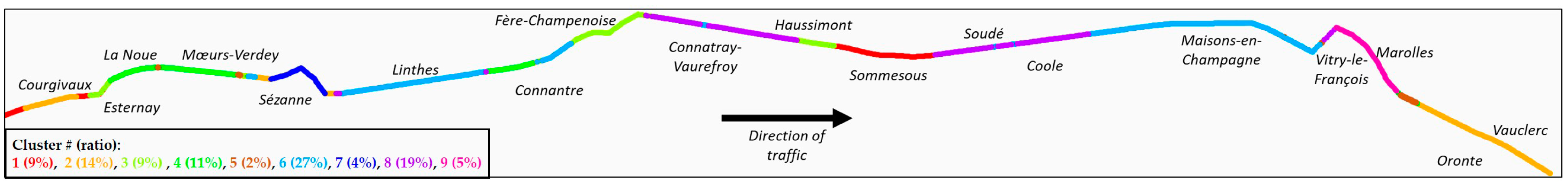Figure 10 directly presents all these nine clusters on the map (each color represents a cluster).

Projecting the clustering results on the map, we can see that it is mainly based on different characteristics of the road (type of pavement, type of lanes, and location: city, village, etc.).

The first cluster, represented in black on the map, contains 9% of the PRs of the NR4. It appears that the road markings in this cluster are laid on 2 × 2 lanes and two-lane single pavements in excellent condition. On these sections, some grading, interchanges, and planes are noticed.

Cluster 2, presented in yellow on the map, contains 12% of the marking lines. The pavement is generally paved with very thin modified bitumen, and is a 2 × 2 lane-divided pavement. In this cluster, there is the presence of unevenness, and the markings have exhibited rather stable evolution over time.

Cluster 3 groups together only the pavements in poor condition, and this is essentially a 2 × 2 lane-divided pavement surfaced with very thin modified bitumen.

Cluster 4 represents 11% of the road lines. A significant number of markings belonging to this cluster have poor pavement conditions. This includes markings on single four-lane roadways paved with very thin modified asphalt. The intersection in the plan is remarkable.

In cluster 5, The road markings have acceptable conditions and are primarily placed on single two-lane roadways. This is the only cluster that contains a portion of three-lane single pavement.

Cluster 6 focuses on 2 × 2 lane-divided roadways paved with very thin modified bitumen and in acceptable condition. There is a significant presence of gradients and interchanges.

Cluster 7 consists mostly of single two-lane pavement paved with pure thin bitumen in acceptable condition. It is the only cluster in which there are no special crossings, and its asphalt is the oldest of all and has the lowest daily traffic rate.

Cluster 8 is the only cluster where all road markings are in excellent condition. It contains, in particular, 2 × 2 lane-divided roads. Apart from the presence of gradients and planes in this cluster, a fairly high percentage of interchanges is noted.

Finally, cluster 9 has a significant percentage of grade separation. Single two-lane pavements and 2 × 2 lane-divided pavements, semi-gritty bitumen, and acceptable condition are observed. All three types of markings in this cluster show a similar pattern.

The literature shows that the Weibull distribution is suitable for analyzing the reliability of road markings. Thus, to correct the censored data, the EM algorithm is applied to each cluster j ∈ {1… g} with g = 9. For each cluster C_j, a Weibull analysis is applied using the EM algorithm presented in Section 4. The aim of this analysis is to determine the parameters of the Weibull distribution for each cluster.

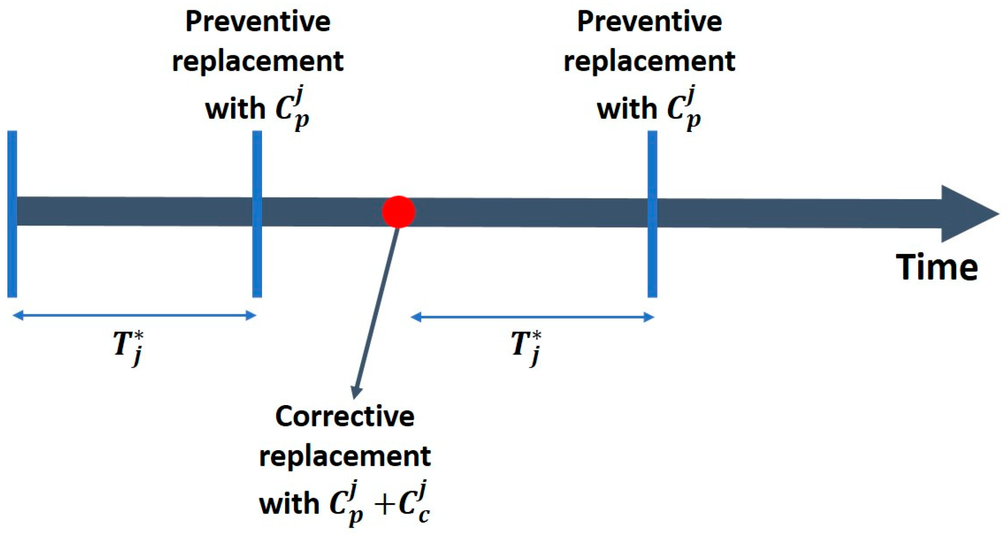
Let $C_j^p$ and $C_j^c$ be, respectively, the preventive and corrective maintenance costs of cluster C_j. The preventive maintenance cost allocated for road markings is C_p = 10 K, and the corrective maintenance cost is arbitrarily defined as C_c = 3∗C_p. This global budget is distributed equitably according to the size of the clusters. With these costs in mind, the optimal maintenance path $T_j^{*}$ is defined using age-based maintenance.

Table 1. Weibull parameters of the broken center line.

Cluster—Numbers (Frequency)	Lifetime Model	Mean Time to Failure (Months)	Optimum Replacement (Months)
1–94 (9%)	$𝒲$(21.84, 2.01)	19	11
2–140 (12%)	$𝒲$(14.89, 1.14)	14	14
3–111 (11%)	$𝒲$(19.54, 1.50)	18	13
4–111 (11%)	$𝒲$(19.46, 1.48)	18	14
5–16 (2%)	$𝒲$(11.13, 1.43)	10	8
6–270 (27%)	$𝒲$(19.72, 1.56)	18	12
7–40 (4%)	$𝒲$(18.42, 1.43)	17	14
8–188 (19%)	$𝒲$(10.85, 1.19)	10	18
9–48 (5%)	$𝒲$(14.45, 1.14)	16	14

,

Table 2. Weibull parameters of the emergency line.

Cluster—Numbers (Frequency)	Lifetime Model	Mean Time to Failure (Months)	Optimum Replacement (Months)
1–94 (9%)	$𝒲$(23.80, 2.02)	21	12
2–140 (12%)	$𝒲$(29.12, 1.95)	26	15
3–111 (11%)	$𝒲$(24.19, 1.26)	22	28
4–111 (11%)	$𝒲$(15.93, 1.80)	14	9
5–16 (2%)	$𝒲$(25.34, 1.97)	22	13
6–270 (27%)	$𝒲$(18.19, 2.01)	16	9
7–40 (4%)	$𝒲$(18.16, 1.98)	16	9
8–188 (19%)	$𝒲$(25.29, 3.24)	23	13
9–48 (5%)	$𝒲$(13.75, 1.15)	13	13

and

Table 3. Weibull parameters of the median strip line.

Cluster—Numbers (Frequency)	Lifetime Model	Mean Time to Failure (Months)	Optimum Replacement (Months)
1–94 (9%)	$𝒲$(30.34, 6.64)	28	19
2–140 (12%)	$𝒲$(32.81, 1.74)	29	18
3–111 (11%)	$𝒲$(26.60, 7.38)	25	17
4–111 (11%)	$𝒲$(24.79, 1.55)	22	16
5–16 (2%)	$𝒲$(32.23, 0.64)	45	45
6–270 (27%)	No median strip line
7–40 (4%)	$𝒲$(20.24, 4.27)	18	11
8–188 (19%)	No median strip line
9–48 (5%)	$𝒲$(20.94, 0.93)	22	22

show the Weibull parameters α_j and β_j of each cluster C_j and the optimal maintenance replacement path for each of the three lines (respectively, broken center line, emergency line, and median strip line). Note that colors in the first column refer to the clustering of the roadmap introduced in Figure 10.

The first column presents the number of the PRs that belong to each cluster with their frequency. The second one shows the associated Weibull parameters estimated by the EM algorithm. The third column presents the average operating time, and the last one lists the optimum replacement period associated with each cluster.

The replacement interval for the axial line varies between 8 and 18 months, that of the EL varies between 9 and 28 months, and that of the MSL varies between 11 and 45 months. The difference in replacement frequency is due to the nature of the road section and its location.

As an illustration, we take the first cluster as an example. It represents 9% of the PRs of NR4. The lifetime model associated with the BCL is Ω(21.84, 2.01). The preventive maintenance cost is estimated to be 940 units, and the corrective maintenance cost is defined as three times the preventive cost. According to the age-based replacement strategy, the PRs belonging to this cluster must be replaced every 19 months. The same methodology is applied to the other lines, which shows that the EL and MSL can be replaced every 12 and 19 months, respectively.

According to Tidjani et al., the clustering algorithm is followed by a FAMD to analyze the clusters or the strategic maintenance areas [33]. The FAMD proposes data management and identifies different correlations between variables. However, the FAMD considers only the CBL and EL because those of the MSL are not available everywhere on NR4.

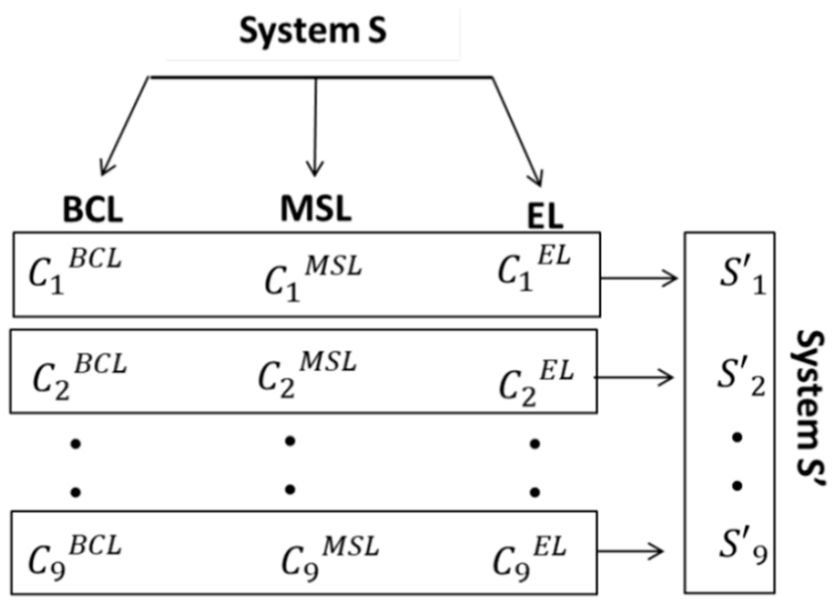
To minimize the preventive maintenance cost of the system S, we assume that each cluster represents a component of a new system denoted S′. Then, S′ is a system consisting in nine subsystems, S₁′, S₂′ … S₉′, construed as illustrated in Figure 11.

To minimize the preventive maintenance cost, the grouping methodology presented in this paper is applied to the components of each subsystem S_i′, where i ∈ {1… 9}. The aim is to determine an optimal maintenance time for replacing the three types of road markings (BCL, EL, and MSL).

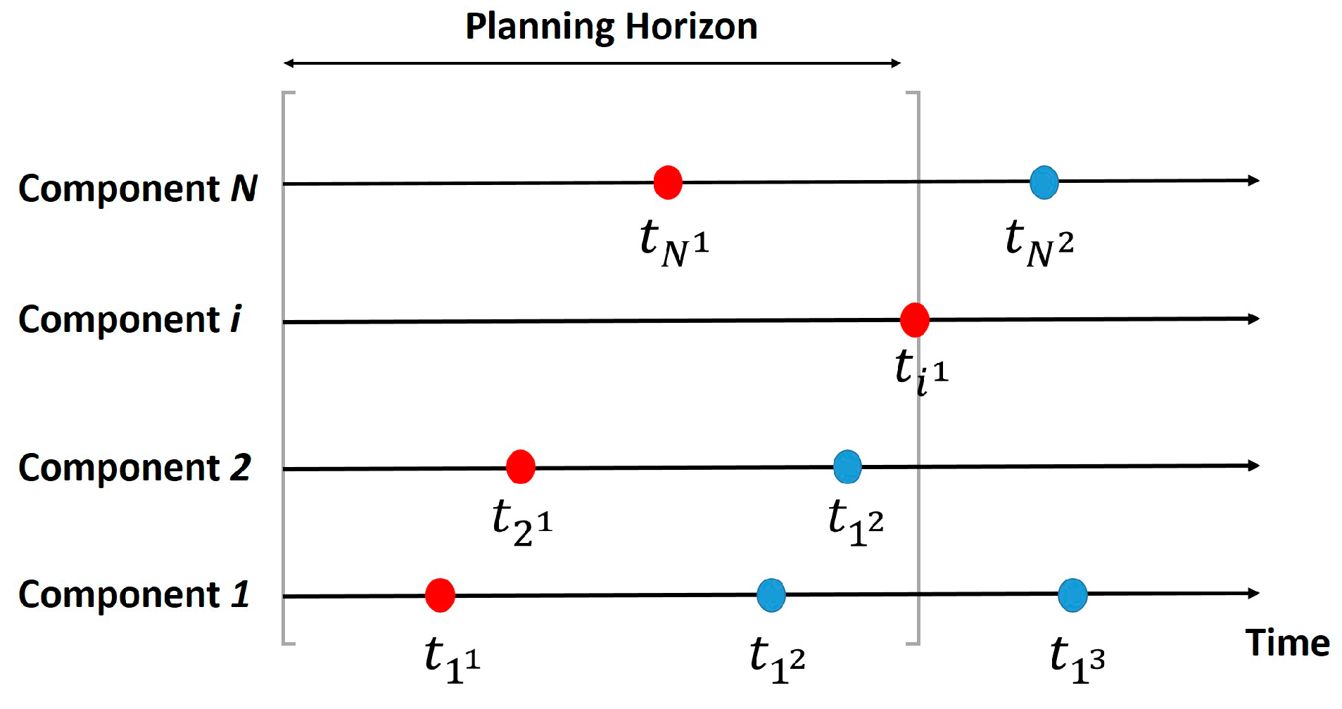
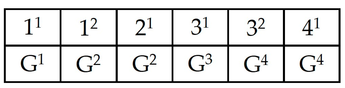
It is assumed that the components have just been held and that the planning time fence starts at time t = 0 (T_begin = 0). This strategy is applied to the rst subspace, and the planning horizon thus becomes HZ = [0,19]. At this horizon, each component must be replaced only once. For determining the optimal grouping structure, the previously introduced GA presented is considered.

Then, an initial population has to first be generated, and then the GA can be applied. The maintenance actions over the planning horizon are {1⁽¹⁾, 2⁽¹⁾, 3⁽¹⁾}. As an illustration, we consider two examples of grouping structures with two groups: G¹ = {1⁽¹⁾, 3⁽¹⁾} and G² = {2⁽¹⁾} or G¹ = {1⁽¹⁾, 2(1)} and G² = {3⁽¹⁾}, as illustrated Figure 12.

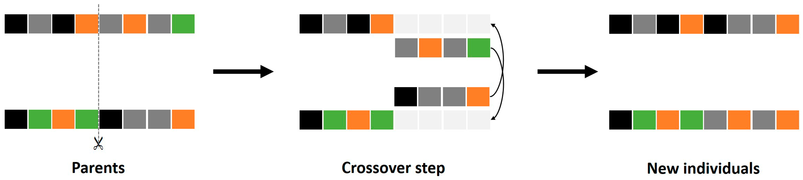
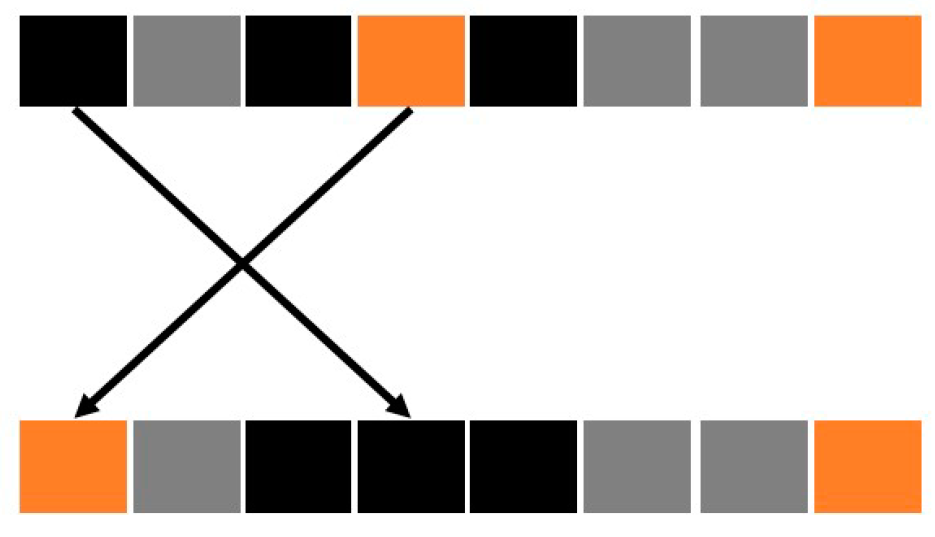
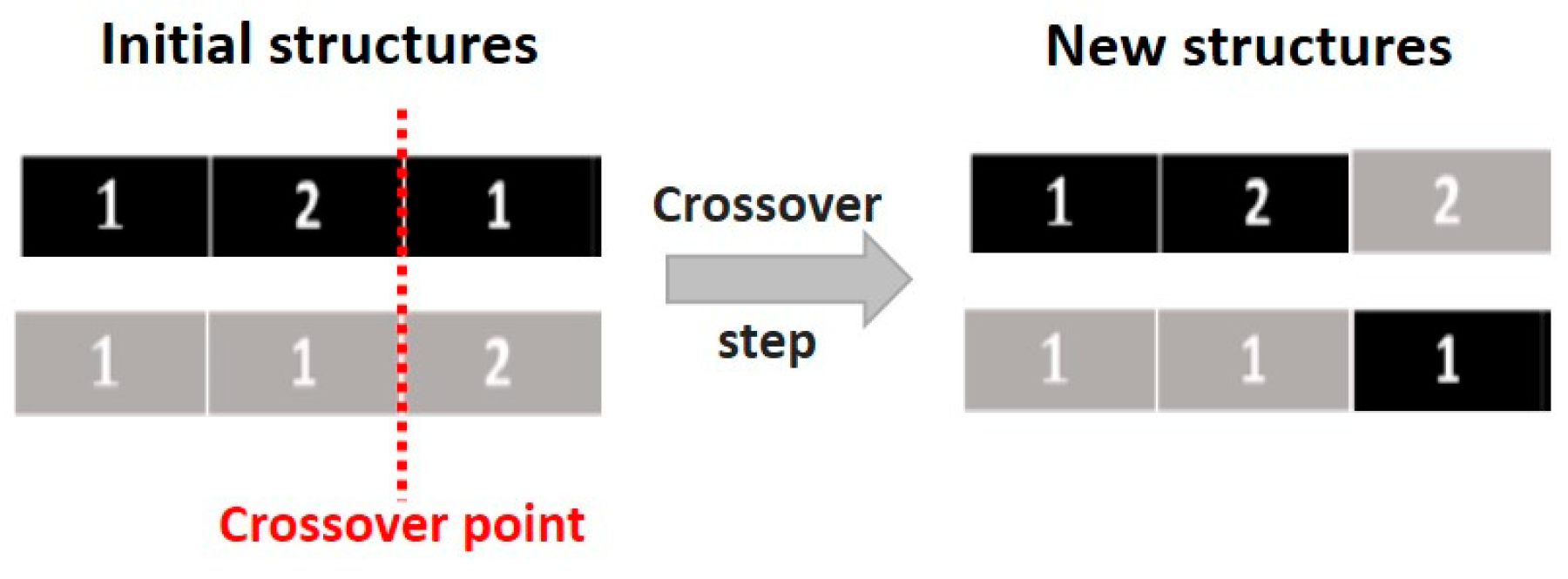
The two considered candidate solutions are encoded considering the method introduced in the previous section. Then, to generate new candidate solutions, the crossover step has to be considered. A random crossover point is chosen (e.g., point 2), and the new solutions are constructed, as represented in Figure 13.

The other steps of the GA are then applied, and other solutions are thus generated. In each iteration, the economic profit is calculated, and the best solutions are selected for the next iteration (generation). The economic benefit is calculated for each solution, and the optimal one is the candidate with the greatest total economic benefit.

Table 4. Total economic profit according to each solution candidate.

Optimal Grouping Structure	Optimal Grouping Time	TEP
{11, 21}, {31}	11, 19	247.25
{21, 31}, {11}	15, 11	113.18
{11, 31}, {21}	14, 12	62.07
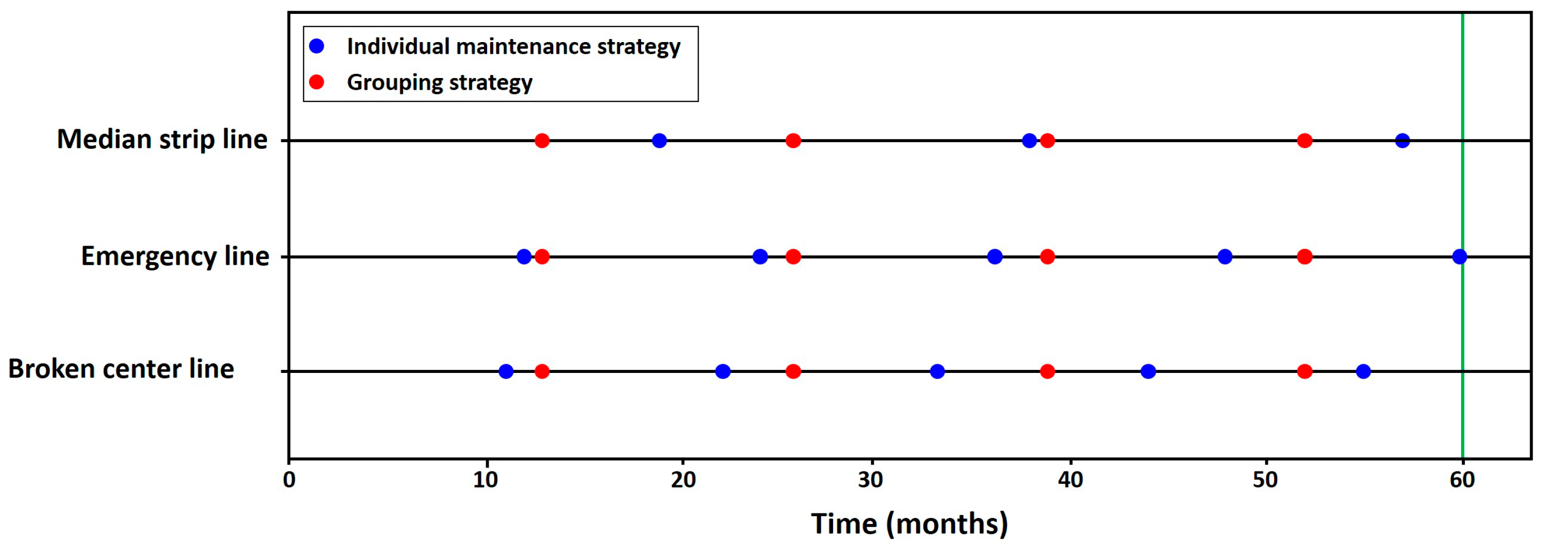
{11, 21, 31}	13	291.58

shows the optimal grouping structure for each iteration and the associated economic profit with the optimal grouping time. The best economic profit is obtained when all the maintenance actions are performed 13 months after the last replacement. This represents a 10% gain in the total maintenance cost.

To evaluate the reliability of the system in the case of grouped maintenance, we apply the maintenance strategies over a planning horizon of 60 months (5 years). Figure 14 presents a comparison between the individual maintenance plan and one with a grouping strategy. The blue points indicate the maintenance action for the individual optimal plan, and the red ones are the maintenance times for the grouped strategy. For this cluster, each component is maintained only once per cycle, and the cluster plan indicates that all three components can be maintained simultaneously every 13 months.

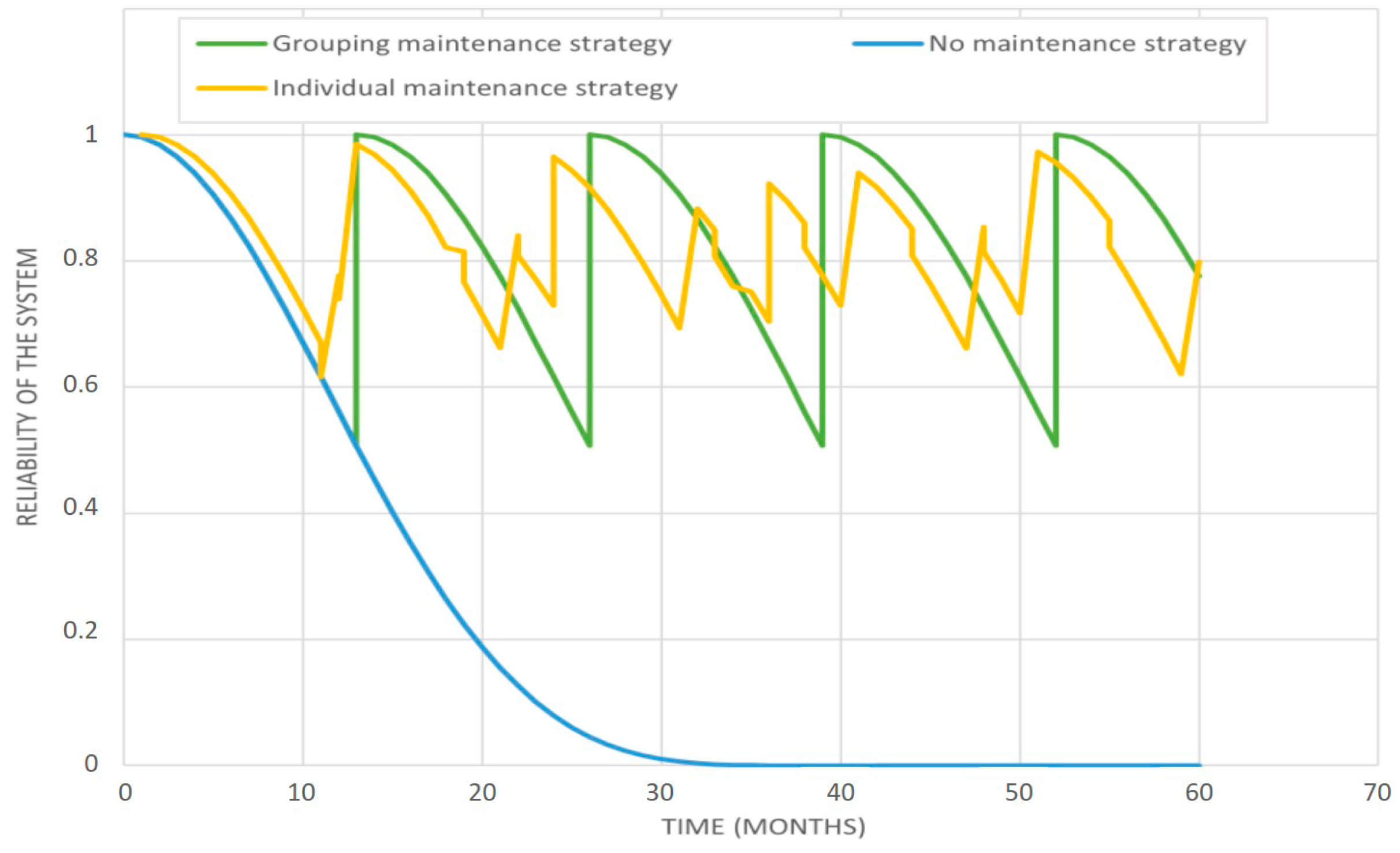
To assess the effectiveness of the bundled maintenance plan, the reliability of the system was studied under three different maintenance strategies, as shown in Figure 15:

• Without maintenance: no maintenance action is performed over the planning horizon;
• Individual maintenance: each component i is maintained at time T_i* according to the optimal individual strategy introduced in Section 5;
• Grouped maintenance: the proposed static grouped maintenance strategy is employed.

The blue graph represents the reliability of the system when no maintenance is performed. In this case, the reliability drops to 0.2 after 20 months, and the system is considered to have failed (nil reliability) after 30 months. The yellow graph represents the reliability of the system when an individual strategy is considered. The reliability varies between 1 and 0.6. After the first maintenance actions, the reliability is no longer equal to 1 because the components are no longer maintained simultaneously. Since the maintenance times are quite close (11, 12, and 19 months), reliability remains high. Finally, the green curve shows the behavior of the reliability when a grouping strategy is applied. In this case, the reliability of the system remains periodic: the three marker lines are maintained simultaneously, and their age is initialized to 0 after each replacement. 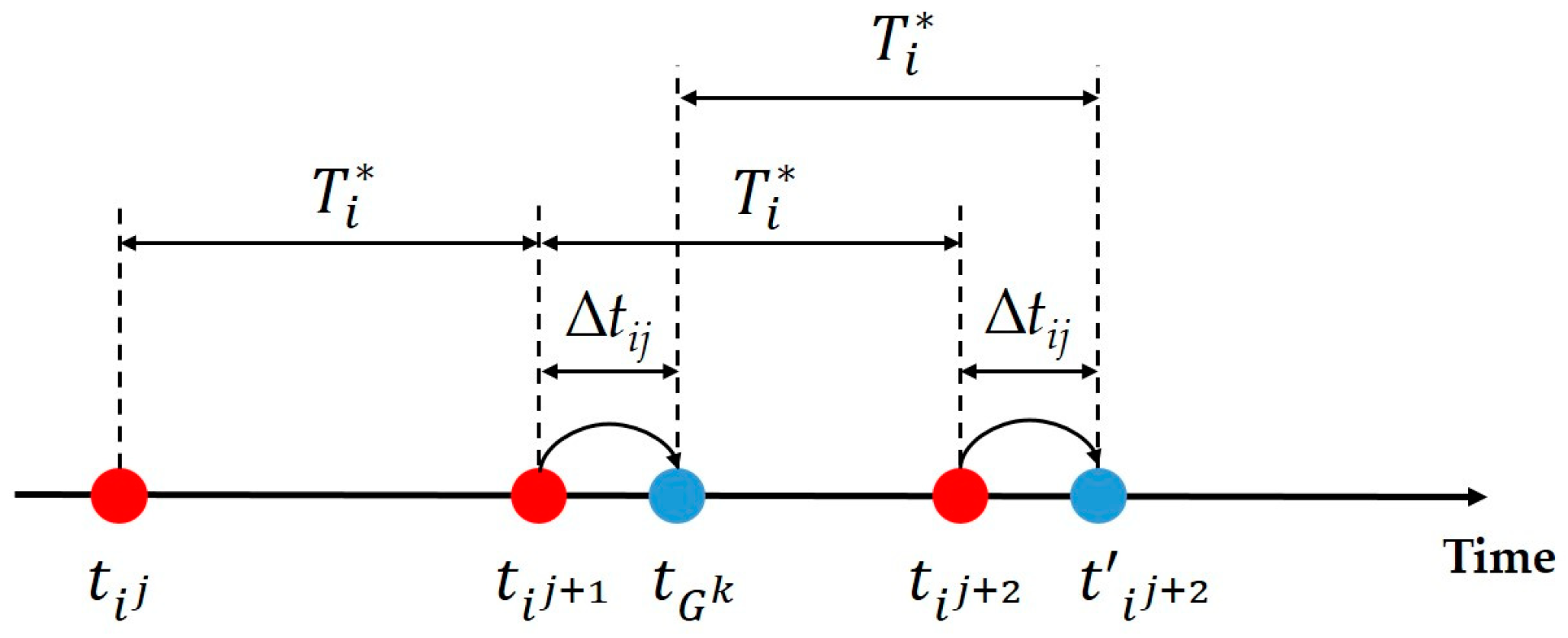As the maintenance instants are moved after each replacement (as presented in Figure 4), the same time interval between maintenance actions is always considered, hence the periodicity of reliability.

The green curve encompasses the yellow one. Even if in the case of grouped maintenance, we tolerate a lower reliability than in the case of a strategy with individual maintenance, but from an economic perspective, we save 10% of the budget allocated to maintenance for each cycle. In this case, without any constraints imposed by the infrastructure manager, the grouping strategy remains the most interesting. Moreover, both approaches have the same mean value for reliability, and even if the individual approach provides a better variance, it is easy to understand that the availability of infrastructure will be optimized with the grouped approach.

Table 5. Total economic profit according to each solution candidate for cluster 5.

Cluster	Optimal Grouping Structures	Optimal Grouping Times	TEP	TEP Gains (%)
2	{11, 21, 31}	16	482.44	+17%
3	{11}, {12}, {21, 31}	13, 26, 19	216.36	+12%
4	{11, 31}, {21}	11.9	113.89	+9%
5	{11, 21}, {12, 22},{13, 23}, {14},{15, 31}	9, 18, 27, 36, 45	542.1	+16%
6	{11, 21}	9	52.47	+7%
7	{11, 21, 31}	10	215.48	+10%
8	{11, 21}	14	47.1	+7%
9	{11, 21, 31}	12	239.13	+10%

shows the optimal grouping strategy for each cluster and the associated economic profit. We consider cluster 5 as an example. On the planning horizon, the EL and the BCL have to be replaced many times. Whenever maintenance actions are grouped together, the next maintenance instances are shifted, and only those remaining on the planning horizon are taken into consideration. For this cluster, the grouping strategy allows a 16% gain in the TEP in comparison with an individual optimization approach.

In

Table 6. Average reliability for each cluster with respect to the considered maintenance strategy.

Cluster	No Maintenance	Individual Optimization	Grouped Strategy
1	0.24	0.83	0.83
2	0.17	0.56	0.59
3	0.2	0.54	0.66
4	0.16	0.6	0.6
5	0.11	0.39	0.42
6	0.2	0.77	0.84
7	0.17	0.71	0.79
8	0.16	0.52	0.58
9	0.1	0.31	0.51

, the average reliability for each cluster under the three considered different maintenance strategies is introduced. If no maintenance action is performed, the average reliability does not exceed 0.24%, which is perfectly understandable since the road markings performance decrease to zero and then stay null up to the end of the time horizon. We can notice that, as previously introduced, the average reliability for the considered two maintenance strategies is quite close and generally better for the grouped approach (even if we also noticed that the variance is generally better for the individual approach). However, in terms of economic perspectives, the grouped maintenance strategy systematically provides an interesting economic benefit. In this case, the grouped maintenance strategy is more interesting. Moreover, we noticed that the availability of infrastructures is necessarily better with grouped actions than with individual strategies, which is a not-negligible advantage.

9. Conclusions and Prospects

The aim of this study was to determine the optimal maintenance plan for all the road markings of an infrastructure. For this, we first proposed a feedback data process to identify several degradation profiles and cluster the infrastructure. The systems considered in this study are periodically inspected. The monitoring data are generally triply censored with right, left, and interval censoring. In this paper, the proposed maintenance grouping policy was applied to road markings by considering road infrastructure as a three-component serial system. In our case study, the whole infrastructure was considered as a set a sections characterized by their own degradation process (influenced by the typology of the section, the nature of the pavement, its location, etc.). To group the road sections that degrade in the same way, the unsupervised clustering algorithm AHC was applied. This clustering grouped the road marking lines into nine clusters. Each cluster grouped the components that have the same evolution or degradation over time. In this case, instead of correcting the censoring and assigning a maintenance plan for each marking, the proposed analysis was applied to each cluster. We thus applied an extension of the EM algorithm to estimate the failure time and assign a Weibull distribution to each cluster.

Then, the grouped maintenance strategy started by identifying an optimal individual maintenance period for each cluster. An age-based maintenance replacement was considered in this paper. Since simultaneously performing all maintenance tasks is not always the optimal solution, a GA was used to determine the optimal solution by grouping several actions. This algorithm offers better results than dynamic programming and entails a reasonable execution time. This grouping strategy considers budget constraints and the previously described life duration model. It demonstrated a significant decrease in the budget allocated to preventive maintenance. The advantages and strengths of the proposed process lie in the fact that it can address highly censored data. This type of data is often encountered when a system is periodically inspected and maintained. The maintenance process proposed in this paper is based on individual optimization with clustering of the monitoring database. In our case study, the clustering was very useful to the infrastructure manager because it helped to better understand the road network behavior.

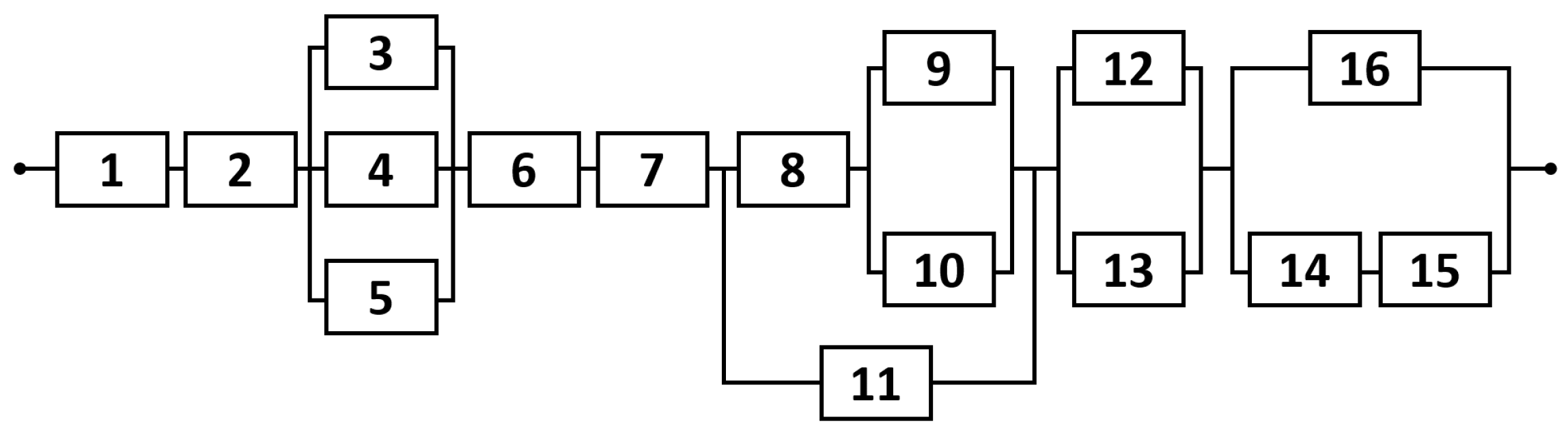
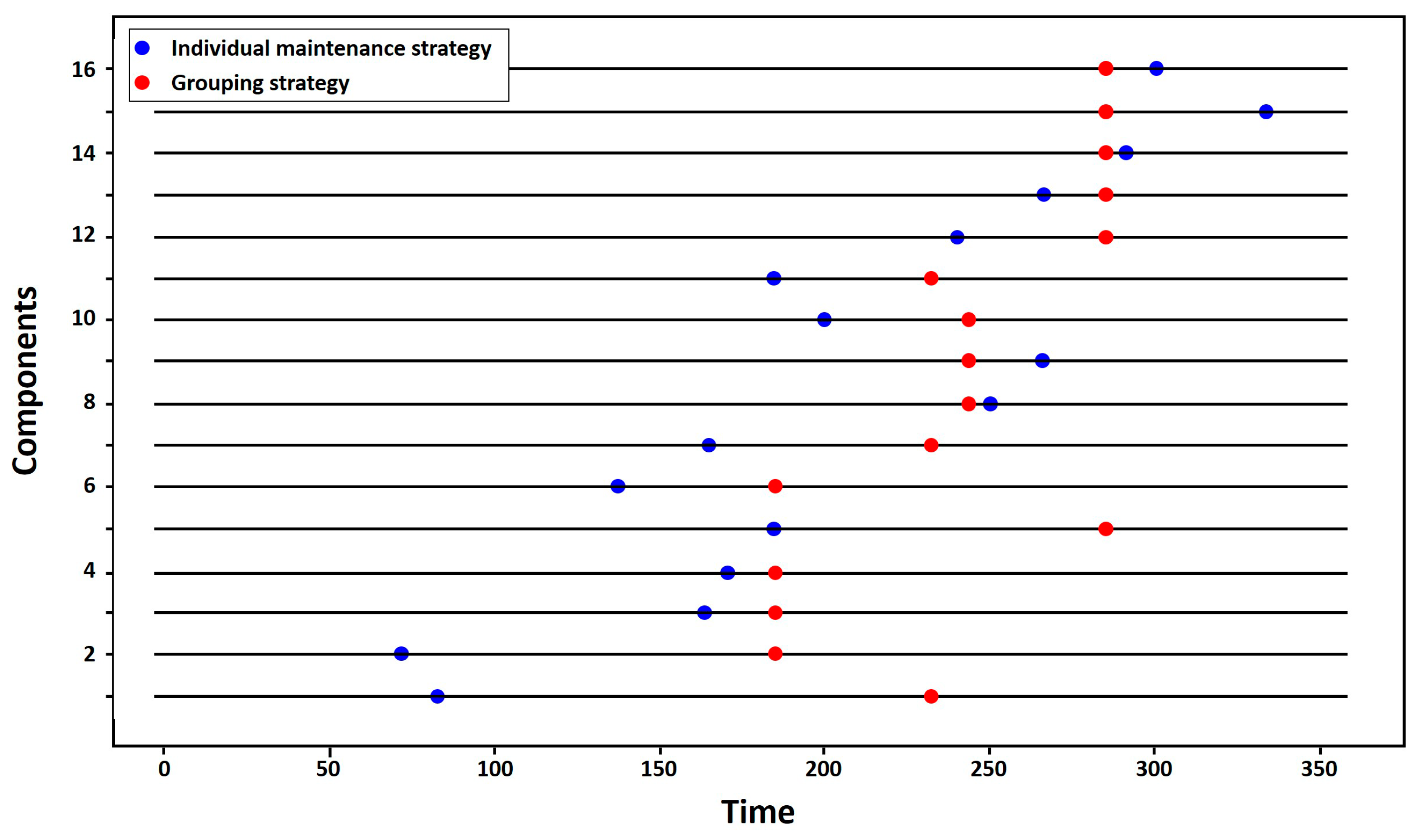
Although the case study, which is the main objective of this work, is a simple system, our approach has demonstrated its applicability to even more complex structures through its application to a 16-component complex structure system from the literature.

On the other hand, the strategy has some limitations. First, the optimal grouped maintenance clearly depends on the planning horizon, which, in our case, is finite. The definition of this horizon, in an optimal way, could depend on budget and availability constraints. Future works could deal with defining the value of the time horizon with respect to such constraints. Moreover, the literature has shown that, in general, the GA is the most-used algorithm to optimize a grouping maintenance strategy; however, other works such as [29] have shown that other optimization approaches offer interesting solutions (mainly in terms of complexity). Indeed, GA generally faces some limitations when the system has a complex structure, and other algorithms such as PSO and clustering optimization seem to be more efficient and could be added to our work.

Finally, the last limitation, but not the least important, deals with taking constraints into account in the optimization process. The next step of this study is currently in progress through two new PhD projects, taking into account new constraints such as maintenance action durations and resource constraints (maintenance staff and maintenance equipment), but also some availability constraints connected with operating needs. Indeed, the literature review underlines that no previous study has considered more than one of these constraints in its maintenance optimization process for complex systems.

References

1. Pinciroli, L.; Baraldi, P.; Zio, E. Maintenance optimization in industry 4.0. Reliab. Eng. Syst. Saf. 2023, 234, 109204. [Google Scholar] [CrossRef]
2. Dekker, R.; Wildeman, R.E.; Van Egmond, F.A. A review of multi-component maintenance models with economic dependence. Math. Methods Oper. Res. 1997, 45, 411–435. [Google Scholar] [CrossRef] [Green Version]
3. Faddoul, R.; Raphael, W.; Chateauneuf, A. Maintenance optimization of series systems subject to reliability constraints. Reliab. Eng. Syst. Saf. 2018, 180, 179–188. [Google Scholar] [CrossRef]
4. Wildeman, R.E.; Rommert, D.; Smit, A.C.J.M. A dynamic policy for grouping maintenance activities. Eur. J. Oper. Res. 1997, 99, 530–551. [Google Scholar] [CrossRef] [Green Version]
5. Vu, H.C.; Do, P.; Barros, A.; Berenguer, C. Maintenance grouping strategy for multi-component systems with dynamic contexts. Reliab. Eng. Syst. Saf. 2014, 132, 233–249. [Google Scholar] [CrossRef]
6. Redondin, M.; Bouillaut, L.; Daucher, D. A clustering-based approach to segment a pavement markings line. Int. J. Perform. Eng. 2020, 16, 1497–1508. [Google Scholar]
7. Luce, S. Choice criteria in conditional preventive maintenance. Mech. Syst. Signal Process. 1999, 13, 163–168. [Google Scholar] [CrossRef]
8. Mobley, R.K. An Introduction to Predictive Maintenance, 2nd ed.; Elsevier: Paris, France, 2002. [Google Scholar]
9. Hunter, M.L. Climate change and moving species: Furthering the debate on assisted colonization. Conserv. Biol. 2007, 21, 1356–1358. [Google Scholar] [CrossRef]
10. Redondin, M.; Daucher, D.; Bouillaut, L. An EM approach for a Weibull analysis of pavement markings in context of a strong censored life time. Int. J. Perform. Eng. 2021, 17, 333–342. [Google Scholar] [CrossRef]
11. Celeux, G.; Chauveau, D.; Diebolt, J. On Stochastic Versions of the EM Algorithm. Ph.D. Thesis, INRIA Research Program, Versailles, France, 1995. [Google Scholar]
12. Marschner, I.C. Miscellanea On stochastic versions of the algorithm. Biometrika 2001, 88, 281–286. [Google Scholar] [CrossRef]
13. Gelman, A.; Carlin, J.B.; Stern, S.H.; Rubin, D.B. Bayesian Data Analysis, 3rd ed.; Taylor & Francis: New York, NY, USA, 2013. [Google Scholar]
14. Congdon, P. Bayesian Statistical Modelling, 2nd ed.; John Wiley and Sons: New York, NY, USA, 2007. [Google Scholar]
15. Ducros, F.; Pamphile, P.; Université Paris Sud, Orsay, France. Maintenance Cost Forecasting for a Fleet of Vehicles. Personal communication, 2019. [Google Scholar]
16. Nakagawa, T. A summary of imperfect preventive maintenance policies with minimal repair. RAIRO-Oper. Res. 1980, 14, 249–255. [Google Scholar] [CrossRef] [Green Version]
17. Valdez-Flores, C.; Feldman, R.M. A survey of preventive maintenance models for stochastically deteriorating single-unit systems. Nav. Res. Logist. 1989, 36, 419–446. [Google Scholar] [CrossRef]
18. Wang, H. A survey of maintenance policies of deteriorating systems. Eur. J. Oper. Res. 2002, 139, 469–489. [Google Scholar] [CrossRef]
19. Barlow, R.E.; Proshan, F. Mathematical Theory of Reliability, 1st ed.; John Wiley: New York, NY, USA, 1965. [Google Scholar]
20. Zhang, Y.L.; Yam, R.C.; Zuo, M.J. Optimal replacement policy for a deteriorating production system with preventive maintenance. Int. J. Syst. Sci. 2001, 32, 1193–1198. [Google Scholar] [CrossRef]
21. Pham, H.; Wang, H. Imperfect maintenance. Eur. J. Oper. Res. 1996, 94, 425–438. [Google Scholar] [CrossRef]
22. Saada, Y.; Yahyaoui, E.M.; Ouadoudi, N.; Skouri, R.; Daya, A. Mathematical Simulation Methods to Evaluate the Effects of Actions on Conditional Preventive Maintenance of Complex Systems. Int. J. Eng. Res. Afr. 2018, 35, 38–59. [Google Scholar] [CrossRef]
23. Guan, J.; Yang, X.; You, L.; Ding, L.; Cheng, X. Multi-objective optimization for sustainable road network maintenance under traffic equilibrium: Incorporating costs and environmental impacts. J. Clean. Prod. 2022, 334, 130103. [Google Scholar] [CrossRef]
24. Shi, Y.; Xiang, Y.; Xiao, H.; Xing, L. Joint optimization of budget allocation and maintenance planning of multi-facility transportation infrastructure systems. Eur. J. Oper. Res. 2021, 16, 382–393. [Google Scholar] [CrossRef]
25. Zhang, X.; Gao, H. Road maintenance optimization through a discrete-time semi-Markov decision process. Reliab. Eng. Syst. Saf. 2012, 103, 110–119. [Google Scholar] [CrossRef]
26. Nguyen, H.S.H. Development of a Dynamic Grouping Maintenance Strategy for a Geographically Dispersed Production System. Ph.D. Thesis, Université de Lorraine, Nancy, France, 2019. [Google Scholar]
27. Vu, H.C.; Do, P.; Barros, A. A stationary grouping maintenance strategy using mean residual life and the Birnbaum importance measure for complex structures. IEEE Trans. Reliab. 2015, 65, 217–234. [Google Scholar] [CrossRef]
28. Chalabi, N.; Dahane, M.; Beldjilali, B.; Neki, A. Optimisation of preventive maintenance grouping strategy for multi-component series systems: Particle swarm based approach. Comput. Ind. Eng. 2016, 102, 440–445. [Google Scholar] [CrossRef]
29. Hanini, M.; Khebbache, S.; Bouillaut, L.; Hadji, M. Dynamic and adaptive grouping maintenance strategies: New scalable optimization algorithms. Proc. IMechE Part O J. Risk Reliab. 2022, 236, 647–660. [Google Scholar] [CrossRef]
30. Do, P.; Vu, H.C.; Barros, A.; Bérenguer, C. Maintenance grouping for multi-component systems with availability constraints and limited maintenance teams. Reliab. Eng. Syst. Saf. 2015, 142, 56–67. [Google Scholar] [CrossRef] [Green Version]
31. Jha, M.K.; Udenta, F.; Chacha, S.; Abdullah, J. Formulation and solution algorithms for highway infrastructure maintenance optimisation with work-shift and overtime limit constraints. Procedia—Soc. Behav. Sci. 2010, 2, 6323–6331. [Google Scholar] [CrossRef] [Green Version]
32. Sathyanarayanan, S.; Shankar, V.; Donnell, E.T. Pavement Marking Retroreflectivity Inspection Data: A Weibull Analysis. Transp. Res. Rec. J. Transp. Res. Board 2008, 2055, 63–70. [Google Scholar] [CrossRef]
33. Tidjani, A.; Redondin, M.; Bouillaut, L.; Daucher, D. Impact of Road Infrastructure Characteristics on Road Markings. In Proceedings of the 29th ESRA European Safety & Reliability International Conference ESREL’19, Hannover, Germany, 22–26 September 2019. [Google Scholar]
34. Derbe, A.; Boujelbene, Y. Automatic Classification and Analysis of Multiple-Criteria Decision Making. In Proceedings of the 8th International Conference on Sciences of Electronics, Technologies of Information and Telecommunications SETIT’18, Maghreb, Tunisia, 18–20 December 2018. [Google Scholar]
35. Duchesnay, E. Statistics and Machine Learning in Python, 1st ed.; Springer: Berlin/Heidelberg, Germany, 2019. [Google Scholar]
36. Pradhan, B.; Kundu, D. Analysis of interval-censored data with Weibull lifetime distribution. Indian J. Stat. 2014, 76, 120–139. [Google Scholar] [CrossRef]
37. Shapiro, J. Genetic algorithms in machine learning. In Proceedings of the Advanced Course on Artificial Intelligence, Chania, Greece, 5–16 July 1999; pp. 146–168. [Google Scholar]
Figure 1. General view of the proposed process for a grouping maintenance strategy of a multicomponent system, periodically observed.
Futuretransp 03 00044 g001
Figure 2. Example of the age-based replacement strategy.
Futuretransp 03 00044 g002
Figure 3. Example of planning horizon for an N component system.
Futuretransp 03 00044 g003
Figure 4. Example of changing execution time process.
Futuretransp 03 00044 g004
Figure 5. Example of a grouping structure array for a 4-component system, considering 6 maintenance actions.
Futuretransp 03 00044 g005
Figure 6. Crossover step.
Futuretransp 03 00044 g006
Figure 7. Mutation step.
Futuretransp 03 00044 g007
Figure 8. System with 16 components used by Vu et al. [5].
Futuretransp 03 00044 g008
Figure 9. Grouping strategy for the 16 components system.
Futuretransp 03 00044 g009
Figure 10. Results of an AHC on reflectivity data of RN4.
Futuretransp 03 00044 g010
Figure 11. Modeling of the road markings system.
Futuretransp 03 00044 g011
Figure 12. Examples of grouping structures with two groups.
Futuretransp 03 00044 g012
Figure 13. Illustration of the crossover step.
Futuretransp 03 00044 g013
Figure 14. Individual and grouped maintenance strategies for cluster 1.
Futuretransp 03 00044 g014
Figure 15. Reliability of the system, in respect of time (in months), under three maintenance strategies for cluster 1.
Futuretransp 03 00044 g015