Real-Time Suitable Predictive Control Using SPaT Information from Automated Traffic Lights

Abstract

Traffic intersections throughout the United States combine fixed, semi-actuated, and fully actuated intersections. In the case of the semi-actuated and actuated intersections, uncertainties are considered in phase duration. These uncertainties are due to car waiting queues and pedestrian crossing. Intelligent transportation systems deployed in traffic infrastructure can communicate Signal and Phase Timing messages (SPaT) to vehicles approaching intersections. In the connected and automated vehicle ecosystem, the fuel savings potential has been explored. Prior studies have predominantly focused on fixed time control for the driver. However, in the case of actuated signals, there is a different and significant challenge due to the randomness caused by uncertainties. We have developed a predictive control using the SPaT information communicated from the actuated traffic intersections. The developed MPC-based algorithm was validated using model-based design platforms such as AMBER^®, Autonomie^®, MATLAB^®, and SIMULINK^®. It was observed that the proposed algorithm can save energy in a single phase, in multiple phase scenarios, and in compelled stopping at stop signs when employed considering communications.

1. Introduction and Literature Review

United States Energy Consumption Administration has shared that the Transportation sector consumes more than 150 quadrillions of Btu energy [1]. Presently, the majority of vehicles are still gasoline-powered vehicles. Fossil-fuel-based vehicles cause sustainability concerns and have detrimental environmental effects due to emissions. To reduce transportation energy consumption, the market for Electric Vehicles (EVs) and Hybrid Electric Vehicles (HEVs) is rapidly growing. In addition, advanced technologies in transportation control, Vehicle-to-Vehicle (V2V), and Vehicle-to-Infrastructure (V2I) communications are being explored to reduce the energy consumption of Connected and Automated Vehicles (CAV). The CAV environment can be revolutionary for the automotive industry. Typically, CAVs have better convenience, safety, and the capabilities of vehicle-to-infrastructure and vehicle-to-vehicle communications, which provide opportunities to suggest driving speeds. The authors in [2] provide an analysis of accidents that could have been avoided with the help of CAV in the real world. Discussions on the benefits of communication that can be utilized to maneuver more safely are put forward. Advanced Driver Assist System (ADAS) development utilizing CAV-based information sharing to avoid accidents and save lives is analyzed in [3]. Using CAV data, turning movement estimation using Kalman filters is explored in [4]. The authors claim it is cost-efficient and effictive to create signal and phase timing plans.

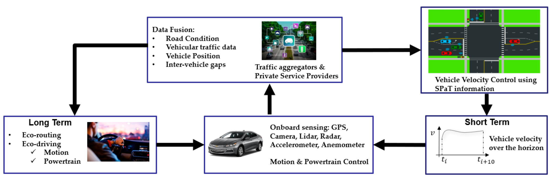
A big-data-based short-term traffic forecasting technique is shared in [5]. Velocity control using these promising technologies provides an opportunity for energy savings. Figure 1 depicts a hierarchical system consisting of long-term and short-term control strategies. In the CAV environment, as shown in Figure 1, the control system can contain multiple layers that utilize historical and real-time information. Long-term control strategies aim to provide solutions for eco-routing and eco-driving for a trip. Short-term control strategies consider the immediate future’s planning and control for the system considering uncertainties. A two-level hierarchal cooperative control technique that fixed phase duration traffic signal and HEV energy management was used to reduce energy consumption [6]. An overview of various intelligent controls of vehicles to achieve energy savings is shared in [7]. Data about road conditions, overall vehicular traffic, inter-vehicle positioning, or crowding can be fused for considering long-term plans. At the same time, onboard sensors such as GPS, cameras, Lidar, Radar, and accelerometers can be employed to generate short-term strategies.

Across the traffic networks in the United States, the traffic devices which control the movements of vehicles consist of fixed duration traffic lights, semi-actuated traffic lights, and fully actuated traffic lights. Semi-actuated and fully actuated traffic lights incorporate uncertainties through sensors such as cameras and push buttons for pedestrians, available at the intersections. In addition, car waiting queues and pedestrians waiting to cross the intersection sensed by intersection sensors are used to determine the duration of red or green phases for the multiple movements defined in the intersection.

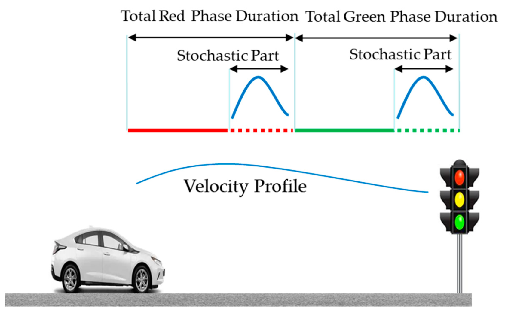
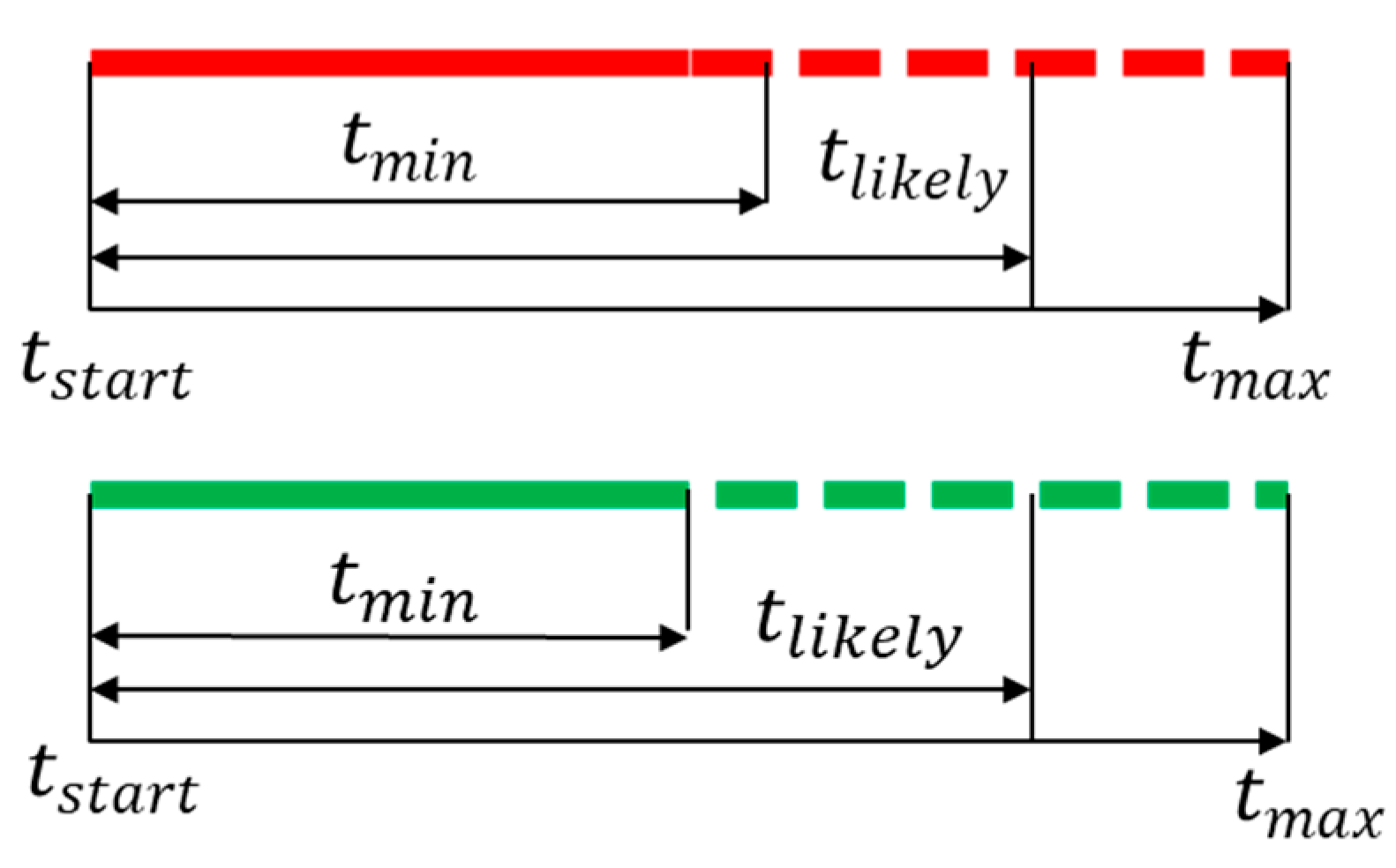
Signal phase and timing messages, popularly known as SPaT messages, can consist of information such as the current phase $\left(P_c\right)$, start time $\left(t_{start}\right)$, minimum end time $\left(t_{min}\right)$, likely end time $\left(t_{likely}\right)$, and maximum end time $\left(t_{max}\right)$ [8]. Pictorial time-based descriptions for red phase duration and green phase are shown in Figure 2 and Figure 3. Figure 2 shows that the vehicle velocity control has to perform maneuvers considering the stochastic nature of the phase duration for the green and red phase. Figure 3 shares the nature of the three ends of phase time estimations or the remaining time in the phase estimations. The estimations are available from the beginning of the phase. However, the estimation can keep changing and end up at different values than the estimations predicted at the beginning of the phase. With the developments in traffic infrastructure, cellular communications, and dedicated short-range communication (DSRC), signal phase and timing messages can be communicated to vehicles approaching the intersections. In CAV ecosystems, the availability of signal phase information supports the investigation of the fuel and/or energy savings potential. Prior studies have mainly focused on fixed time traffic signal controls for the driver. However, in the case of actuated signals or semi actuated signals, there are significant challenges due to the randomness caused by uncertainties.

Asadi and Vahidi [9] identified feasible green phases to find the target velocity considering pre-timed fixed traffic phase intervals. The article studied pre-timed fixed traffic intersections. The impact on traffic due to vehicle crawling speed to pass through the green phase was ignored. Mahler and Vahidi [10] developed an algorithm based on dynamic programming in the spatial domain to carry out green waving using probabilistic prediction for actuated traffic signal timings. In the work published by Ibrahim et al. [11], estimating phase duration for SPaT messages by collecting data for 2 weeks to a month and more was achieved by minimizing a loss function. This development supports the assumption that there can be an average duration for the red and green phases. In article [12], the authors developed a statistical methodology to populate the SPaT messages as per SAE J2735. A four-mile corridor was studied to incorporate the uncertainties due to pedestrian actuation and different timing plans. The study signifies the need and importance of confidence interval accuracy and consistency from the beginning to the end of the phase.

Instantaneous SPaT messages can be used along with historical information for prediction. For actuated signals, Hao et al. [13] demonstrated the approach and departure technique, which uses cosine/sine speed equations and a pre-defined deceleration speed profile. For decision making the algorithm implements a conservative strategy by using the minimum end time of the green signal. While the maximum end time of the red signal is used. The algorithm does not optimize the trajectory, but creates an acceleration profile based on cosine speed. Using dynamic programming and data-driven chance constraints, Sun et al. [14] developed a long term eco-driving algorithm. The solution does not consider safety concerns due to probabilistic constraint satisfaction. Vehicles may be allowed to pass the traffic intersection during the red phase, causing safety concerns. Rostami-Shahrbabaki, Majid et al. [15] have developed a speed advisory system for the mixed-traffic condition. A reinforcement learning approach was developed and employed to simulate real-world traffic. The results shared flow efficiency benefits and emissions reduction opportunities. In article [16], the authors developed an eco-driving profile for an electric vehicle, but the traffic conditions around the vehicle while driving on roads were not considered. A decentralized hierarchical HEV energy management strategy was described in [17]. Velocity profile generation for the real-time predictive control of a hybrid powertrain was discussed in [18]. An MPC-based energy management framework assuming a cloud-based traffic information distribution can be found in article [19]. Article [20] shares the framework and experimental results of leveraging smart connectivity and intelligence to achieve energy savings. Distance-based velocity profile optimization considers velocity and powertrain details to generate velocity predictions for the energy management of PHEV [21,22]. An MPC energy management technique utilizing lumped parameter analysis of vehicle sub-systems to save energy is given in article [23]. In article [24], an eco-approach is proposed to achieve efficiency, as well as overtaking slow-moving vehicles for trucks in fixed timing control signalized intersections. A micro-simulation-based optimization technique is discussed in [25]. Different saturation rates and green phase ratios are simulated using MATLAB and SUMO. Each vehicle is treated like a particle in a traffic flow. The traffic flow studies benefit when a larger green ratio and CAV penetration can be provided.

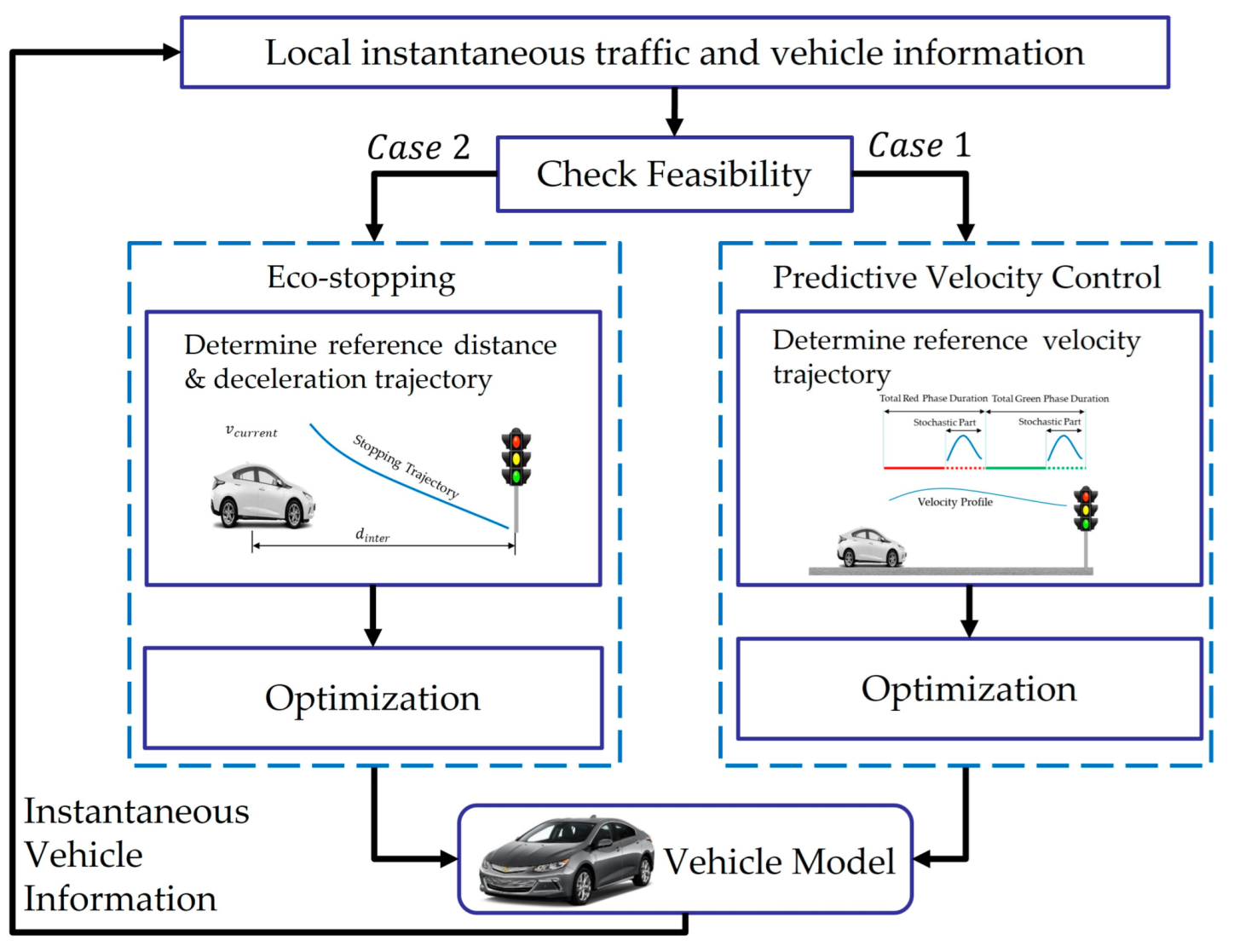
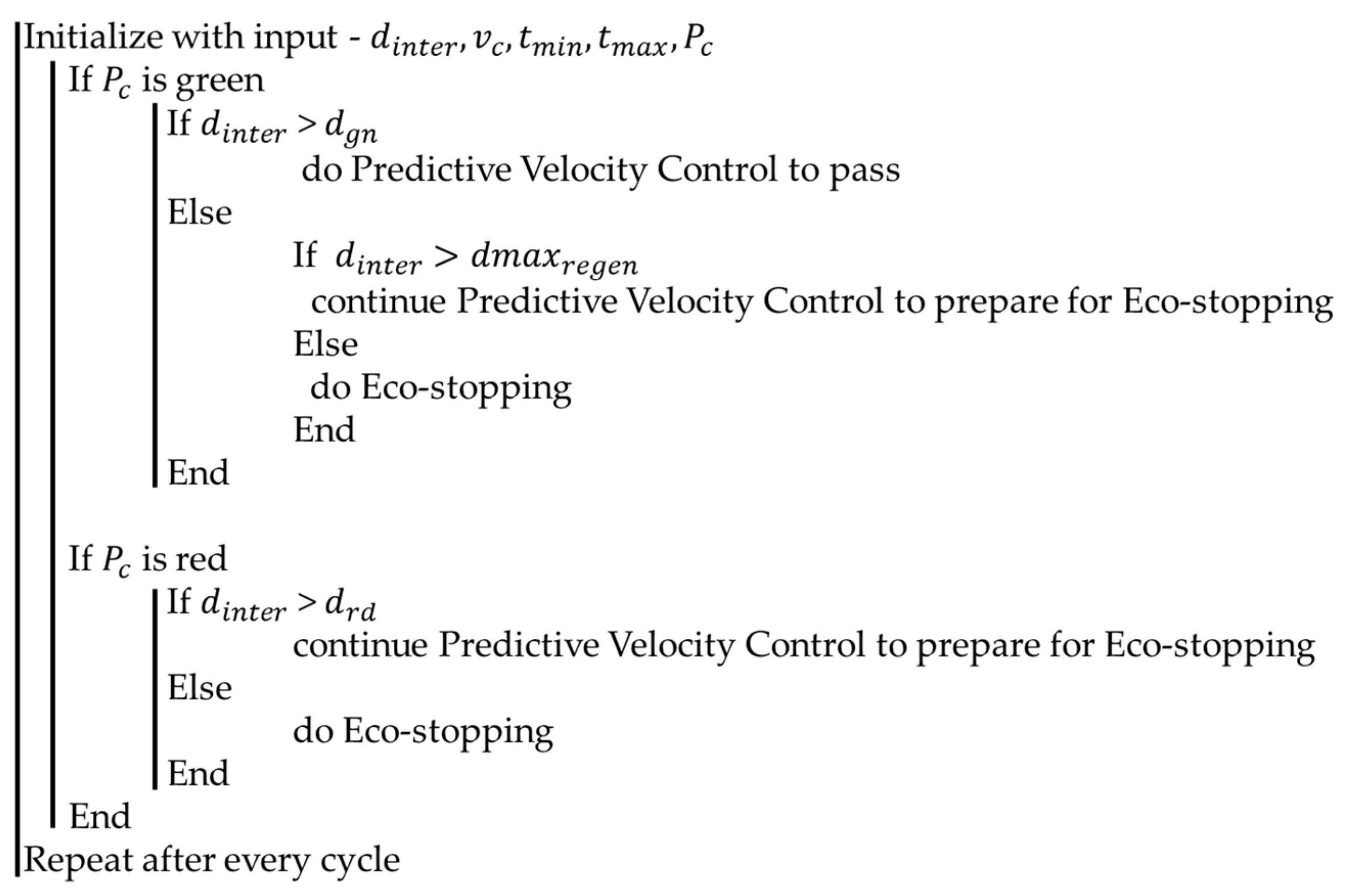
In this paper, we focus on a predictive control algorithm for vehicle velocity control and economical stopping when cruising through a traffic intersection is not feasible or safe. The major contribution of the paper is vehicle velocity control for semi-actuated and fully actuated traffic intersections, which provides non-deterministic estimations for the phase timings. Additionally, the algorithm explores the opportunity to maximize the regenerative braking energy when stopping at an intersection or a stop sign, henceforth called eco-stopping. The developed control strategies are real-time suitable. To the best of our knowledge, the framework can be utilized for electric vehicles. This aids the infrastructure development research pertaining to the electric power grid to facilitate the penetration of renewables in the power grid [26] and reduce carbon emissions due to the frugal consumption of available energy.

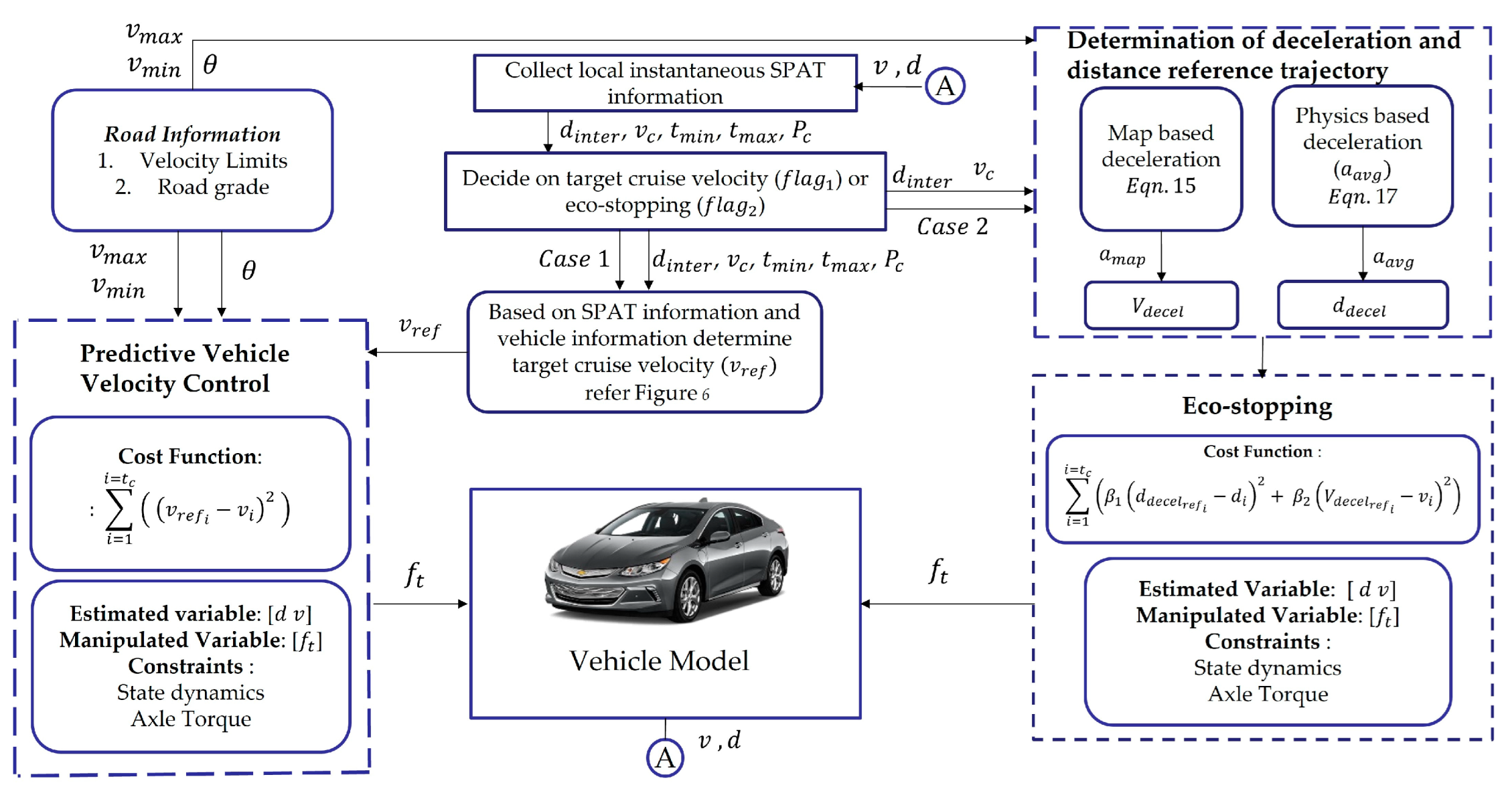
The rest of the paper is organized as follows. Section 2 describes the overall architecture and algorithms of predictive vehicle velocity control and eco-stopping. The section also includes criteria for finding the feasibility of either passing through a traffic intersection without stopping or eco-stopping to regenerate energy by exploiting the capabilities of the vehicle. Section 3 details the validation, results and discusses the results of the presented algorithms. Section 4 provides the conclusion based on the results and demonstrates how Intelligent Transport Systems can use the presented algorithms to achieve energy savings and ensure safety.

2. Predictive Control of Connected Vehicles at Automated Signalized Intersections

For safety and energy efficiency, the control system first checks the feasibility of passing a vehicle through a traffic intersection. Figure 4 provides an overview of the predictive velocity control at signalized intersections. As shown in the Figure 4, the output of the feasibility switches the applicable algorithm to optimize the vehicle velocity control decision. The control system uses the SPaT information, current vehicle velocity, and the current distance between the ego vehicle and traffic intersection to determine if the predictive control of vehicle velocity to pass through the intersection in the green phase should be performed or apply the eco-stopping algorithm to stop the vehicle efficiently. The yellow phase is considered as part of the red phase in this research for safety reasons. Case 1 represents the predictive vehicle velocity control when it is feasible to pass through the traffic intersection without stopping. Case 2 is for economical stopping with an aim to maximize energy regeneration considering vehicle limitations. To determine the applicable case, the current distance between the vehicle and traffic intersection is compared with the distance required to reach the desired velocity and location with respect to acceleration and deceleration.

2.1. Feasibility Check at Traffic Intersections

As per the available information shared through SPaT messages, a vehicle controller has to decide to either perform predictive vehicle velocity control to pass through the traffic intersection, or execute eco-stopping at every time instance $\left(t\right)$. When the current phase is green, the distance required to achieve the velocity as per the ratio of distance from the vehicle until the traffic intersection to the minimum end of phase time estimate is defined in Equation (1)

$$d_{gn}(t)=\frac{{\left(\frac{d_{inter}\left(t\right)}{t_{min}\left(t\right)}\right)}^2-v_c{\left(t\right)}^2}{2a_m}$$

(1)

where $d_{inter}$ is the distance from the vehicle to the traffic intersection, $v_c$ is the current velocity of the vehicle, and $a_m$ is twice the cruising acceleration 4 $\mathrm{m}/{\mathrm{s}}^2$ [27].

When the current phase is red, the distance required to achieve the velocity as per the ratio of distance from the vehicle until the traffic intersection to the maximum end of the phase time estimate is defined in Equation (2) where $dece{l}_m$ is the deceleration rate limit in the red phase considered as −2 $\mathrm{m}/{\mathrm{s}}^2$,

$$d_{rd}(t)=\frac{{\left(\frac{d_{inter}\left(t\right)}{t_{max}\left(t\right)}\right)}^2-v_c{\left(t\right)}^2}{2dece{l}_m}$$

(2)

The maximum deceleration rate for regeneration as per the powertrain capabilities, discussed in detail in section C, is $-1.75\mathrm{m}/{\mathrm{s}}^2$, denoted as $\left(dece{l}_{regen}\right)$. During the green phase, it could be impeding to following traffic and non-beneficial to start deceleration when there is still a considerable distance to the traffic intersection. Thus, based on the speed limit of the road, which is the upper limit of the velocity bound in the proposed algorithms and $dece{l}_{regen}$ deceleration rate, the distance $dma{x}_{regen}$ is decided as shown in Equation (3).

$$dma{x}_{regen}(t)=\frac{(0-speed limi{t}^2(t\left)\right)}{2\times dece{l}_{regen}}$$

(3)

Figure 5 shows the pseudo code for checking the feasibility and deciding which case is applicable.

2.2. Case 1: Predictive Velocity Control

The reference velocity of the MPC controller can be calculated utilizing the signal phase and timing messages via infrastructure-to-vehicle (I2V) and vehicle-to-infrastructure (V2I) communication. For actuated intersections, the current phase end time is estimated in the range of minimum, maximum, and likely end times.

Figure 6 shows the pseudo code for calculating MPC reference velocity in each iteration for different cases. $t_{lower}$ is defined as the lower end time, and described in Equation (4) below:

$$t_{lower}\left(t\right)=t_{likely}\left(t\right)-\left(1-\alpha \right)\left(t_{max}\left(t\right)-t_{min}\left(t\right)\right)$$

(4)

where ⍺ is the confidence level assumed as 0.8 based on the finding in [11]. $t_{upper}$ is defined as the upper end time, and described in Equation (5), below:

$$t_{upper}\left(t\right)=t_{likely}\left(t\right)+\left(1-\alpha \right)\left(t_{max}\left(t\right)-t_{min}\left(t\right)\right)$$

(5)

Additionally, using the information of $t_{target}$ and the distance between intersection and vehicle, target velocity is considered as described in Equation (6) below:

$$v_{re{f}_{inter}}(t)=\frac{d_{inter}\left(t\right)}{t_{ref}\left(t\right)}$$

(6)

For the green phase, the reference time for the target velocity is considered as the maximum of $t_{lower}$ or $t_{min}$. In the case of the red phase, it is the minimum of $t_{upper}$ or $t_{max}$. Figure 6 shows the pseudo code for determining the target velocity considering Equations (4)–(6) along with the current phase information. $v_c$ is the current velocity of the vehicle. If it is feasible to pass through the intersection as per the algorithm in Figure 5, model predictive velocity control is used to control the vehicle velocity to pass through the intersection. The MPC-based predictive velocity control is formulated as follows. The states are defined as the distance traveled by the vehicle and the vehicle velocity, as shown below:

$$X=[d\hspace{1em}v]$$

(7)

The manipulated variable is the tractive force defined in Equation (8) below

$$U=f_t$$

(8)

State equation is defined in Equations (9) and (10) below:

$$\dot{d}=v$$

(9)

$$m_v\times \dot{v}=f_t-\left(f_0+f_1\times v+f_2\times v^2\right)-m_v\times g\times sin\theta$$

(10)

$m_v$ is the mass of the vehicle, $f_t$ is the tractive force, $f_0,$ $f_1$, and $f_2$ are road load coefficients, $g$ is the acceleration due to gravity, and $\theta$ is the road grade.

The bound constraint of velocity is defined below in Equation (11):

$$v_{min}\le v\le v_{max}$$

(11)

Tractive force is contained by bounds as well as the velocity-based vehicle specific limitation, as shown in Equations (12) and (13). The details of velocity-constrained tractive force limits are available below:

$$f_{t_{min}}\le f_t\le f_{t_{max}}$$

(12)

$$f_t\le f_t\left(v\right)$$

(13)

The tractive force is limited by the maximum and minimum. Additionally, it is constrained by the vehicle velocity, which is shared in [28]. The cost function of MPC is defined in Equation (14) below:

$$\mathrm{C}\mathrm{o}\mathrm{s}\mathrm{t} \mathrm{F}\mathrm{u}\mathrm{n}\mathrm{c}\mathrm{t}\mathrm{i}\mathrm{o}\mathrm{n}\left(\mathrm{L}\right):\sum _{i=1}^{i=t_c}{\left(v_{re{f}_i}-v_i\right)}^2$$

(14)

where the objective is to track the reference velocity. For real-time suitable on-linear model predictive control, the QASES [29,30] optimizer with the ACADO [31] tool was employed.

2.3. Case 2: Eco-Stopping Algorithm

If the algorithm in Figure 5 finds it unfeasible for the vehicle to pass through the intersection, the eco-stopping algorithm can be applied to stop the vehicle efficiently. The eco-stopping algorithm plans and controls vehicle velocity to maximize the energy-recovering regenerative braking of electrified vehicles.

For the eco-stopping control, an optimal velocity profile is generated for a given prediction horizon. The eco-stopping algorithm is designed based on two considerations: maximizing energy regeneration and stopping the vehicle at the stop line. With the objective of recording the maximum energy regeneration capability of the vehicle during the braking process, a vehicle data acquisition activity was performed on a Volt Gen II available at Michigan Technological University. The test results of maximum deceleration for regenerative braking versus vehicle speed are shown in Figure 7. A polynomial Equation (15) is generated as a curve fit of the acquired data for the maximum regeneration of energy considering the vehicle powertrain capabilities, where $v$ is vehicle velocity. This equation is used to determine the negative acceleration $\left(a_{map}\right)$.

$$a_{map}=2.902\times {10}^{-7}\times v^4-5.907\times {10}^{-5}\times v^3+0.004501\times v^2-0.1511\times v+0.1272$$

(15)

The velocity profile based on the deceleration computed as per Equation (15) is presented in Equation (16):

$$V_{dece{l_{ref}}_{i+1}}=V_{dece{l_{ref}}_i}+{a_{map}}_i\times ∆t$$

(16)

To decide the distance profile to stop the vehicle at the stop line, the required average deceleration $\left(a_{avg}\right)$ can be calculated by Equation (17):

$$a_{avg}=\frac{v_{final}^2-v_{current}^2}{2\times d_{inter}}$$

(17)

where $d_{inter}$ is the distance between the vehicle and the stop line. Due to the availability of DSRC and/or cellular communication and RSU at traffic intersections, we can assume that the vehicle can obtain the $d_{inter}$ values in real time. When the vehicle is less than 5 m away from the stop spot, $a_{avg}$ deceleration is used to compute the tractive force. This is to avoid a slow rolling stop, which may annoy the driver.

As discussed in Equation (18) below, velocity for the next instance, $i+1$, is computed based on the current instance, $i$ velocity and deceleration.

$${v_{av{g}_{ref}}}_{i+1}={v_{av{g}_{ref}}}_i+{a_{avg}}_i\times ∆t$$

(18)

The distance profile based on average deceleration is calculated as described in Equation (19).

$$d_{dece{l_{ref}}_{i+1}}=d_{dece{l_{ref}}_i}+\left({v_{av{g}_{ref}}}_i\times ∆t+0.5\times a_{avg}\times {\left(∆t\right)}^2\right)$$

(19)

The optimization algorithm is defined using the same Equations from (7) to (13). However, the cost function is defined where the objective is to follow the reference deceleration velocity and reference distance. The optimization minimizes the error between vehicle velocity and reference decelerating velocity, as well as the distance traveled by the vehicle and reference distance, such that the vehicle will stop at the designated spot, i.e., the stop line. Equation (20) is the cost function.

$$\mathrm{C}\mathrm{o}\mathrm{s}\mathrm{t} \mathrm{F}\mathrm{u}\mathrm{n}\mathrm{c}\mathrm{t}\mathrm{i}\mathrm{o}\mathrm{n} \left(\mathrm{L}\right):\sum _{i=1}^{i=t_c}\left({\beta }_1{\left(d_{dece{l}_{re{f}_i}}-d_i\right)}^2+{\beta }_2{\left(V_{{dece{l}_{ref}}_{\mathrm{i}}}-v_i\right)}^2\right)$$

(20)

where ${\beta }_1$ and ${\beta }_2$ are the weighting factors.

Figure 8 summarizes the predictive vehicle control using SPaT information at signalized intersections, along with the eco-stopping algorithm. The optimization algorithm takes into consideration vehicle powertrain limitations, non-linear vehicle dynamics, and external traffic conditions.

Current information such as the SPaT message, vehicle velocity, and position are used to determine the distance to a traffic intersection, the signal phase, and phase timing estimates. When the vehicle is able to pass through the traffic intersection, predictive velocity control is executed. Predictive vehicle velocity control using the optimization algorithm as explained in Section 2.2 is employed. The control output, which is the tractive force, is used to find the vehicle velocity and position in the next instance.

When the vehicle is unable to pass through the traffic intersection, the eco-stopping algorithm is employed, as explained in Section 2.3. The eco-stopping algorithm considers the condition to stop at a particular spot while maximizing the regeneration potential of the vehicle. Test data acquired are utilized to find the stopping velocity reference profile. This architecture works to optimize the energy consumption, considering all the non-linear dynamics of the vehicle, state constraints, powertrain limits, and traffic signal states.

3. Validation, Results and Discussion

The presented predictive control algorithms were validated using multiple test cases, as described later in this section. The validation used multiple software packages, including MATLAB, SIMULINK, ACADO, and AMBER [32]. AMBER is the abbreviation for Advanced Model Based Engineering Resource, which is a model-based software. AMBER contains the latest version of Autonomie [33], a vehicle powertrain system simulation tool.

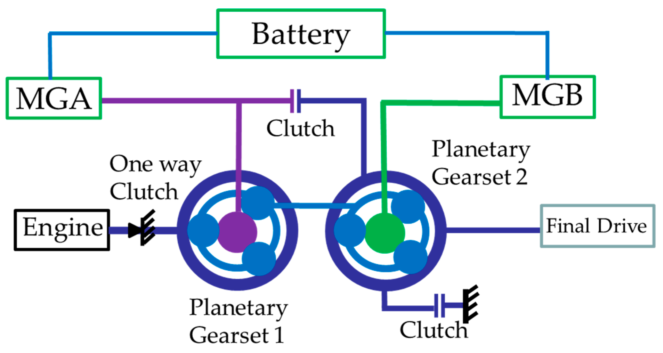
The AMBER software, version 2021 developed by Argonne National Laboratory, Chicago, USA has a vehicle model similar to the second-generation Chevrolet Volt produced by General Motors. This model was employed to validate the presented algorithms and understand the benefits, regenerative braking, and vehicle energy losses. The vehicle’s name in AMBER is Extended Range Electric Vehicle Midsize Voltec 2nd Generation. Figure 9 shows the powertrain of Volt Gen II. Volt Gen II is a PHEV with multiple modes of operation. The Volt Gen II powertrain is made up of one engine and two electric motors, a battery with power electronics, two planetary gear trains, and three clutches. The multiple modes of the powertrain are classified as electric vehicle (EV) mode and extended range mode (ER). Different powertrain modes are achieved by connecting three clutches, two electric motors, and an engine in distinct combinations. The simulation to generate the optimal velocity profiles were in MATLAB and SIMULINK, version 2020a, developed by MathWorks Inc., Natick, Massachusetts, USA. The test cases with different input values and combinations for variables were used to simulate the algorithm with the MPC optimization model, which output the velocity profile. The generated velocity profiles were executed in AMBER software to compute the vehicle outputs.

3.1. Validation for the Combination of Single and Multiple Phase Scenarios

Within this section, predictive velocity control to pass through the traffic intersection is tested using scenarios that take the uncertainties into consideration. As described in the signal timing plan manual [34], a framework was utilized for the traffic signal plan development and software to execute the plans. These uncertainties were due to the dynamic count of pedestrians waiting to cross, vehicles in the queue for a left turn, and the traffic flow rate for the lane in consideration. There were also some static causes of uncertainties, such as the traffic intersection proximity to a school, hospital, or shopping center. Such infrastructure can require more customization of the timing plans. The traffic also varies considerably, depending on whether the day is a weekday or a weekend. Not only phase duration but also the cycle duration can change based on the day and changing traffic conditions. These variables can make the estimation of the residual time of the phase decrease as well as increase during the active phase based on the transitory conditions of the traffic intersection. All these contributors make estimating the residual end time complex and challenging.

3.1.1. Design and Methodology for Generating Randomized End of Phase Time Estimations for Test Cases

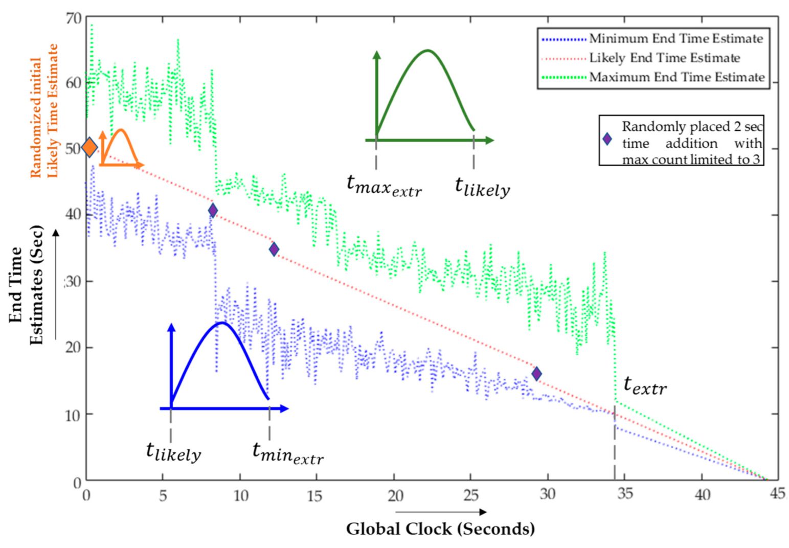
In this paper, the scope is to develop and verify an algorithm for vehicle velocity control considering the broadcasted SPaT messages from the traffic intersection, assuming that the accuracy is reasonable and as per the SAE J2735 [8]. The estimation of the major parameters in the SPaT messages, including the likely end time, the maximum end time, and the minimum end time, is discussed in this section. Figure 10 shows the estimation of these three parameters based on

Table 1. Predictive Velocity Control End Time Estimate Matrix.

Parameters		Road Function Classification [35]
		Major Arterial (>40 mph)		Major Arterial (<40 mph)	Minor Arterial
Speed Groups (mph)		55–50	45–40	40–35	35–30
Phase Duration	$t_{likel{y}_{in}}$	70–40		60–40	50–30
	$t_{{max}_{extr}}$	70		60	50
	$t_{{min}_{extr}}$	10		7	4
Minimum distance between intersections		0.5 mile (~805 m)			0.25 mile (~402 m)

and

Table 2. Upper and lower limit bounds for estimating the maximum and minimum end time.

Speed Groups	Time (s)
	Likely End Time $\left({\mathit{t}}_{\mathit{l}\mathit{i}\mathit{k}\mathit{e}\mathit{l}\mathit{y}}\right)$	$\mathbf{Upper} \mathbf{Bound} \mathbf{for} \mathbf{Maximum} \mathbf{Distribution} \left({\mathit{t}}_{{\mathit{m}\mathit{a}\mathit{x}}_{\mathit{U}\mathit{B}}}\right)$	$\mathbf{Lower} \mathbf{Bound} \mathbf{for} \mathbf{Minimum} \mathbf{Distribution} \left({\mathit{t}}_{{\mathit{m}\mathit{i}\mathit{n}}_{\mathit{L}\mathit{B}}}\right)$
(55–50) (45–40)	$<$$70 \mathrm{and} \ge$40	70	30
	$<$$40 \mathrm{and} \ge$30	50	10
	$<$$30 \mathrm{and} \ge$10	40	10
(40–35)	$<$$60 \mathrm{and} \ge$40	60	30
	$<$$40 \mathrm{and} \ge$30	50	7
	$<$$30 \mathrm{and} \ge$7	40	7
(35–30)	$<$$50 \mathrm{and} \ge$30	50	20
	$<$$30 \mathrm{and} \ge$20	40	4
	$<20$$\mathrm{and} \ge$4	30	4

. Table 1 gives information about green phase duration limits for different speed zones of roads. The likely end ($t_{likely})$ is initialized randomly using a normal distribution defined by the “Initialization range of $t_{likely}$” row in Table 1, denoted as $t_{likel{y}_{in}}$. The mean and standard deviation of the normal are defined by Equations (21) and (22). For the speed groups 55–50 mph and 45–40 mph, the upper bound and the lower bound of the initialization range of $t_{likely}$ were 70 s and 40 s, respectively. As a result, the mean of the normal distribution was as per Equation (21) with mean 55 s, i.e., $\frac{70+40}{2}$. The standard deviation was 3.75 $\left(\frac{70-40}{8}\right)$ as per Equation (22). The randomization was implemented using the ‘randn’ command in MATLAB/SIMULINK, as per Equation (23).

$$mean=\frac{upper limit+lower limit}{2}$$

(21)

$$standard deviation=\frac{upper limit-lower limit}{8}$$

(22)

$$Random number=(standard deviation\times randn\left(\mathrm{1,1}\right)+mean)$$

(23)

Once the $t_{likely}$ is initialized, the likely end time is linearly decayed, as shown in Figure 10. There are two types of disturbances: random decay and random increase. The random increase/random decrease of 2 s allowed in the $t_{likely}$ is allowed to emulate events such as more pedestrians waiting to cross than average and vehicle flow rate change. The maximum number of random increases and decreases was limited to 3 in this study, which represented 10% of the 60 s phase, to consider uncertainties and trust in the timing plans of the traffic intersections. Figure 10 shows a pictorial representation of the end of the phase time estimations over the total phase duration. The choice of adding the random increase or decrease of $t_{likely}$ was used to define different test cases. Two categories of test cases are defined in this study. In the first category, the likely end time linearly decreases and may have sudden increases of 2 s randomly, as shown in Figure 10. In the second category, the likely end time can decrease as well as randomly decrease in steps of 2 s during the active phase.

The distances for the phase end time estimation for different speed groups are defined in Table 1. Although DSRC only has a range of 300 m, cellular communication can broadcast to a wider range. We considered 805 m (0.5 miles) for speeds greater than 40 mph and 402 m (0.25 mile) for speeds less than 35 mph, which was shared in [34] and considered to be more than enough to plan for driving through the traffic intersection or coming to a stop. For every additional actuation by the detector/s, a typical 2 s extension was carried out for the current phase.

The estimation of the maximum end time $\left(t_{max}\right)$ and minimum end time $(t_{min}$) included two stages. In the first stage, the values of $t_{likely}$ were within the ranges in Table 2. In this stage, the upper bound and the lower bound to define the normal distribution of the maximum end time were the ‘Upper bound for maximum distribution’ $\left(t_{{max}_{UB}}\right)$ and the ‘Likely end time’ $(t_{likely}$) in Table 2. The upper bound and the lower bound to define the normal distribution of the minimum end time were the ‘Likely end time’ $\left(t_{likely}\right)$ and the ‘Lower bound for minimum distribution’ $({t_{min}}_{LB}$). At every 0.1 s instance, the maximum end time and the minimum end time were generated based on the corresponding normal distributions as per Equations (21)–(23). The second stage started when the likely time reached the lowest value of the speed group $(t_{likely}=t_{extr})$, as shown in Figure 10, which in the case of speed groups of 55–50 mph and 45–40 mph was $t_{extr}$ = 10 s. In the second stage, the maximum end time was estimated as 1.2 times the likely end time, and the minimum end time was estimated as 0.8 times the likely end time.

3.1.2. Tests, Results, and Discussion

Based on the details shared in the previous subsection, the test cases for validation are given below. Different scenarios were simulated to observe the algorithm’s behavior, and energy results are compared with the baseline.

Green Phase Throughout

Based on the details shared in the previous subsection, the test cases are listed for the validation. For each test case, the distance to be traveled is listed in Table 1. The initial velocity of the vehicle was randomized considering the uniform distribution within the speed group limit. For example, if the speed group was 55–50 mph, then the upper limit was 55 mph and the lower limit was 50 mph. The uniform distribution was implemented using ‘rand’ in MATLAB/SIMULINK. Random initial velocity generation is defined in Equation (24).

$$Random initial velocity=(upper bound-lower bound)\times rand\left(\mathrm{1,1}\right)+lower bound$$

(24)

The generated time estimate cycle was inputted into the optimization SIMULINK model to generate the reference velocity trace for the predictive velocity control. The MPC controller outputted the control actions to track the reference velocity profile. These control actions were used to calculate the actual vehicle velocity and recorder, which was inputted into the AMBER/AUTONOMIE Voltec Gen II model to determine the energy consumption numbers. The parameters were kept as the default except for the initial SOC. The road load co-efficients were from the EPA [36]. The initial SOC was considered to be 70%.

Table 3. Parameter Values for Validation.

Parameter	Values	Unit
Mass of Vehicle	1748	kg
$f_0$	120.55	N
$f_1$	2.1624	N/m/s
$f_2$	0.34707	$\mathrm{N}/\mathrm{m}/{\mathrm{s}}^2$
$g$	9.81	$\mathrm{m}/{\mathrm{s}}^2$
$\mathrm{Prediction} \mathrm{horizon} t_c$	10	s

shares the vehicle parameters for the simulation.

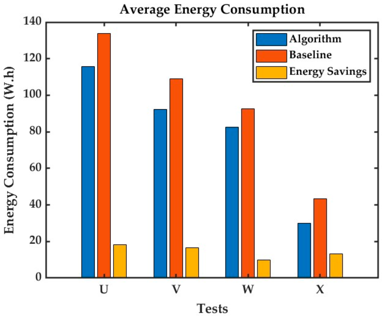
Figure 11 shows the energy consumption of each test case and the corresponding sub-tests in the same sequence, as described in

Table 4. Test Cases for the Validation of the Green Phase.

Speed Group	Tests		Initial Velocity (mph)	Initialized Green Phase Duration (s)
	Number	Disturbance Type
55–50	U1	Random Increase	52.1	54.2
	U2		54	50.7
	U3		53.6	51.8
45–40	V1	Random Decay	44.0	65.5
	V2		43.2	55.3
	V3		42.2	57.4
40–35	W1	Random Increase	37.4	52.7
	W2		38.2	51.2
	W3		35.8	50.7
35–30	X1	Random Decay	34.8	38.3
	X2		33.5	42.2
	X3		32.5	42.9

. The test results show that the algorithm helped to pass the intersection in all cases discussed. The energy consumption was compared to the baseline, which was the constant velocity followed throughout the distance and was same as the initial velocity.

Multiple Phase Scenarios (Vehicle May Stop or Decelerate Partially)

Additional scenarios were designed to observe the algorithm performance when a vehicle may need to stop or decelerate partially.

Table 5. Time Cycle Information for Imminent Stop Due to Longer Red Phase and Partial Green Phase.

Cycle	Phase	Duration (s)	Disturbances	Phase	Duration (s)	Disturbances	Disturbance Type
S.1	Green	20	2	Red	30	1	Random Decay
S.2		15	1		20	1
S.3		20	2		30	1	Random Increase
S.4		15	1		15	1

lists the test scenarios when a vehicle must stop. Table 8 lists the test scenarios when a vehicle may have to partially decelerate to pass the traffic intersection. Cycles S.1 and P.1 and S.3 and P.3 were used for testing the speed group of 55–50 mph. Cycles S.2 and P.2 and S.4 and P.4 were used for testing the speed group of 35–30 mph, as shown in

Table 6. Baseline for Multiple Phase Test Cycles.

Cycle	Speed Limit/Initial Velocity	Deceleration Distance Feet (Meters)
S/P.1 and S/P.3	55 mph	445 (135.6)
S/P.2 and S/P.4	35 mph	285 (86.8)

. The initial velocity for the simulation model was the speed limit of the group, e.g., 55 mph for the speed group 55–50 mph.

The baseline for these tests considered the initial velocity as the speed limit. The vehicle was driven at the initial velocity for all of the time before deceleration. The deceleration started at the distance interpreted from [34] and is listed in Table 6. For the test cycles in Table 5, the deceleration rate of the baseline was calculated by Equation (25) when the vehicle reached this distance. The final velocity was considered as zero.

$$Deceleration rate=\frac{Final Velocit{y}^2-Current Velocit{y}^2}{2\times Distance}$$

(25)

Table 7. Results for Imminent Stop Due to Red Phase.

Cycles	Energy Consumption (W.h)		Energy Gain (W.h)
	Algorithm	Baseline
S.1	−23.7	−11.6	12.1
S.2	−13.8	−11.7	2.1
S.3	−23.3	−11.6	11.7
S.4	−13.1	−11.7	1.4

shows the energy consumption results for the tests. Negative energy consumption was due to the regeneration energy being greater than the energy consumption during cruising in the respective velocity profile. For the overall task, the algorithm was able to use less energy to travel the same distance than the baseline.

For the test cycles in

Table 8. Time Cycle Information for Multiple Phases.

Cycle	Phase	Duration (s)	Disturbances	Phase	Duration (s)	Disturbances	Phase	Duration (s)	Disturbances	Disturbance Type
P.1	Green	30	2	Red	10	1	Green	65	3	Random Decay
P.2		20	1		10	1		50	2
P.3		20	2		10	1		65	3	Random Increase
P.4		18	1		4	0		50	3

where the vehicle decelerated partially and as the phase turned green, allowing the vehicle to pass through the intersection. Multiple phase test scenarios’ details are provided in

Table 9. Test results for Multiple Phase Scenarios.

Cycles	Energy Consumption (W.h)		Energy Gain (W.h)
	Algorithm	Baseline
P.1	34.0	38.2	4.2
P.2	16.6	18.3	1.7
P.3	−13.0	11.2	24.2
P.4	29.2	46.5	17.4

. The cycles P.1 and P.2 were random decay disturbances, and the remaining were random increase disturbances. The baseline definition was the same as discussed before. If acceleration was required, the acceleration rate was $2 \mathrm{m}/{\mathrm{s}}^2$.

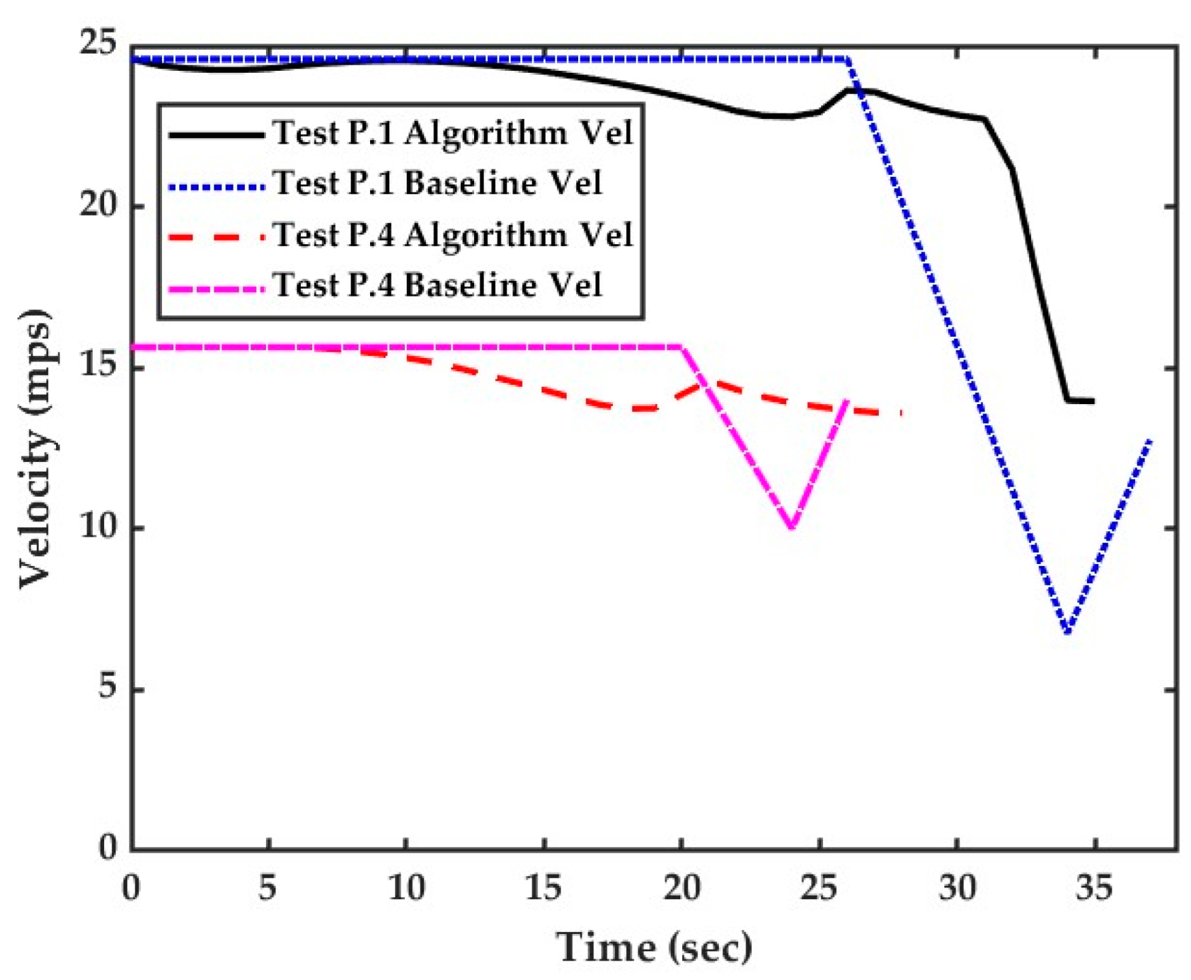
The reason for low as well as negative energy consumption was the regeneration being part of the energy consumption for the test cases. The test cycle P.1 had random decay disturbances with an initial velocity of 55 mph. The first phase in the cycle was green, and had a net duration of 26 s. The second phase in the same cycle is red, with a net duration of 8 s. The third phase was green again. As shown in Figure 12, the predictive vehicle velocity control algorithm made the vehicle gradually decelerate as compared to the baseline velocity profile. The baseline profile went to a lower velocity in comparison. When the phase changed to green, the deceleration was arrested. Additionally, the vehicle travelled the residual distance. The baseline profile decided to decelerate till the end of the red phase, and then accelerated to reach the traffic intersection.

If we consider test P.4, the cycle had a random increase in the type of disturbances. The first phase was green with a net duration of 20 s. The second phase was red, which had a duration of 4 s without any disturbance. The third phase was green again. The predictive vehicle velocity profile made the vehicle slow a bit for the small red phase duration and continue to pass the traffic intersection. However, the baseline profile decelerated to a much lower velocity and accelerated to travel the residual distance.

3.2. Validation for Eco-Stopping

In this section, the eco-stopping algorithm is validated using multiple scenarios. We had four test cases wherein the input was the initial vehicle velocity and the distance of the vehicle to the stop line, as shown in

Table 10. Eco-stopping Test Cases Details.

Test No.	Initial Velocity (mph)	Distance (Meters)
Test A	70.7	587.6
Test B	51.6	211.9
Test C	44.9	128.4
Test D	34.6	75.4

. The deceleration speed and distance values were taken from the US06 drive cycle. The deceleration profile segments of the US06 drive cycle were also treated as the baseline to measure the improvements. This was undertaken to simulate the condition for stop signs. The initial SOC value was 70%. The values of weighting factor ${\beta }_1$ = 1 and ${\beta }_2$ = $\frac{total distance}{initial velocity}$. This made the tuning factors automated based on the initial velocity and the amount of distance to be covered to stop at the designated spot.

The eco-stopping control actions generated with input as the given target distance and the initial velocity were recorded in Simulink. These control actions were integrated to find the velocity profile. The recorded velocity profile was then fed into the AMBER/Autonomie software to calculate the energy saved by the eco-stopping algorithm. The vehicle parameters were the same as in Table 3.

Table 11. Regenerative Energy Improvement Details.

Test No.	Regeneration Energy (W.h)
	Eco-Stopping	Baseline	Improvement
Test A	160.2	159.2	0.9%
Test B	101.1	99.6	1.5%
Test C	78.1	77.5	0.8%
Test D	46	45.8	0.4%

shows the energy regenerated back into the battery for each test run. The eco-stopping algorithm could maximize the regeneration energy. The percentage improvements ranged from 1.5% on the higher side to 0.4% on the lower side.

Table 12. Mechanical Brake Energy Gains.

Test No.	Mechanical Brake Energy (W.h)
	Eco-Stopping	Baseline	Improvement
Test A	31.8	32.5	0.7
Test B	21	22.2	1.2
Test C	17.3	17.8	0.5
Test D	11.4	11.9	0.5

had mechanical brake energy efficiency improvements. Equation (26) shows the calculation for Mechanical Brake Energy (MBE) from the simulation data. The eco-stopping algorithm could reduce the mechanical brake application, which contributed to energy regeneration.

$$MBE=Total Brake Energy-Regen Energy$$

(26)

Figure 13 shows the velocity and distance plots for four test cases. For each test case, the velocity profile could decelerate to zero velocity and stop at the designated stop spot. The distance was in a decaying state as it neared the stop spot.

Figure 14 shows the comparison of the regen power and brake power for the baseline and eco-stopping algorithm in Test B. It can be observed that the area covered by the regen power curve of the eco-stopping algorithm was larger than the area covered by the baseline regen power curve. The velocity profile generated by the eco-stopping helped to capture more energy as a result. The mechanical brake was utilized multiple times with the baseline velocity, while in the case of the eco-stopping velocity profile the brake was applied only once, at a lower speed where the opportunity to regenerate was also less.

4. Conclusions and Future Work

The paper presents optimal algorithms for a vehicle to pass through a semi-actuated/actuated traffic intersection or to maximize energy regeneration in case of an eminent stop and slow down to pass through a green phase. The algorithms were validated using the second-generation GM Volt model in AMBER/AUTONOMIE software developed by the Argonne National Laboratory. The presented methods can be applicable to different types of vehicles/powertrains with knowledge of the system design details.

Firstly, the predictive vehicle velocity control algorithm can handle the randomness of the end-of-phase-duration time estimations. Multiple test cases which incorporate randomness in the end-of-phase-duration estimations were employed to check the performance of the control algorithms. The proposed algorithms can show an improvement compared to the baseline. The algorithm can carry out vehicle velocity control in a better way to reduce energy consumption in the case of an imminent stop. In the case of multiple phase changes, the vehicle can slow down to reach the traffic intersection in a more energy efficient manner.

Secondly, the eco-stopping algorithm in a standalone manner can create more regeneration for the same distance and initial velocity in the deceleration sections of the US06 drive cycle. The vehicle was able to stop at the stop line, thus validating the algorithm’s suitability to come to zero velocity at the stop sign.

For future scope, as more real-world historical data of SPaT message becomes accessible, the control algorithm can be improved based on the probability density function of the available real-world data.

References

1. U.S. Energy Information Administration. Available online: https://www.eia.gov/ (accessed on 1 August 2019).
2. Utriainen, R.; Pöllänen, M. The Needed Features of Connected and Automated Vehicles to Prevent Passenger Car Crashes Caused by Driving Errors. Future Transp. 2021, 1, 370–386. [Google Scholar] [CrossRef]
3. Karbasi, A.; O′Hern, S. Investigating the Impact of Connected and Automated Vehicles on Signalized and Unsignalized Intersections Safety in Mixed Traffic. Future Transp. 2022, 2, 24–40. [Google Scholar] [CrossRef]
4. Nazari Enjedani, S.; Khanal, M. Development of a Turning Movement Estimator Using CV Data. Future Transp. 2023, 3, 349–367. [Google Scholar] [CrossRef]
5. Abduljabbar, R.; Dia, H.; Tsai, P.-W.; Liyanage, S. Short-Term Traffic Forecasting: An LSTM Network for Spatial-Temporal Speed Prediction. Future Transp. 2021, 1, 21–37. [Google Scholar] [CrossRef]
6. Chen, J.; Qian, L.J.; Xuan, L. Cooperative control of connected hybrid electric vehicles and traffic signals at isolated intersections. IET Intell. Transp. Syst. 2021, 14, 1903–1912. [Google Scholar] [CrossRef]
7. Chen, B. Intelligent Control to Reduce Vehicle Energy Consumption and Greenhouse Gas Emissions; Spring Nature: Basel, Switzerland, 2022. [Google Scholar] [CrossRef]
8. SAE. Dedicated Short Range Communications (DSRC) Message Set Dictionary; SAE International: Warrendale, PA, USA, 2016; Volume 359. [Google Scholar] [CrossRef]
9. Asadi, B.; Vahidi, A. Predictive Cruise Control: Utilizing Upcoming Traffic Signal Information for Improving Fuel Economy and Reducing Trip Time. IEEE Trans. Control. Syst. Technol. 2011, 19, 707–714. [Google Scholar] [CrossRef]
10. Mahler, G.; Vahidi, A. An Optimal Velocity-Planning Scheme for Vehicle Energy Efficiency Through Probabilistic Prediction of Traffic-Signal Timing. IEEE Trans. Intell. Transp. Syst. 2014, 15, 2516–2523. [Google Scholar] [CrossRef]
11. Ibrahim, S.; Kalathil, D.; Sanchez, R.O.; Varaiya, P. Estimating Phase Duration for SPaT Messages. IEEE Trans. Intell. Transp. Syst. 2019, 20, 2668–2676. [Google Scholar] [CrossRef]
12. Mathew, J.; Li, H.; Bullock, D.M. Using Stochastic Variation of Cyclic Green Distributions to Populate SAE J2735 Message Confidence Values along a Signalized Corridor. Transp. Res. Rec. J. Transp. Res. Board 2020, 2674, 426–437. [Google Scholar] [CrossRef]
13. Hao, P.; Wu, G.; Boriboonsomsin, K.; Barth, M.J. Eco-Approach and Departure (EAD) Application for Actuated Signals in Real-World Traffic. IEEE Trans. Intell. Transp. Syst. 2019, 20, 30–40. [Google Scholar] [CrossRef]
14. Sun, C.; Gaunetti, J.; Borrelli, F.; Moura, S. Robust Eco-Driving Control of Autonomous Vehicles Connected to Traffic Lights. arXiv 2019, arXiv:1802.05815. [Google Scholar]
15. Rostami-Shahrbabaki, M.; Niels, T.; Hamzehi, S.; Bogenberger, K. An Independent Trajectory Advisory System in a Mixed-Traffic Condition: A Reinforcement Learning-Based Approach. IFAC-PapersOnLine 2020, 53, 15667–15673. [Google Scholar] [CrossRef]
16. Zhang, R.; Yao, E. Eco-driving at signalised intersections for electric vehicles. IET Intell. Transp. Syst. 2015, 9, 488–497. [Google Scholar] [CrossRef]
17. Qiu, L.; Qian, L.; Zomorodi, H.; Pisu, P. Global optimal energy management control strategies for connected four-wheel-drive hybrid electric vehicles. IET Intell. Transp. Syst. 2017, 11, 264–272. [Google Scholar] [CrossRef]
18. Bhat, P.K.; Oncken, J.; Yadav, R.; Chen, B.; Shahbakhti, M.; Robinette, D. Generation of Optimal Velocity Trajectory for Real-Time Predictive Control of a Multi-Mode PHEV. In Proceedings of the 2019 IEEE 90th Vehicular Technology Conference (VTC2019-Fall), Honolulu, HI, USA, 22–25 September 2019; pp. 1–5. [Google Scholar]
19. Oncken, J.; Orlando, J.; Bhat, P.K.; Narodzonek, B.; Morgan, C.; Robinette, D.; Chen, B.; Naber, J. A Connected Controls and Optimization System for Vehicle Dynamics and Powertrain Operation on a Light-Duty Plug-In Multi-Mode Hybrid Electric Vehicle. In Proceedings of the SAE Technical Paper Series, Detroit, MI, USA, 21–23 April 2020. [Google Scholar]
20. Robinette, D.; Chen, B.; Bhat, P.; Oncken, J.; Orlando, J.; Rama, N. Leveraging Connectivity and Automation to Improve Propulsion System Energy Sufficiency. In Proceedings of the CTI SYMPOSIUM 2018: 17th International Congress and Expo, Berlin, Germany, 3–6 December 2018; pp. 300–309. [Google Scholar]
21. Barik, B.; Bhat, P.K.; Oncken, J.; Chen, B.; Orlando, J.; Robinette, D. Optimal velocity prediction for fuel economy improvement of connected vehicles. IET Intell. Transp. Syst. 2018, 12, 1329–1335. [Google Scholar] [CrossRef]
22. Bhat, P.K. Study of Optimal Velocity Trajectory for Real-Time Predictive Control of a Multi-Mode PHEV; Michigan Technological University: Houghton, MI, USA, 2019. [Google Scholar] [CrossRef]
23. Oncken, J.; Chen, B. Real-Time Model Predictive Powertrain Control for a Connected Plug-In Hybrid Electric Vehicle. IEEE Trans. Veh. Technol. 2020, 69, 8420–8432. [Google Scholar] [CrossRef]
24. Zhang, X.; Li, X.; Zhang, Z. Data-Driven-Based Eco Approach for Connected and Automated Articulated Trucks in the Space Domain. Sustainability 2023, 15, 1229. [Google Scholar] [CrossRef]
25. Wen, Y.; Wang, Y.; Zhang, Z.; Wu, J.; Zhong, L.; Papageorgiou, M.; Zheng, P. Effects of Connected Autonomous Vehicles on the Energy Performance of Signal-Controlled Junctions. Sustainability 2023, 15, 5672. [Google Scholar] [CrossRef]
26. Wu, Z.; Bhat, P.K.; Chen, B. Optimal Configuration of Extreme Fast Charging Stations Integrated with Energy Storage System and Photovoltaic Panels in Distribution Networks. Energies 2023, 16, 2385. [Google Scholar] [CrossRef]
27. Treiber, M.; Kesting, A. Traffic Flow Dynamics. In Traffic Flow Dynamics; Springer: Berlin/Heidelberg, Germany, 2013; p. 190. [Google Scholar]
28. Conlon, B.M.; Blohm, T.; Harpster, M.; Holmes, A.; Palardy, M.; Tarnowsky, S.; Zhou, L. The Next Generation “Voltec” Extended Range EV Propulsion System. SAE Int. J. Altern. Powertrains 2015, 4, 248–259. [Google Scholar] [CrossRef]
29. Ferreau, H.J.; Bock, H.G.; Diehl, M. An online active set strategy to overcome the limitations of explicit MPC. Int. J. Robust Nonlinear Control. 2008, 18, 816–830. [Google Scholar] [CrossRef]
30. Ferreau, H.J.; Kirches, C.; Potschka, A.; Bock, H.G.; Diehl, M. qpOASES: A parametric active-set algorithm for quadratic programming. Math. Program. Comput. 2014, 6, 327–363. [Google Scholar] [CrossRef]
31. Houska, B.; Ferreau, H.J.; Diehl, M. ACADO toolkit-An open-source framework for automatic control and dynamic optimization. Optim. Contr. Appl. Met. 2011, 32, 298–312. [Google Scholar] [CrossRef]
32. Rousseau, A.; Pagerit, S.; DeLaughter; Juskiewicz, M.; Sharer, P.; Vijayagopal, R. AMBER: A New Architecture for Flexible MBSE Workflows. In Proceedings of the IEEE VPPC 2017, Belfort, France, 14–17 December 2017. [Google Scholar]
33. Autonomie, Rev16; Argonne National Laboratory: Chicago, IL, USA, 2021.
34. Urbanik, T.; Tanaka, A.; Lozner, B.; Lindstrom, E.; Lee, K.; Quayle, S.; Beaird, S.; Tsoi, S.; Ryus, P.; Gettman, D.; et al. Signal Timing Manual, 2nd ed.; Transportation Research Board: Washington, DC, USA, 2015. [Google Scholar]
35. Federal Highway Administration. Road Function Classification. 2000. Available online: https://safety.fhwa.dot.gov/speedmgt/data_facts/docs/rd_func_class_1_42.pdf (accessed on 15 June 2022).
36. EPA. Data on Cars Used for Testing Fuel Economy. Available online: https://www.epa.gov/compliance-and-fuel-economy-data/data-cars-used-testing-fuel-economy (accessed on 10 July 2022).
Figure 1. General Hierarchy of Control System for a Connected and Automated Vehicle Ecosystem.
Futuretransp 03 00038 g001
Figure 2. Velocity Profiling using SPaT information.
Futuretransp 03 00038 g002
Figure 3. Time estimates for phase duration.
Futuretransp 03 00038 g003
Figure 4. An overview of predictive velocity control at automated signalized intersections.
Futuretransp 03 00038 g004
Figure 5. Pseudo code for optimization feasibility.
Futuretransp 03 00038 g005
Figure 6. Pseudo code for selecting target velocity.
Futuretransp 03 00038 g006
Figure 7. Regeneration Paddle—Acceleration Data and Fit.
Futuretransp 03 00038 g007
Figure 8. Overall Architecture of Predictive Vehicle Control at Automated Signalized Intersections.
Futuretransp 03 00038 g008
Figure 9. GM Volt Gen II Powertrain Architecture.
Futuretransp 03 00038 g009
Figure 10. Estimation of End Time with reference to Table.
Futuretransp 03 00038 g010
Figure 11. Energy Consumption for Tests U, V, W, and X.
Futuretransp 03 00038 g011
Figure 12. Velocity Profile for Multiple Phase Change Scenarios.
Futuretransp 03 00038 g012
Figure 13. Velocity and Distance versus Time.
Futuretransp 03 00038 g013
Figure 14. Regen Power and Bake Power vs. Time.
Futuretransp 03 00038 g014