1. Introduction
Autonomous vehicles (AV) and connected autonomous vehicles (CAVs) are poised to change the way households and individuals own, drive, and operate their vehicles and how the transportation system performs and responds to traffic. Their introduction will potentially improve traffic safety [
1,
2], and roadway operation and capacities [
3,
4,
5]. AVs and CAVs have the potential to increase capacity in traffic streams by reducing vehicle headway, improving reaction times and sensitivity to changing traffic conditions, and promoting a more consistent and efficient flow of traffic. The hypothesis is that existing roadways may be better equipped to handle an increased proportion of AVs and CAVs compared to the exclusively traditional vehicles present today. Although there is an increasing amount of literature on autonomous vehicles, the relationship between penetration timelines and different mixes of AVs and CAVs has yet to be fully understood. Transportation planners must comprehend these impacts as they develop long-range transportation plans, which are commonly designed to forecast land use impacts on the transportation system for a period of up to 30 years into the future. These plans serve as a basis for making significant transportation system-wide investment decisions and require the development of models incorporating land use, transportation systems, and sociodemographic forecasts to predict their impact on travel demand and the transportation system. With the potential introduction of AVs and CAVs, planners are currently faced with the question of how these vehicles will impact roadways within the planning horizon (20–30 years from now) and how they should plan accordingly. As AVs and CAVs do not currently exist, this question is being addressed through simulation models that replicate their operations.
The problem addressed in this study is the lack of understanding of the impacts of AVs and CAVs on long-range transportation planning. Although studies have evaluated different technology mixes of AVs, CAVs, and traditional vehicles, they have not incorporated penetration and fleet timelines into the planning-level analysis. Transportation planning typically involves forecasting travel demand and its effects on the transportation system over a long-range period, which are then used to inform transportation system investment decisions. The literature has also not explored the proper calibration and validation process in oversaturated traffic conditions, where demand exceeds capacity and leads to heavy congestion and long queues. This type of traffic environment may have significant impacts on roadway capacity and deserves further investigation. With highway systems lasting 20 to 30 years, understanding the timeline-linked impacts of AVs and CAVs on the transportation system is crucial. Therefore, this study uses a simulation-based approach, incorporating AV/CAV operational and driving technologies and penetration forecasts, to address the gaps in the literature and provide important information for transportation planners to make informed decisions.
2. Background and Literature Review of AV/CAVS
AVs and CAVs are vehicles capable of performing driving functions, from assisting drivers with automatic cruise control and lane centering to fully driving the vehicle without any human intervention from start to finish. The concept of AVs/CAVs has been defined in various ways in the literature, based on the capabilities of the vehicles. For instance, the National Highway Traffic Safety Administration (NHTSA, 2016) categorizes AVs into six levels, based on the level of human intervention required in vehicle operation. Meanwhile, the Institute of Transportation Engineers (ITE, 2021) defines CAVs as having vehicle-to-vehicle (V2V), vehicle-to-infrastructure (V2I), and vehicle-to-mobile/smart device (V2X) connectivity via 5G.
The Coexist project (Coexist1.4, 2018) classifies AVs into three categories: cautious, normal, and all-knowing, with the latter being equivalent to a level 5 CAV from the NHTSA definition. However, the technologies and algorithms used in each class differ. For instance, an AV-normal vehicle can measure the distance and speed of other vehicles, slow down when its sensors detect blind spots, and avoid collisions, but it drives cautiously and leaves larger gaps in a traffic stream compared to traditional vehicles. On the other hand, CAVs can leave smaller gaps in a traffic stream, potentially increasing roadway capacities, as they incorporate V2X communication and more aggressive driving behavior. The impact of AVs/CAVs on highway capacity will be influenced by their driving behavior, particularly in oversaturated traffic conditions, and the level of penetration of these vehicles in the traffic stream along with traditional vehicles.
The gaps that these vehicles will leave in a traffic stream compared to traditional vehicles will play an important role in their highway capacity and operational impact. The impact becomes more pronounced under oversaturated traffic conditions, where traditional vehicles leave relatively smaller gaps and traffic is at stop-and-go speeds. The driving algorithms of AV-cautious vehicles may result in larger gaps in front of them compared to traditional vehicles, potentially reducing highway capacity. Conversely, CAVs have the potential to leave smaller gaps and increase roadway capacity. This issue is further complicated by the presence of AVs/CAVs at varying penetration levels and coexisting with traditional vehicles in the same traffic stream.
The market penetration of AV/CAVS will perhaps have the most significant capacity impact up until they reach critical mass in the vehicle fleet and in the amount of travel that occurs by them. Current research shows that AVs are expected to take longer to be accepted than other vehicle technologies [
6,
7]. Several factors including safety [
8], psychological [
9], trust [
10] and perceived usefulness/risk [
11]. These studies show that these factors will play an important role in the adoption cycles for AVs. Thus, our study uses the current state-of-the-art in future forecasts for AVs. These forecasts could change and have changed over the past several years. However, this research is developed to aid planners with accounting for AVs in their transportation plans. These plans are updated every five years in the U.S. and it will be appropriate to revisit AV forecasts periodically and adjust models accordingly. Therefore, significant capacity impacts may probably be seen 20 to 30 years from now. Regarding AV/CAV vehicle penetration, it is estimated that 50% of new vehicle sales will be AVs by 2045, and half of the fleets will be autonomous by 2060 [
12].
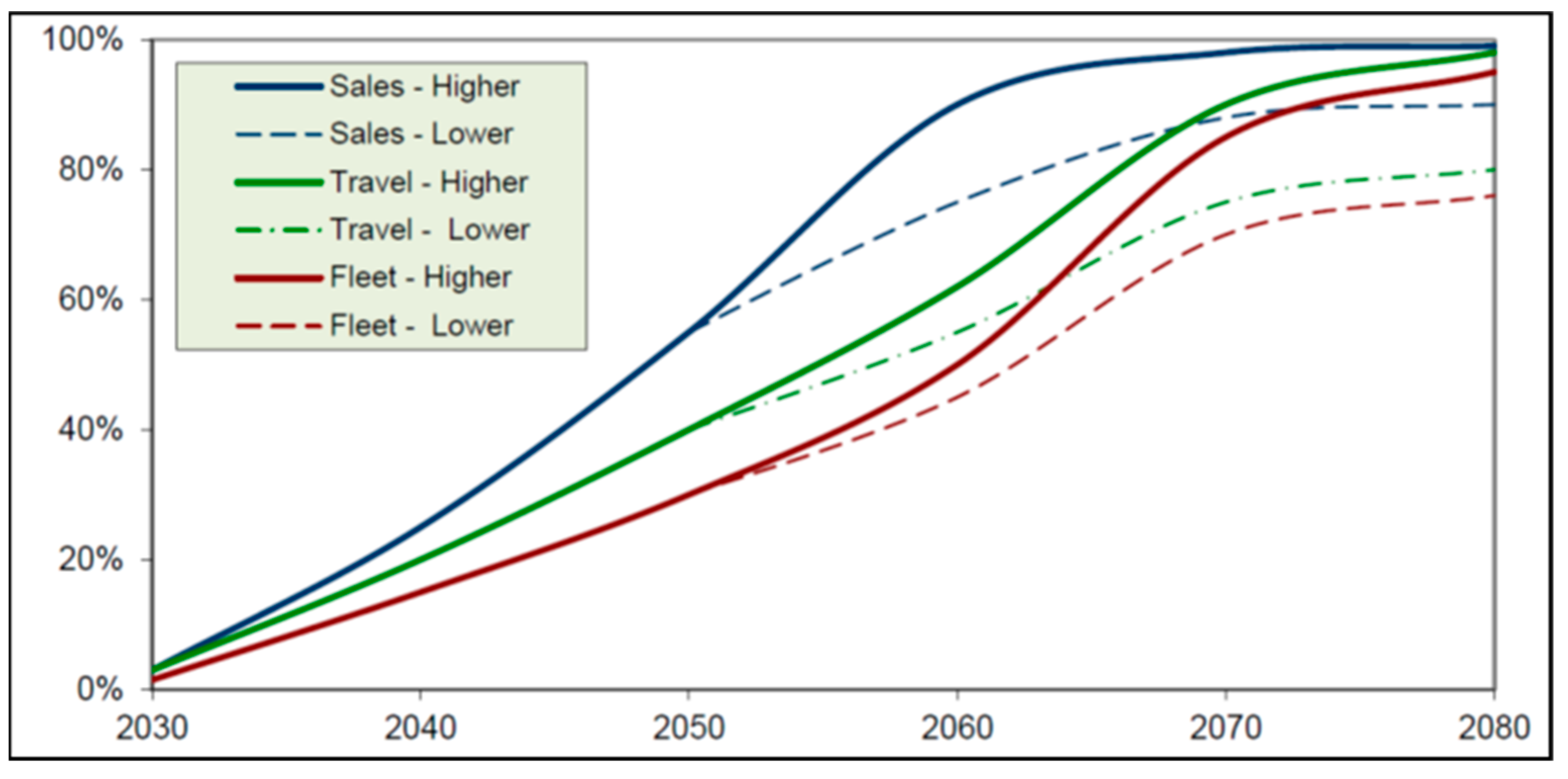
Figure 1 shows the forecasts of AV and CAV market penetration, travel, and fleet size over the next 60 years for potential worst and best cases [
12]. It shows that by 2050, which is the current long-range planning horizon year for metropolitan planning organizations in the U.S., travel by AVs/CAVs will be about 40% of total vehicle miles traveled. This is significant and will have different implications compared to the forecast year 2035 which is in the current mid-range planning horizon with about 15% penetration with mostly AV-cautious cars.
The effect is that transportation capacities will become fluid and change as AVs and CAVs change in the general vehicle population. For example, according to
Figure 1, significant benefits of AV/CAVS may only be realized after the year 2050. Since the planning horizon for most long-range transportation plans is 30 years in the U.S., it is possible that the full benefits will not materialize within the current long-range transportation plan horizons. In contrast, there are potentially negative impacts on capacity with lower penetrations and less aggressive technology. It is thus essential to correctly quantify the capacity impacts of AVs and CAVs to make optimal transportation system decisions over different planning time horizons. These impacts need to be investigated so that planners can make optimal decisions about their transportation system investments. Several studies have estimated the capacity impacts due to AVs and CAVs, with most showing improvements in capacities based on penetration rates, traffic conditions, and roadway types. Three main frameworks are used in the literature to evaluate these impacts, including mathematical formulations, simulation methods using synthetic data, and using real-world data to simulate these impacts.
A theoretical-mathematical formula was used to investigate the influence of vehicular technology on the car-following model [
13]. The results showed potential capacity improvements ranging from 20% to 50%. Another research found that AVs/CAVs decreased headway and at higher penetration levels increased capacity by up to 36% [
14,
15]. Mathematical models are good initial models that are incorporated into simulations that mimic real-world traffic behaviors and can be validated against real-world data.
Sensors and vehicle-to-vehicle (V2V) communication were used by [
16] to estimate the impacts of AVs. They found a 43% increase in capacity if all vehicles utilized sensors and V2V communication. An analytic and simulation-based approach was used to estimate the impacts of connection and automation [
17]. They showed that CAVs had better capacity impacts than AVs at the same penetration rate. The influence of Adaptive Cruise Control (ACC) and Cooperative Adaptive Cruise Control (CACC) on traffic flow was estimated in another study [
18]. This study showed that CACC stabilized and improved capacity better than ACC. This was achieved through platooning which had better capabilities to streamline traffic. These studies did not include mixed traffic scenarios which limit their applications by transportation planners.
Mixed traffic (Autonomous and regular vehicles) cooperative and opportunistic platooning schemes were analyzed using average platoon length and the capacity of a mixed-traffic freeway [
19]. The worst and best-case scenarios were considered for this study. Assuming a penetration rate of CAVs of 50% and using the most cautious possible platooning settings, a cooperative strategy could support 2806 vehicles per hour/lane. In contrast, an opportunistic strategy could support 2452 vehicles per hour/lane. This is a 31% and 14% increase over the previous maximum of 2142 vehicles per hour for a lane without platooning.
Penetration levels have been used in the literature to evaluate the impacts of AVs/CAVs. Capacity impacts for AVs/CAVs were evaluated using simulations on roundabouts [
20]. Their results showed that penetration rates were correlated to capacity enhancements. They created capacity adjustment factors for use with the Highway Capacity Manual (HCM) values. Another study considered a mixed scenario of CAVs using a modified MIXIC (a microscopic simulation software) car-following model, to analyze interstate capacity in mixed traffic situations [
21]. The results indicated a 28% increase in capacity owing to AVs and a 92% increase due to CAVs.
Other studies have also looked at different penetration levels and mixes of AVs/CAVs. A study worked on the potential impact of CAVs using different market penetration rates of 25%, 50%, 75%, and 100% to estimate the impacts of AVs [
22]. Their study showed that delays will decrease for all levels of penetrations of AVs. In another study [
23], the authors used different penetration rates of AVs to evaluate their impacts on roundabouts. The results also indicated that AV penetration levels will play a role in positively impacting transportation capacities.
Table 1 shows some key findings of the previous studies related to AV/CAV market penetration. However, these studies did not approach AV/CAV penetration from a long-range transportation planning perspective. Instead, they used fixed penetration rates which are important to consider in traffic operations. However, these studies do not provide the full picture for transportation planners to answer the AV/CAV impacts question based on their transportation plans which are typically time-based.
Moreover, in previous studies for capacity measurement of Basic Freeway Segment (BFS), Weaving, and Ramp junction, detector data were used to change the headway values for AV and CAV using a simulation model to estimate capacity [
34]. The authors used real-world point data to obtain the Wiedemann calibration parameters for the traditional vehicle, but not for the AV or the CAV. Instead, they utilized headway values of 0.9 for the AV and 0.6 for the CAV. Using point data was a shortcoming for current models that predict the impacts of AVs/CAVs. Point data may misrepresent a study section by not considering varying driver speeds and driver behaviors at different points in a roadway section. Using trajectory data rather than point data will improve the ability of models to predict real-world conditions correctly.
Calibration and validation play an essential role in microsimulation model development. Also, choosing drivers’ preferred speed distribution from unsaturated data is simple. Driver-selected speed distribution refers to driver-selected velocity in free-flow conditions on the freeway. Studies have used unsaturated to oversaturated traffic data with free-flow speed distribution [
35,
36,
37,
38]. However, a proper validation process is a shortcoming of those studies.
3. Problem Statement, Research Objective, and Research Contribution
Transportation planners are faced with the challenge of forecasting the impacts of AV and CAV technologies on the capacity of the transportation system. Although some studies have investigated the impacts of AVs and CAVs using various methods, including theoretical frameworks and simulation methods, there is a lack of models that enable planners to adequately forecast these impacts for different levels of AV/CAV penetration which also includes planning timeline horizons. Moreover, planners are constantly asking questions about the timing of AV/CAV penetration and their impacts on transportation planning over different time horizons. For example, how will AV/CAV technology impact capacity in 2040 as opposed to 2050? Without adequate tools to estimate the impacts of AVs/CAVs based on temporal-based technologies and their potential penetration levels, planners may overestimate or underestimate capacity impacts in long-range transportation plans. To address these gaps, this study simulated various penetration/mix levels of AVs, CAVs, and traditional vehicles for a basic freeway section using a mixed traffic simulation environment with state-of-the-art forecasts of AV/CAV penetration. By doing so, this study provides planners with new insights into the potential capacity impacts of AVs/CAVs for different planning horizons and penetration levels, thus aiding them in making informed decisions for future transportation investments.
The objective of this study was to estimate the capacity impacts of AVs/CAVs in oversaturated conditions with a mixed situation of traditional cars over different transportation planning horizons. Using a simulation-based approach that incorporates time-based AV/CAV penetration and technology predictions, we evaluated the capacity impacts for a basic freeway segment in oversaturated conditions. The main contributions of this study are twofold. First, we provide valuable information for transportation planners and decision-makers in making medium and long-term transportation decisions regarding the impact of AVs/CAVs on capacities over various planning horizons. Our study expands on the previous literature by incorporating time-based AV/CAV penetration and technology predictions to estimate the planning horizon of capacity impacts with mixed levels of AVs and CAVs over the next several decades. In addition, we provide a step-by-step process for estimating calibration parameters from trajectory data to use in microsimulation models. Second, our study contributes to the literature by addressing gaps in the current literature, specifically the lack of consideration for the stochastic effects of AV/CAV penetration on transportation planning efforts. The findings of this study provide important insights for transportation planners and decision-makers in developing effective and sustainable transportation plans, as well as for researchers and scholars in the field of transportation planning and engineering.
4. Materials and Methods
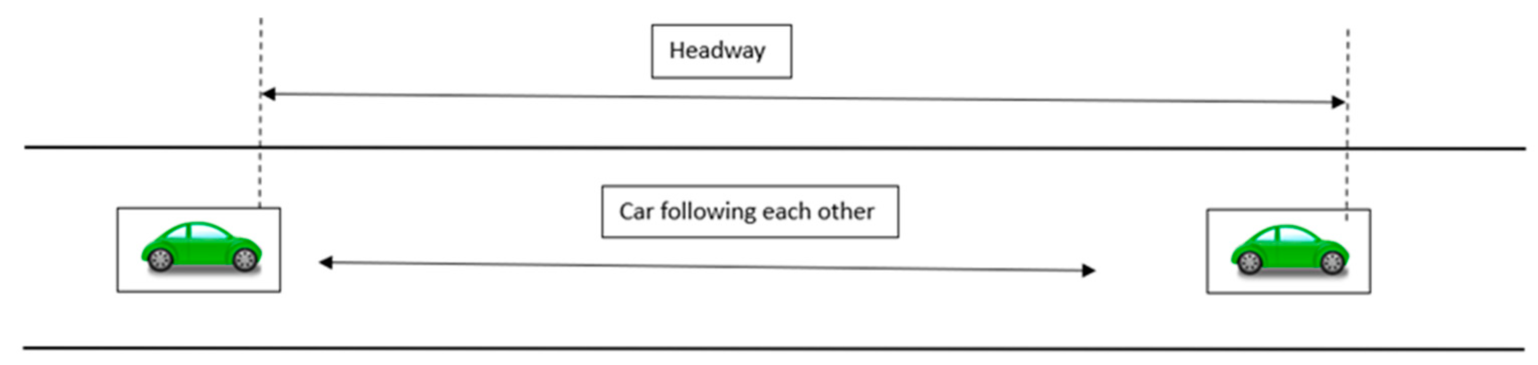
Microsimulation models are frequently used to estimate safety, capacity, and level of service impacts for various traffic conditions. These models use car-following models (CFMs) to replicate real-world driving behaviors in traffic. CFMs describe how vehicles follow each other in a continuous traffic flow and often contain driver behavior, vehicle features, and highway conditions and attributes. A comprehensive review of CFM methods can be found in [
25]. These models often contain driver behavior such as how aggressive drivers are, how much headway they give to vehicles in front of them in traffic, vehicle features, and highway conditions and attributes.
The methodology used in this research used vehicle behavior data from a real-world trajectory dataset to calibrate and validate a base model for saturated driving conditions. We then used AV/CAV car-following parameters from the Coexist project [
39] and time-based AV/CAV penetration data [
12], to develop several scenarios to evaluate the planning-level capacity impacts of AVs/CAVs. To achieve our objectives, we utilized microsimulation within the VISSIM software, using the Wiedemann car-following model. This model is a collision-free model that takes into account speed, space gap, time gap, and acceleration between two successive vehicles with four driving regimes: free flow, approaching, following, and braking. According to this model, a vehicle’s response is triggered by the difference in speed between the leading and trailing vehicles, such as acceleration or deceleration.
In the context of AV/CAV technology, microsimulation models can provide valuable insights into the potential effects of different AV/CAV technologies on transportation system capacities. By using real-world trajectory data to calibrate and validate the base model, researchers can ensure that the model reflects actual driving behaviors under different traffic conditions.
Furthermore, the use of AV/CAV car-following parameters from the Coexist project and time-based AV/CAV penetration data allows for the development of various scenarios to evaluate the planning-level capacity impacts of AVs/CAVs. By employing microsimulation inside the VISSIM software using the Wiedemann car-following model, researchers can simulate the behavior of all vehicles in a traffic stream, including AVs and CAVs, and evaluate their impact on traffic flow. This approach allows for a detailed evaluation of different AV/CAV technologies and their impact on traffic flow, making it a valuable tool for transportation planners and decision-makers.
The overall model structures deal with speed, distance, acceleration, and relative speed. The equations for diverse conditions, this model is designed to be accident-free as shown in
Figure 2.
4.1. Study Area Description and Data Collection
The next-generation simulation (NGSIM) data are an open data source developed by the FHWA [
40]. The data used for this study were collected on 15 June 2005, from 7.50 to 8.35 a.m. in US10 in Los Angeles, CA, from Lankershim Boulevard to Cahuenga Boulevard using video cameras mounted on top of 36-story buildings (
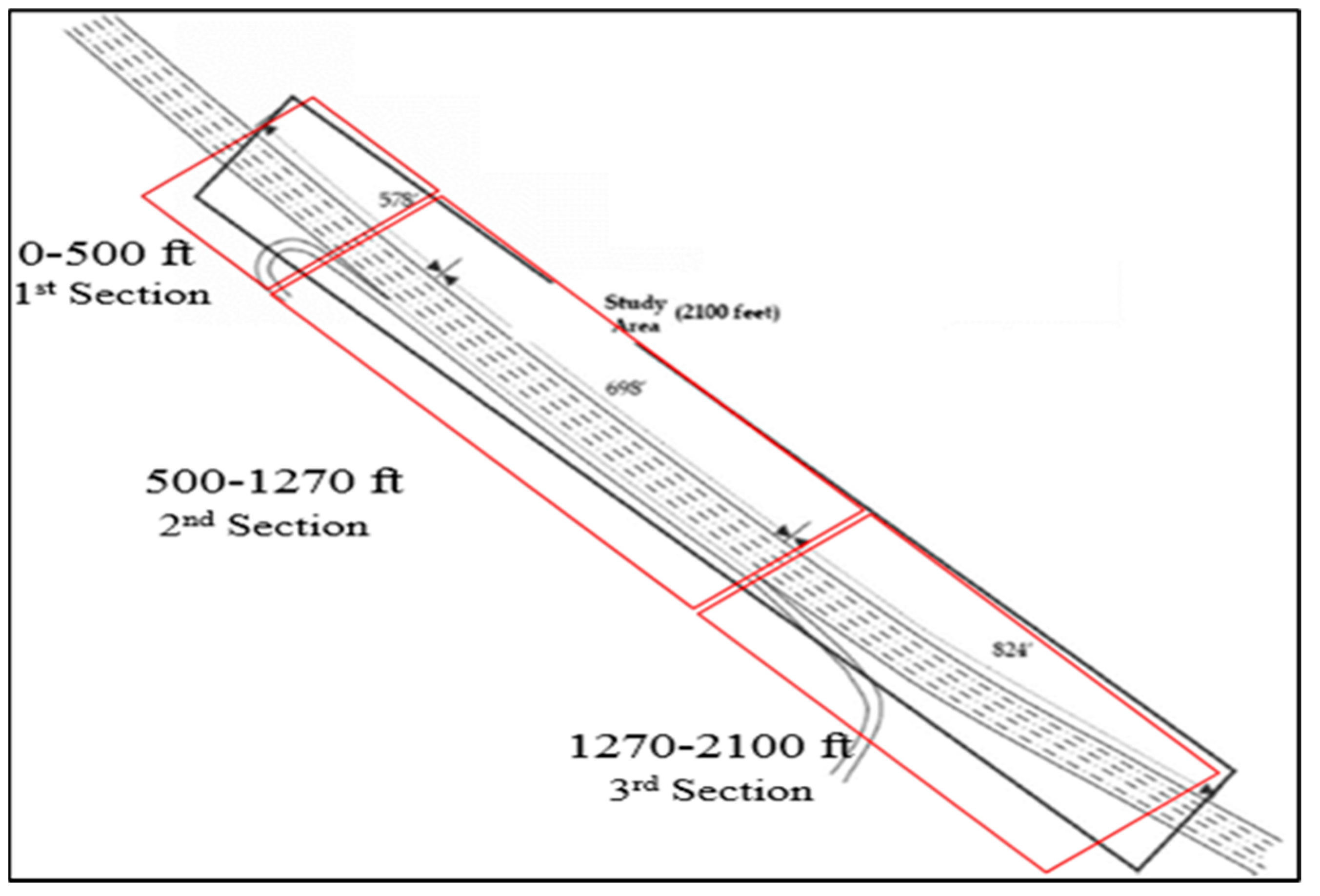
Figure 3). The length of the study section was 2100 feet with five main lanes, one auxiliary lane, one on-ramp, and one ramp. The complete vehicle trajectory was transcribed at a resolution of 10 frames per second. There are three classes of vehicles available in the dataset. Passenger cars, heavy vehicles, and motorcycles. Only passenger cars and heavy vehicles are used for this study due to the low number of motorcycles in the data. The study section had a posted speed of 55 mph.
The data were divided into 15 min time bins for estimating the different calibration components’ (CC) values due to different mean speeds at different intervals during the data collection period. The first 15 min of data showed that the lane space mean speeds (SMSs) were below 26.5 mph, indicating oversaturation conditions. The second 15 minutes’ mean speeds were lower than the first 15 min, also indicating over-saturated traffic conditions. This is expected especially in weaving sections where speeds can be lower due to merging traffic. The roadway section was divided into three sections for this reason. The start of the data collection point (0–500 ft) was defined as the first section, the next section (500–1270 ft was defined as the second section, and the section (1270–2100 ft) was defined as the third section as shown in
Figure 3.
4.2. Base Model Calibration
This study used VISSIM microsimulation software that needed calibration to match the transportation system and driver behavior on the roadways under study. The calibration started by estimating CC parameters for passenger cars and heavy vehicles, only for traditional vehicles. These parameters depicted driver behaviors and vehicle populations in a traffic flow. The CC parameters, such as space gap, time, relative velocity, and acceleration, indicated overall driver behavior for vehicles following each other. Calibration involved adjusting the CC parameters and comparing the simulated and observed output. In this study, we compared the simulated and observed mean speed (macro) and cumulative speed distribution (micro). The four leftmost lanes from 7.50–8.05 AM were used for basic freeway calibration. The CC values were calibrated based on vehicle type, as shown in
Figure 4 and
Figure 5. We used these methods to calibrate 10 CC parameter values for passenger cars and trucks:
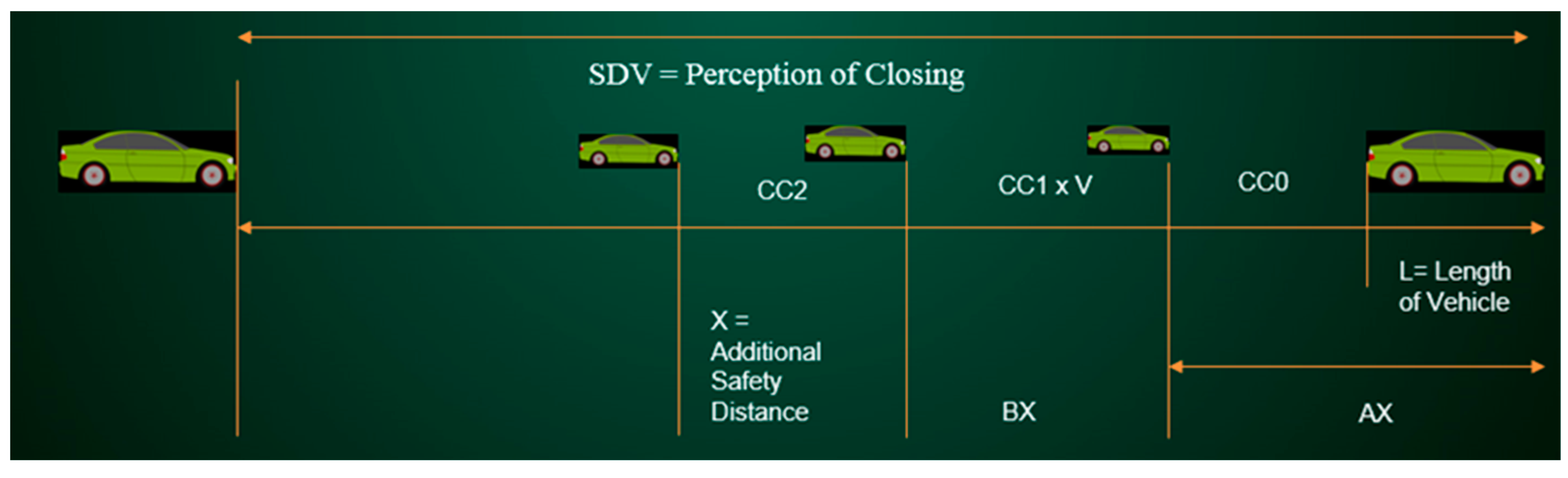
CC0 (space gap) is the distance the following vehicle keeps from the lead vehicle when stopped. It is the distance between the rear bumper of the front vehicle to the front bumper of the following vehicle when stopped. We calculated CC0 using vehicles with a 0–10 mph speed range (AX in
Figure 4) to represent stopped vehicles. The mode space headway value was estimated from NGSIM data, subtracting the average vehicle length. The average car length used was 14.5 ft and the heavy vehicle length was 32.5 ft.
CC1 (time gap) is the time gap between two consecutive vehicles in motion, after CC0. We estimated these values using speeds of more than 10 mph for the following vehicle in the dataset.
CC2-CC5 value were measured from the spacing vs relative velocity graphs shown in
Figure 5a.
Figure 5a is created from vehicle pairs data and is compared with
Figure 5b [
36]. The CC2 parameter, referred to as the unconscious following zone, is the extra distance the following driver maintains from the lead vehicle during the unconscious cycle. During this cycle, the lead vehicle travels at a constant velocity, causing the following vehicle to decelerate until reaching zero relative velocity to the lead vehicle. The driver of the following vehicle aims to maintain a low acceleration or deceleration with an ideal gap so they do not crash into the lead vehicle. The NGSIM dataset was analyzed to identify the pairs of vehicles that were following each other, and a spacing vs. relative velocity curve was created as shown in
Figure 5a. The CC2 value was calculated as the difference in spacing on the
y-axis, as shown in blue color in
Figure 5b.
The CC3 parameter represents the elapsed time from the moment the following vehicle perceives the lead vehicle to be slower, to the beginning of the unconscious following process. This time is referred to as the perception threshold during the closing time. The dataset was analyzed to identify pairs of vehicles that were following each other, and a spacing vs. relative velocity graph was drawn (similar to
Figure 5). The slope, representing the closing to the unconscious region, was measured as spacing divided by relative velocity. The slope values were taken from the pairs displayed in
Figure 5.
For CC4 and CC5, the dataset was analyzed to identify pairs of vehicles that were following each other. A spacing vs. relative velocity curve was drawn (similar to
Figure 5), and the CC4 and CC5 values were retrieved from the data. These values represent the two boundaries of negative and positive relative velocities as shown in
Figure 5.
CC6 represents how a following vehicle’s speed oscillation varies during the closing time to the leading vehicle. CC6 was kept as default since we could not find methods to estimate CC6 even after contacting the software vendor.
CC7 represents the acceleration of the following vehicle during the unconscious following process, as defined by the CC2 range. The average acceleration value of the following vehicles within this range was calculated from the dataset.
CC8 represents the acceleration of the following vehicle when starting from a stationary position. To estimate this value, the dataset was filtered for vehicles with speeds ranging from 0–22.5 ft/s and their corresponding acceleration values were calculated and averaged.
CC9 represents the acceleration of a following vehicle driving at 50 mph. The dataset was filtered for vehicles with speeds of 74 ft/s and above, and their corresponding acceleration values were used to calculate CC9.
Table 2 shows the CC parameters that were used for the traditional vehicle model. In addition to the behavioral CC parameters, driver preference speeds distribution, space mean speed, and cumulative speed distributions were also calibrated to reflect the real-world collected data.
It was difficult to get driver preference speed distribution for the entire segment because it was in an oversaturated state from the beginning of the data collection period. Drivers were therefore driving for the most part based on the traffic stream speed rather than their preferred speeds under these conditions. During the simulation, a bottleneck started from the middle of the second section and propagated to the beginning of the first section. For this reason, the third section (1270–2100 ft) (
Figure 2) was chosen to get the driver choice speed distribution. We assumed drivers travel at their choice speed given the road conditions after the diverging point in the third section ends. A speed range between 35 to 60 mph for different distributions was used for calibrating drivers’ speed preferences.
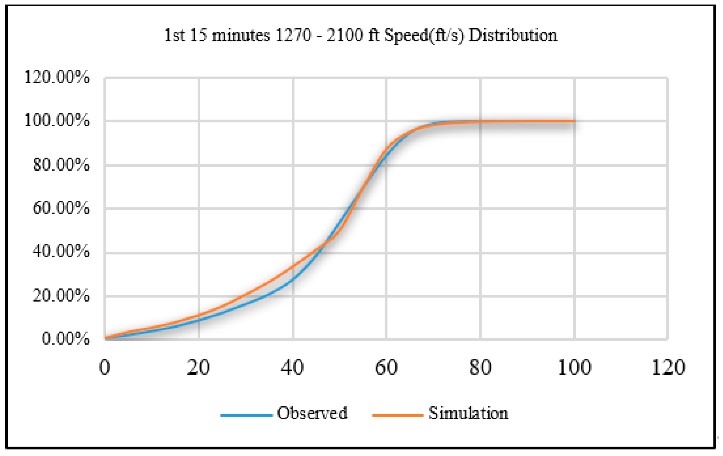
Figure 6 shows the comparison of the observed and simulated speed distributions. The simulation speed distributions match the empirical speed distributions very well, which means the selected speed distribution was successfully calibrated.
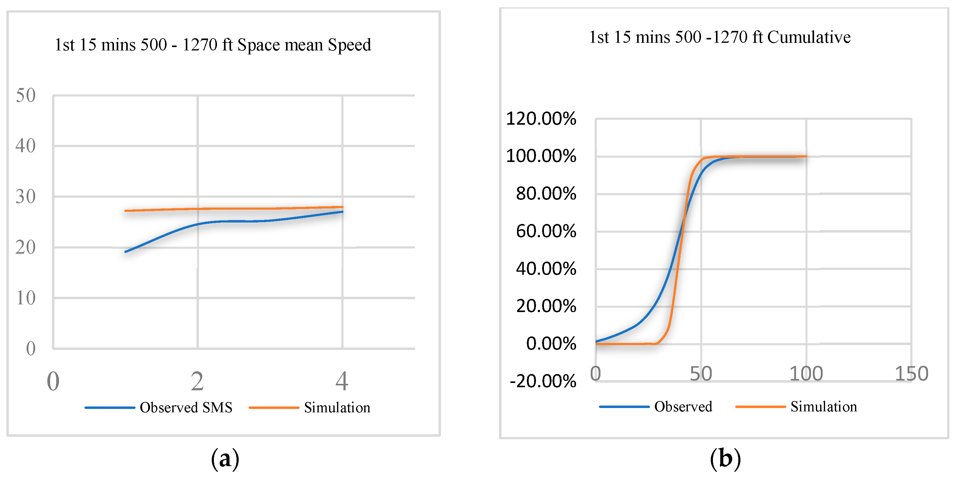
To calibrate for space mean speed and cumulative speed, data from the simulation output were collected from the second segment. The simulated speed range was between 25 and 50 mph. Using a similar speed distribution as the driver’s choice, both macro (space mean speed) and micro speeds (cumulative speed distribution) were calibrated. The simulation data collection point was selected at the midpoint of the second segment for lanes 1–4 from the left of the travel direction to examine traffic speed.
Figure 7 shows visually that both micro and macro speeds are calibrated successfully. The SMS for each lane and cumulative speed distribution for the second segment were compared with the calibration output as shown in
Figure 7 (for Macro level (a) and Micro level (b)). The
x axis shows the number of lanes and the y axis shows speed (ft/s
2) in
Figure 7.
We performed statistical tests to further verify whether the simulation output differed significantly from the observed data. A paired t-test at a 95% confidence interval was used. The null hypothesis was no difference between the means of the experimental and simulated speeds. The p-value of 0.103 was higher than 0.05, which means we fail to reject the null hypothesis. This implies that we had successfully calibrated the modeled speeds to the observed speeds.
4.3. Base Model Validation
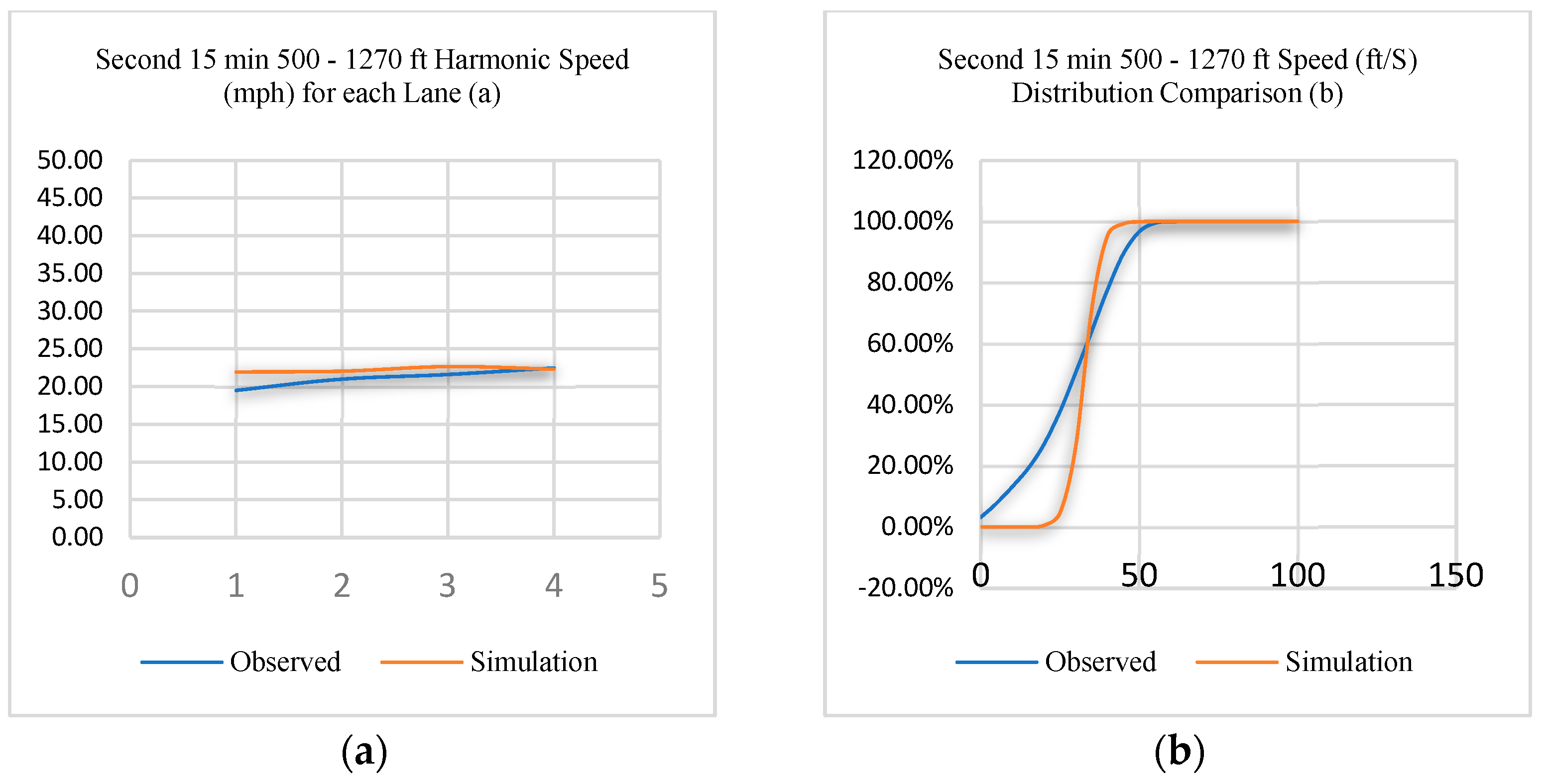
The next step in the modeling process was to validate the model against real-world data by comparing the calibration output from another period that was not used to calibrate the model. For validation purposes, the second 15 min were used. The SMS of lanes 1–4 from the left side and cumulative speed distribution of the middle section were compared to the observed data as shown in
Figure 8. Comparing the observed vs. simulation output visually for both micro and macro levels confirms that the simulations sufficiently replicate real-world observations.
A further paired t-test was performed at the 95% confidence interval with the null hypothesis that there was no difference between the means of the observed and simulated speed distributions. The p-value was 0.134, which is more than 0.05. This result means we fail to reject a null hypothesis that the means are statistically different from each other. This, together with the results from the calibration step, shows that the simulated model’s macroscopic and microscopic speeds are successfully calibrated and validated to the base observed data. The simulation model can therefore replicate real-life driving conditions for the case study area under oversaturated conditions. The next step was to develop the simulation model for the AV/CAV vehicle classes. The output from that step is then compared to the output from the base case to make inferences about the impacts of AVs/CAVs in mixed situations.
4.4. Wiedemann Simulation Parameters for the AV/CAV Vehicle Classes
The Coexist project [
42] proposed Wiedemann 99 CFM CC parameter values for different AV classes after numerous trials validated against real data. These parameters were adopted for this study shown in
Table 3. At the time of writing this research, this was the only study that had extensively used real-world data to evaluate and develop CC parameters that can be used to evaluate AV/CAVs will perform in traffic streams.
4.5. Simulation System Setup
A simulation system plays a significant role in replicating real-world data. Previous literature indicates that several simulation setup parameters such as the simulation resolution, the random seed, the number of runs, and the simulation speed could all influence the output of simulations (VDOT, 2020). The goal is to run a minimum number of simulations that provide optimal results given the time microsimulations take to run. To achieve this, the following equation was used to estimate the number of simulation runs and the other simulation system setup that were needed to get statistically significant results for this study [
43]
where,
R = Confidence Interval for the true mean t0.025,
N − 1= Student’s t-statistic for two-sided error of 2.5% (totals 5%) with N − 1 degrees of freedom (this is related to a 95% confidence level)
S = Standard Deviation about the mean for selected MOE
N = Number of required simulation runs
The parameters used in the simulation setup are listed in
Table 4.
5. Result and Discussion
To compare the impacts of AVs/CAVs on the transportation system for planning time horizons, we used output capacities as our method of evaluation. Capacities from the simulation are measured as the maximum passenger car/hr/ln. We develop several scenarios that include different mixes of AVs/CAVs, different penetrations of AVs/CAVs, and different forecast years. We first compare the capacities for single-class AVs/CAVs at different penetration levels. These scenarios assume that only one class of AV/CAV will exist at a time and gives a baseline capacity for each. It is probably an extreme case where either the technology never develops to the point where cars can drive themselves without significant human intervention, or the technology develops quickly enough where CAVs become predominant. Secondly, we introduce different mixes of AV/CAV technologies at different time periods to estimate the most plausible scenarios for AV/CAV impacts.
5.1. Base Model Capacities
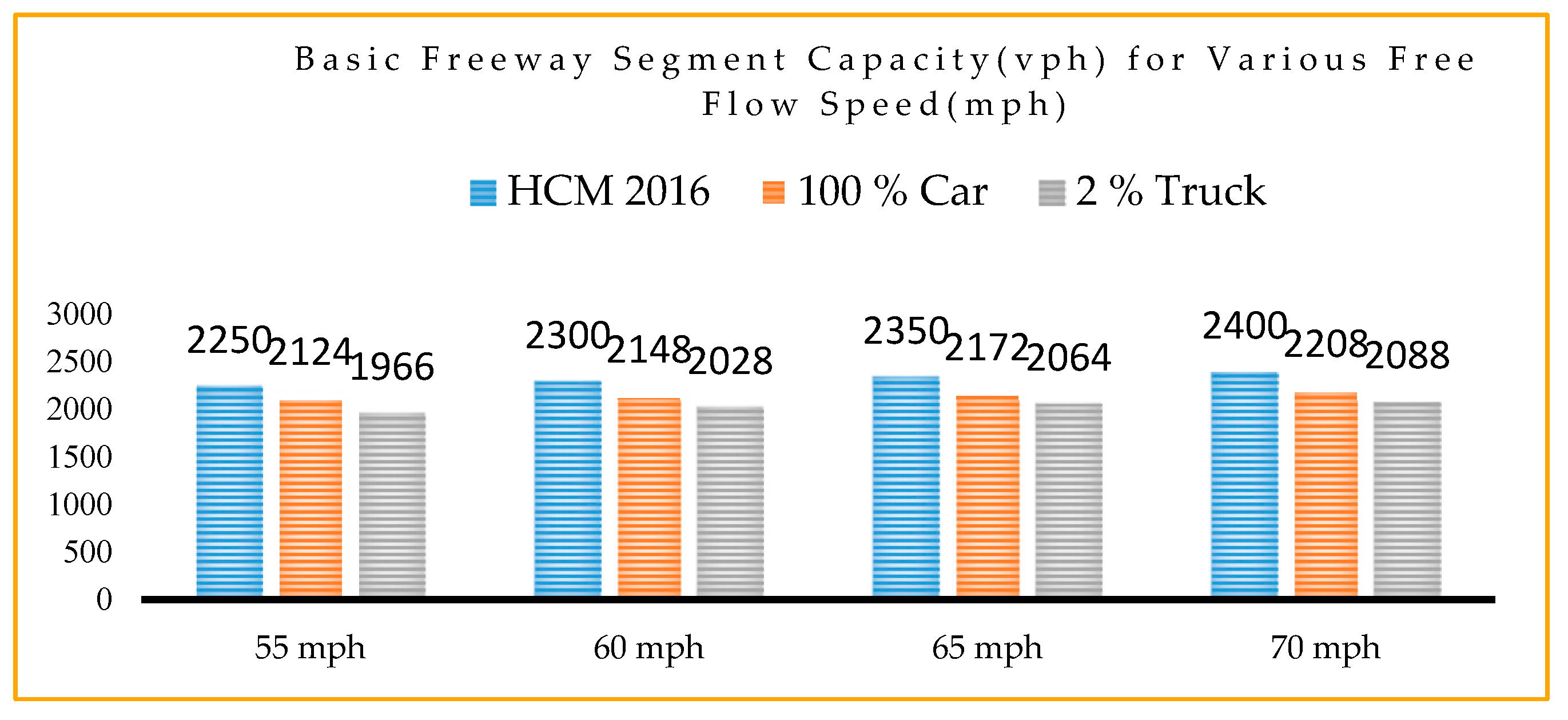
One of the major outputs of microsimulations is system capacity estimations.
Figure 9 shows the capacity output for the base case scenario. The base case includes two parts, a 98% passenger car scenario with a 2% heavy vehicle (truck) scenario, and a 100% car scenario. These two parts are compared to basic HCM published capacities for different free-flow speeds. The capacity from the simulation scenarios is on average about 11% lower than published HCM capacities [
44] for different free-flow speeds. This result emphasizes that real-world data should be used to estimate capacities that are used in simulation analysis. This is because although two roadways could be identical, driver behavior can significantly impact capacities.
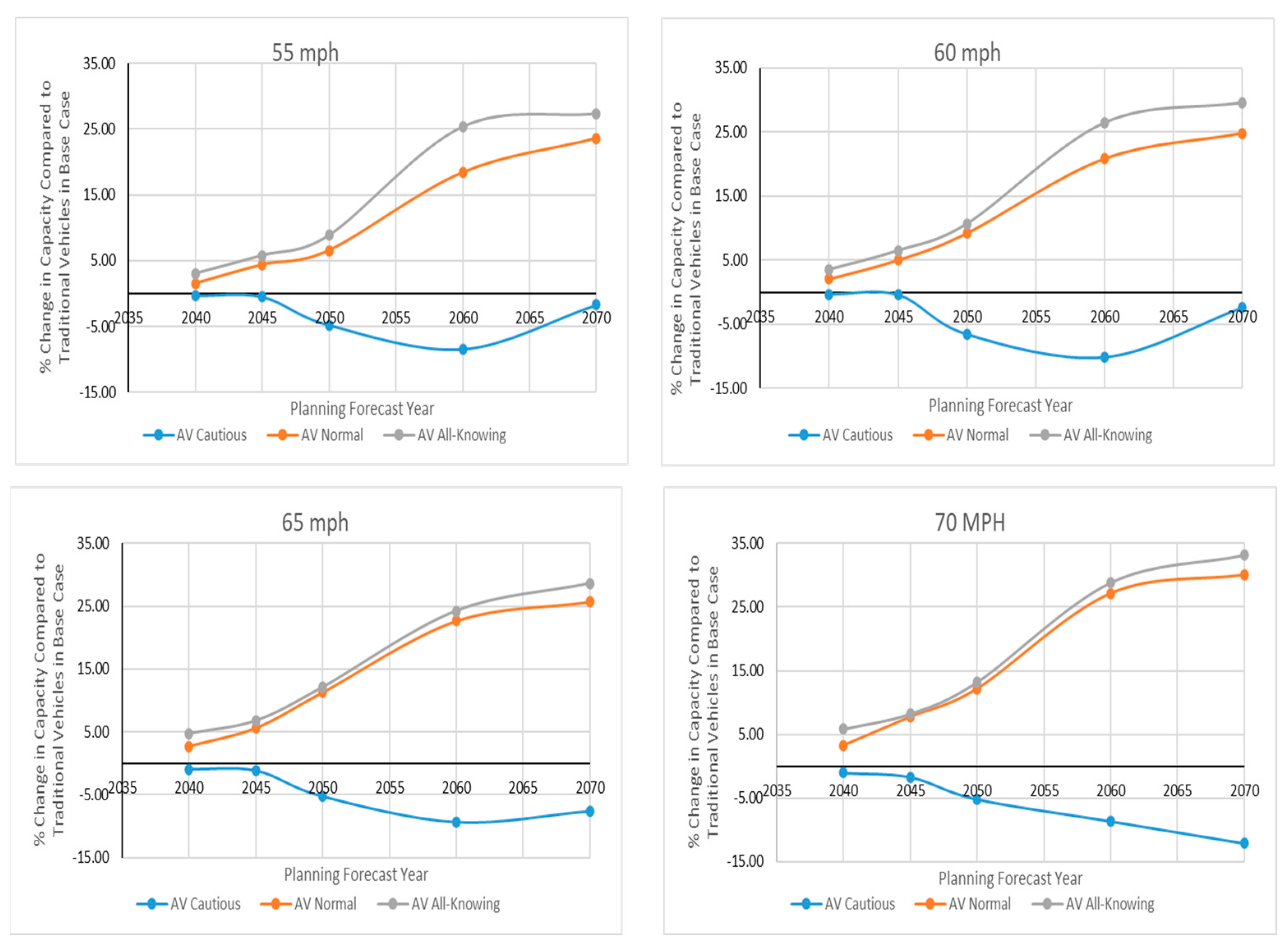
5.2. Capacities for Single-Class AVs/CAVs and Traditional Vehicles for Different Long-Range Planning Horizons
This section discusses the results when only one class of AV is used in each model for different speeds and different penetration levels. It assumes that we will not have more than one class of AV existing at any time.
Table 5 shows the assumptions used for the different mixes of AV/CAV penetration and traditional vehicles in this study. It shows for example that in 2040, 85% of all travel will be performed by traditional vehicles and 15% of travel will be by AVs/CAVs.
Figure 10 shows the comparisons of each AV class at different speeds and penetrations with the base model capacities that include only traditional vehicles. AV-cautious shows lower capacities for all penetration levels in comparison to traditional cars. The negative capacity impacts increase up to about 75% penetration where they begin to decrease but still stay lower than traditional cars. The lower capacity impacts are due to the algorithms assumed in these cars, which leave more headway between vehicles, as indicated by the Coexist study [
42]. Additionally, there is no Vehicle to Vehicle (V2V) or Vehicle to Infrastructure (V2I) communications in AV-cautious. These results suggest that for AVs to realize their true benefits, V2X should be incorporated into AV technologies, and driving behavior should be more responsive and aggressive. At present, Teslas and Audis can execute specific AV functions under certain road conditions. However, the time gaps (CC1 in the Wiedemann model) these vehicles maintain for safety purposes are longer, allowing traditional vehicles to cut in front of them in a travel stream. This effect is further compounded in oversaturated conditions, where their bumper-to-bumper headways (CC0) are longer than current traditional vehicles in the dataset. Although AV-cautious technologies defined in this study might be the first to be implemented, a combination of regulations, lack of trust, and potential legal issues for manufacturers may play a part. These findings underscore the need to consider AVs’ potential capacity reductions and their impact on transportation planning efforts, and the importance of incorporating V2X into AV technologies.
The AV normal and AV all-knowing (CAV) classes have capacity gains for all speeds and penetration levels as shown in
Figure 10 in comparison to traditional vehicles. AV all-knowing shows higher capacity gains than AV-normal as expected. Vehicle sensors, connectivity, and vehicle response are quicker than in traditional vehicles, resulting in lower CC0 and CC1. These vehicles, as expected, will leave lower time and space gaps between a lead and the following vehicle thereby increasing capacities without changing the transportation supply. These vehicles will become more available as technology becomes mature and confidence in them grows both among the public and decision-makers. The capacity impacts are linear up to about 40% penetration levels where they increase exponentially and taper off at 80% penetration levels.
5.3. Capacities for Mixed AV/CAV/Traditional Vehicle Classes for Different Long-Range Planning Horizons
To evaluate the potential impacts of AV/CAVs for different penetrations and different mixes, we develop demonstrative scenarios that allow for a more focused analysis over various planning horizons. The scenarios were developed to test different levels of AV penetration for the different AV classes for each of the forecast years, which range from mid-range (20 years) to long-range (25–35 years) and buildout (beyond 35 years). These scenarios test the impacts that technology in AV will have on highways over different planning horizons. The number of possible scenarios is infinite; however, two demonstrative scenarios are discussed. These are based on AV/CAV projection literature ([
12,
45,
46]), testing by the researchers, vehicle ownership turnover, and intuitive assumptions of technology advancements for AVs.
Scenario 1: Conservative technology scenario: assumes relatively slow technology development and that AV-cautious will be the dominant technology, representing a significant proportion of AVs.
Scenario 2: Optimistic technology scenario: assumes quicker technology development and that AV-all-knowing will be adopted and deployed faster in the vehicle populations.
Next, we will discuss the assumptions for each mixed scenario and their capacity impacts compared to the base case of traditional vehicles for the different forecast years. The assumptions represent the amount of travel by each of the different vehicle types and not the total vehicle class. These results will be discussed in more detail below.
Table 6 shows the AV/CAV mixed scenario assumptions and capacity impacts for the forecast year 2040 which can be considered mid-range for planning purposes. For the conservative technology scenario, the impact of having only AV-cautious means that basic freeway capacities will potentially decline. The capacity impacts range from −0.31% to about −1.92%. For the optimistic technology scenario, the capacities also decline but with comparatively lower impacts compared to the conservative technology scenario. The implication for planners is that they must develop traffic management strategies to manage capacity reduction rather than increasing capacities.
Table 7 shows the AV/CAV mixed scenario assumptions and capacity impacts for the forecast year 2045 for different AV-cautious, AV-normal, and AV-all-knowing penetrations for the two scenarios. The basic assumption is that we will have a 25% AV/CAV fleet and 75% traditional vehicles in traffic by 2045 [
12]. The conservative technology scenario shows that capacities will increase marginally between 1.5% and 3% compared to traditional vehicles. The optimistic technology scenario also shows that capacity gains will range between 2% and 3.93%. The results show that capacity gains due to AVs/CAVs will be marginal within the next 25 years which is within long-range horizon plans for most planning agencies in the U.S.
Table 8 shows the capacity impacts and AV/CAV mixed scenario assumptions for the forecast year 2050, assuming a 40% penetration level of AV/CAVs. For the conservative technology scenario, capacity gains are modest, ranging from 1.93% to 3.5%. However, for the optimistic technology scenario, capacity gains start to become significant, with an increase of 5.98% for the 70 mph roadway. This is over two percentage points higher than the conservative technology scenario. The current 30-year long-range planning horizon for transportation planners falls within the forecast year 2050. Our findings suggest that although capacities may decline in the short term, they will begin to improve in the long term. As such, planners may not necessarily need to invest in increasing highway capacities in the short term to account for the decline that is shown in
Table 6.
To address short-term negative impacts on capacity, transportation planners could consider implementing measures to reduce demand or improve travel efficiency, such as promoting public transit use, implementing congestion pricing, or optimizing signal timing. Additionally, planners can consider incorporating more AVs/CAVs in their planning models to better assess and plan for their impacts on capacity. By doing so, planners can make informed decisions about the best use of their resources and investments in the short and long term. It is important to consider the potential negative impacts of lower AV technologies and penetration levels, as they may reduce capacity and lead to increased congestion in the short term.
Table 9 presents the capacity impacts and AV/CAV mixed scenario assumptions for the forecast year 2055, with an assumed AV/CAV penetration level of 50% of total travel. The conservative technology scenario shows modest capacity gains of between 2.54% and 3.93%, while the optimistic technology scenario shows significant capacity gains ranging from 4.29% to 7.76%. On average, the capacity impact for the optimistic technology scenario is about three percentage points higher than that of the conservative technology scenario. These findings are particularly relevant for transportation planning efforts, as the planning horizon for 2055 falls within the long-range planning horizon for many agencies.
Table 10 summarizes the AV/CAV mixed scenario assumptions and capacity impacts for the forecast year 2060, assuming that AV/CAVs will make up about 60% of total travel. For the conservative technology scenario, the capacity gains start to become significant, ranging from 5.6% to 7.47%. The capacity gains for the optimistic technology scenario become even more significant, ranging from 9.87% to 12.07%. On average, the capacity impact for the optimistic technology scenario is about four percentage points higher than that of the conservative technology scenario. These results suggest that transportation planners and decision-makers will start to see the meaningful impacts of AVs/CAVs around the forecast year 2060, which is beyond most long-range planning horizons but could be used for full buildout planning scenarios that consider data beyond the long-range planning horizons. The findings highlight the importance of considering AV/CAV technology and penetration levels in transportation planning efforts over various planning horizons.
Table 11 shows the AV/CAV mixed scenario assumptions and capacity impacts for the forecast year 2070 which assumes that AV/CAV will make up about 90% of total travel. For the conservative technology scenario, the assumption is that the bulk of the AV vehicles will be AV-cautious and AV-normal vehicles. This scenario sees capacity gains ranging from 10.13% to 17.33% compared to traditional vehicles. The optimistic technology scenario assumes that half of the AV vehicles will be AV-all-knowing, and the other half will be AV-cautious and AV-normal vehicles. The capacity gains for this scenario range from 15.91% to 21.29%, which will make a big impact on capacity decisions on highway transportation systems.
Table 12 shows the AV/CAV mixed scenario assumptions and capacity impacts for the forecast year 2080 which assume that AV/CAV will make up about 100% of total travel. For the conservative technology scenario, the assumption is that AV-all-knowing will make up 60% of the travel whereas AV-cautious and AV-normal will make up 40% of total travel. This scenario sees capacity gains ranging from 16.48% to 22.99% compared to traditional vehicles. The optimistic technology scenario assumes that 80% of the AV vehicles will be AV-all-knowing and the rest will be AV-normal vehicles with no AV-cautious vehicles. The capacity gains for this scenario range from 22.99% to 29.31%.
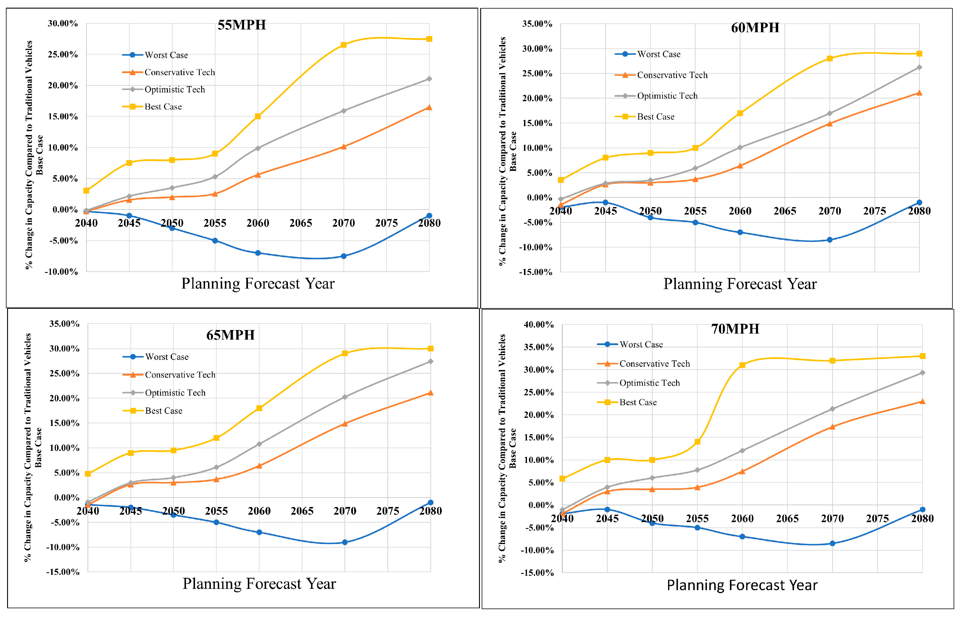
5.4. Transportation Long-Range Planning Horizon Capacity Comparisons Summary
The overall capacity impacts of AV/CAV technology scenarios and penetrations are summarized in
Figure 10 for medium-range, long-range, and buildout planning horizon years. The worst-case scenario assumes only AV-cautious technology will be adopted, whereas the best-case scenario considers the implementation of only AV-knowing. The conservative and optimistic technology scenarios consider different combinations of AV-cautious, AV-normal, and AV-all-knowing technologies, along with various levels of traditional vehicles. In the medium-range planning horizon, capacities may decrease as seen in the worst-case scenario and both the conservative and optimistic technology scenarios. However, in the long-range planning horizon, capacities will start to increase modestly, as indicated by the conservative and cptimistic technology scenarios from 2045 to 2055. Beyond 2055, the capacity impacts of AV/CAV will become more significant and positive in the buildout scenarios. Thus, the technology in the vehicles will have a crucial impact and transportation planners must consider these impacts in their plans.
Our findings reveal that the technology of AVs/CAVs plays a crucial role in determining their impact on capacities. In the medium-range planning horizon, capacities may decrease as seen in the worst-case scenario and both the conservative and optimistic technology scenarios. This suggests that planners must take into account the negative impacts of low AV/CAV penetration, particularly in urban areas. However, in the long-range planning horizon, capacities will start to increase modestly, as indicated by the conservative and optimistic technology scenarios from 2045 to 2055. This indicates that AVs/CAVs have the potential to alleviate capacity issues in the long term but not in the short term.
Figure 11 summarizes the results of this study and shows the planning horizon capacity impacts of AV/CAVs.
6. Conclusions and Discussion
This research aimed to assess the impact of AVs/CAVs on transportation system capacities via simulation-based analysis, with the objective of determining the effect of different AV/CAV technologies on capacities over various planning horizons. A microsimulation model was developed using real-world data and calibrated to model only traditional vehicles, which was then expanded to incorporate AV/CAV technologies using data from the Coexist project. Using current projections for AV/CAV penetrations, impacts were estimated for three planning horizons. The results of this study provide valuable insights for transportation planners and decision-makers in making medium and long-term transportation decisions regarding the impact of AVs/CAVs.
One important finding of this study is that low AV penetration with lower AV technologies, specifically AV-cautious technology at all levels and in mixed scenarios with traditional vehicles, will result in reduced capacities compared to traditional vehicles. According to the AV/CAV forecast literature, this is what will happen in the medium-term transportation planning horizons. Higher penetrations of AV all-knowing technologies will result in increased capacities at all penetration levels. These findings highlight the need for transportation planners and decision-makers to consider the potential impacts of AV/CAV technologies on transportation system capacities over various planning horizons. This study provides valuable information on the potential impacts of AVs/CAVs on capacities over various planning horizons, as well as the need for creative solutions to declining capacities at low penetrations of AVs, particularly in urban areas. Short-term measures such as optimizing the use of existing infrastructure, improving transit options, and promoting active transportation could help address capacity issues in the mid-term. As AV/CAV penetrations increase and capacity impacts become positive in the long term, planners could consider investing in new infrastructure, such as dedicated AV/CAV lanes and interchanges, to support the growth of AV/CAV technologies.
However, the study is subject to several limitations. One limitation is that the forecast of AV penetrations is constantly changing, which could affect the accuracy of the study’s projections. Another limitation is that the simulation model does not account for the potential impact of AVs on travel demand and mode share, which could affect the results. Additionally, the oversaturated traffic data used in the study may not be representative of all traffic conditions, and the assumptions made about the behavior of AVs/CAVs may not reflect reality. Future studies could explore these limitations in more detail and consider other factors, such as the impact of AVs/CAVs on travel demand, mode share, and driver behavior, as well as different traffic conditions, infrastructure configurations, and vehicle types.
The findings of this study highlight the need for transportation planners and decision makers to consider the stochastic effects of AV/CAV penetration on transportation planning efforts. Overall, this study provides important information for transportation planners and decision makers to consider as they develop medium and long-term transportation plans and make informed decisions about the impact of AVs/CAVs.


