1. Introduction
A traffic monitoring system is an effective method of easing traffic congestion. It is an integral part of the intelligent traffic system (ITS), which is used to collect traffic data such as the number of vehicles, vehicle type and vehicle speed. Based on the collected data, it performs traffic analysis to make better use of the road system, predict future transportation needs and improve traffic safety as it is one of the exhibition traffic infrastructures in which traffic authorities invest large sums of money to collect and analyse traffic data to make better use of the road system. Urban roads and highways currently have multiple surveillance cameras initially installed for various security reasons. Traffic videos from these cameras can be used to estimate traffic conditions and automatically identify traffic jams, accidents and violations, helping traffic managers deal with important aspects of traffic. Increasing the accuracy of vehicle classification has a very positive impact on traffic monitoring systems [
1].
Intelligent transportation systems (ITS) are systems that use advanced technologies, such as sensors, cameras and communication systems, to improve the safety, efficiency and sustainability of transportation networks [
2]. Fine-grained vehicle classification is a key component of ITS as it allows transportation systems to identify and classify individual vehicles accurately. This information can be used to optimise traffic flow, improve safety and reduce emissions by enabling targeted measures such as dynamic routing and intelligent speed adaptation.
Computer vision (CV) and deep learning (DL) are becoming popular research areas among students and researchers. The latest advancement in deep learning has significantly improved computer vision performance in various application areas such as intelligent transportation, medical image analysis, facial detection, etc. [
3]. Computer vision enables computers to observe and understand the world in the same way humans do. It involves developing algorithms and systems that can analyse, interpret and understand visual data from the world around us, such as images and videos. The human eye is limited to seeing only RGB (red, green and blue) and grayscale images, whereas computer vision can gather much more information than the human eye, such as the segmentation of objects, the height of objects’ edges, pixels, infrared (IR) information and several other minute details.
Vehicle classification is an application found on all vehicle passageways, such as motorways, main highways, car parks and access roads leading to rest areas. The main objective is to detect the different types of vehicles to optimise infrastructures and increase the return on toll gates by traffic flows. As vehicle classification is a fundamental part of intelligent transportation systems and is universally used in traffic surveillance, traffic flow control and security coercion, the accuracy of vehicle classification data plays a crucial role in proper future highway and road design by increasing road traffic safety and annihilating traffic jams [
4]. Any loss of accuracy in vehicle classification, even of the order of 1%, swiftly causes a notable economic deficit; hence, vehicle classification is very arduous.
Improvements in vehicle classification accuracy have a significant impact on traffic surveillance and traffic flow monitoring. Traffic video surveillance can help in traffic control and gathering traffic statistics that can be used in intelligent transportation systems [
5]. Due to the good accuracy of vehicle classification, the interactions between travellers and infrastructures become ideal.
Some road vehicles are classified into a broad range of classes according to their distinctive behaviours and safety measures due to the increase in accuracy of this classification of road safety, which is extended by notifying vehicles of dangerous situations on the road. This problem affects many aspects of modern society, including economic development and traffic accidents [
6]. Over 70% of the weight of goods shipped in the U.S. are trucked and substantial pavement damage is becoming more problematic. Any inaccuracy in vehicle classification has a negative impact on traffic surveillance because it weakens interactions between travellers and infrastructures by reducing road traffic safety and increasing traffic jams. Vehicle classification accuracy loss has a negative impact on road design and will jeopardise future highways.
In this study, four DCNN models were analysed on three different datasets to compare their performance.
The following points summarise the contributions of this research.
A detailed review investigates the most promising work in the machine/deep learning domains for the fine-grained classification of vehicles.
A new dataset PAKCars has been created which contains 44 models of 9 makes of Pakistani cars.
A comprehensive analysis of DCNN models on fine-grained vehicle classification with three different datasets is presented.
This study highlights the trade-off between the accuracy of DCNN models, which assists researchers/students in selecting hardware for implementations.
In this study, the proposed algorithm for data augmentation produces much fewer images, which helps to reduce training time.
The research is further organised as follows.
Section 1 discusses the literature related to this study.
Section 2 describes the materials and methods of this research, which incorporates DCNN models, datasets, data augmentation, training and testing processes, system setup, and comparisons with related work. Further,
Section 3 presents and discusses the results. The conclusion of the study is found in
Section 4.
2. Literature Review
Recent advancements in deep learning have drastically enhanced the performance of machine vision in several application areas. In image processing, the challenges of object recognition and categorisation are crucial. Each item has its own distinct qualities. Object detection provides information about the object’s position, whereas object categorisation provides information about the object’s class. Object classification is a technique for identifying specific real-world items that are based on the machine-learning field of image processing.
In [
7] this research, the authors proposed a fully automated system recognising models and colours. The proposed system was implemented using ImageNet. This type of visual classification and identification is always complicated in terms of precision and efficiency [
8,
9,
10,
11]. The system involves three steps, which include collecting datasets, pre-processing images and deep learning. The publicly available dataset, Stanford Cars, that was used to test the proposed system consists of 196 classes and 16,185 images [
12] and uses CompCars to achieve high performance.
In addition, Sighthound’s approach, which uses deep neural networks trained on a large dataset for training and can accurately label vehicles in real-time, was proposed by the author of [
7] for vehicle make and model recognition.
In another study, the author [
13] proposed a novel method for combining local features with different viewpoint angles in a similar layout to improve the standard of MI-SVM formulation; this method is known as the iterative multiple-learning method and is used for vehicle classification and view-point labels with high precision. In this study, the authors investigated the outcomes of the proposed model using two distinct datasets, INRIA and Stanford Cars, and compared their results in terms of classification accuracy using various attribute selection methods and varying degrees of viewpoint supervision. Combining attribute features with low-level Fisher vector features [
14] and applying a simple mixing method to the normalised scores of each test image yielded the desired outcome.
In these studies [
15,
16], researchers also offered an additional technique for LIDAR-based vehicle detection. LiDAR, or laser detection and ranging, is a technology that was evolved from radar. On this platform, a vast number of point clouds are provided by LiDAR that are used to detect objects. Additionally, trained SVM, CNN and DCNN models are utilised for the classification of cars and non-vehicles. In a separate study, the authors demonstrated vehicle identification at larger distances using the 3D LIDAR technique. For image object segmentation, the technique RGLOS (Ring Gradient Based Local Optimal Segmentation) was utilised. Three types of features were extracted for feature extraction in one study [
17] regarding position-related shape, object height along the length and reflective intensity histograms.
3. Materials and Methods
This study sought to develop vehicle fine-grained classification using diverse DCNN architectures by utilising three different datasets. The methodological procedure can be broken into two steps: a CNN-based training process and testing of the trained model process.
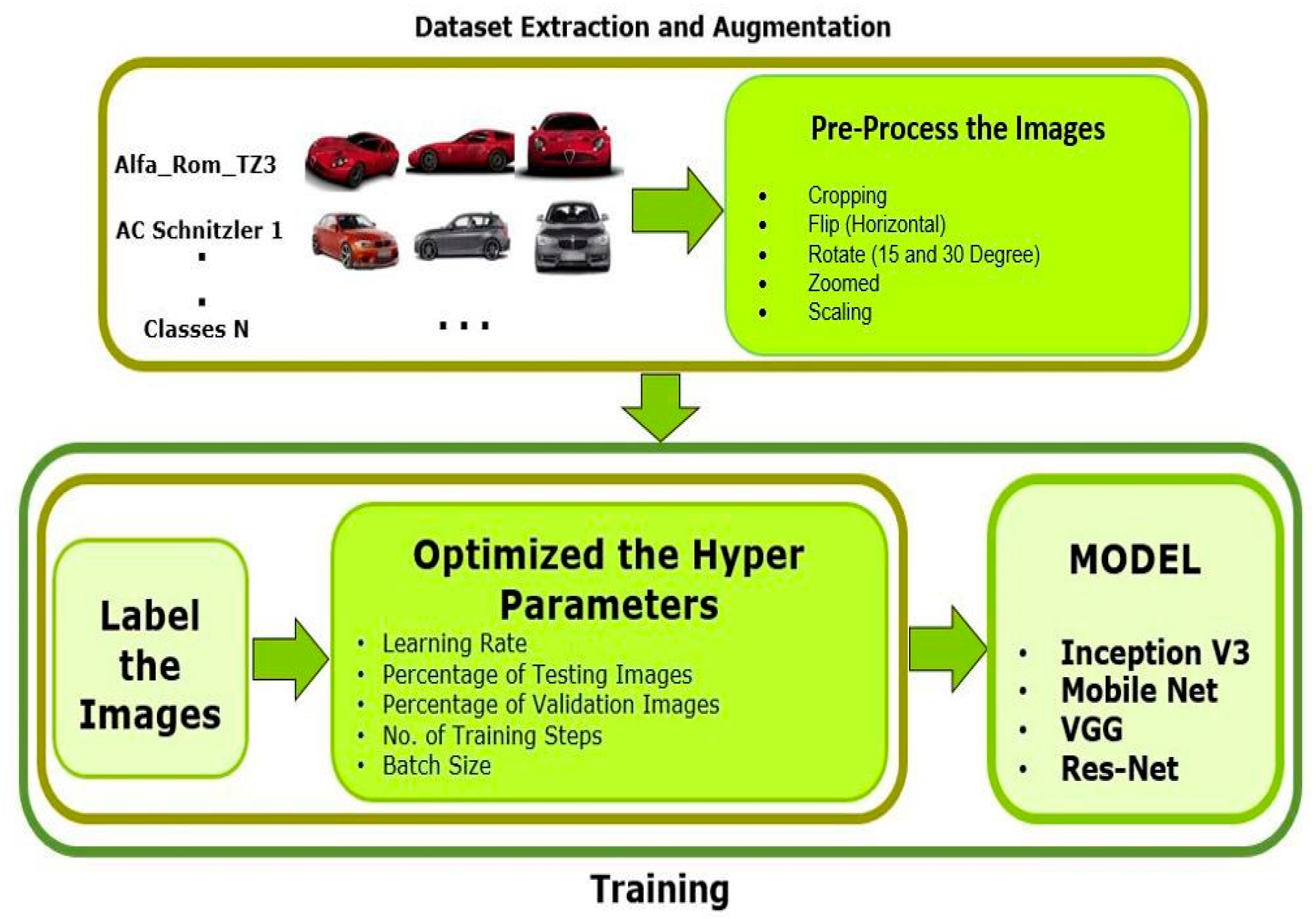
Figure 1 depicts the methodology’s workflow and
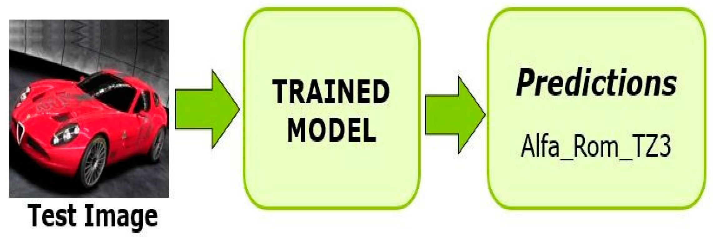
Figure 2 depicts the testing procedure. As stated in
Table 1, the datasets utilised by the system were BMW-10, Stanford Cars and PAKCars. In this study, a recently created dataset was utilised that enabled researchers to efficiently classify commonly used cars in Pakistan. The authors modified the accessible datasets (BMW-10, Stanford Cars) by snipping raw images from the specified bounding box and classifying images with their relevant car’s make and model directories using the provided labels for the testing and training sets. In addition, a state-of-the-art dataset, PakCars, was created specifically for use in this research, which is also arranged like the other two datasets, in which each manufacturing company and model are separated into separate folders. After the preparation of the dataset, some preprocessing of images was required before they were fed to the CNN models for training. For pre-processing, first, all images were resized at the same scale and then image augmentation techniques were applied to enhance the dataset such as flipping, zooming, rotating and rescaling. The datasets were then ready for CNN model training. The trained models with preprocessed data achieved distinct results, which were then validated.
The datasets were pre-processed before training the CNN models. Flipping, rotating, zooming and re-scaling images were image augmentation techniques conducted during the pre-processing stage. The datasets were trained on numerous different DCNN models (MobileNet-V2, Inception-V3, VGG-19 and Residual-Net-50). The models trained using pre-processed data obtained different results, which were then validated.
3.1. Architectures Used to Implement CNN
The structure of CNNs has been continuously improving since 1989. These improvements can be classified as regularisation, parameter optimisation and structural reformulation [
18]. Some common CNN models are LeNet, Alexnet, VGG, GoogleNet, Inception-V2, Inception-V3, Inception- V4, ResNet and MobileNet.
The following CNN models were used in this research.
Mobilenet-V2
Inception-V3
VGG-19
Resnet-50
3.1.1. Mobilenet-V2
The mobilenet architecture was proposed by Google and is based on a streamlined architecture. Due to its lower computational cost, it is used to build lightweight networks. Mobilenet executes a single convolution on each colour channel. It does not combine and flatten all three RGB channels; this has the effect of filtering the input. It is beneficial for both mobile and embedded systems. This architecture is also suitable where there is a lack of computational power. It replaces normal convolution with depth and point-wise convolution, which is called depth-wise separable convolution [
19]. In standard convolution, a convolution is parameterised by kernel
K size
Dk ×
Dk ×
M ×
N; here,
Dk is the kernel size spatial dimension (square), M is the number of input channels and N is the number of output channels.
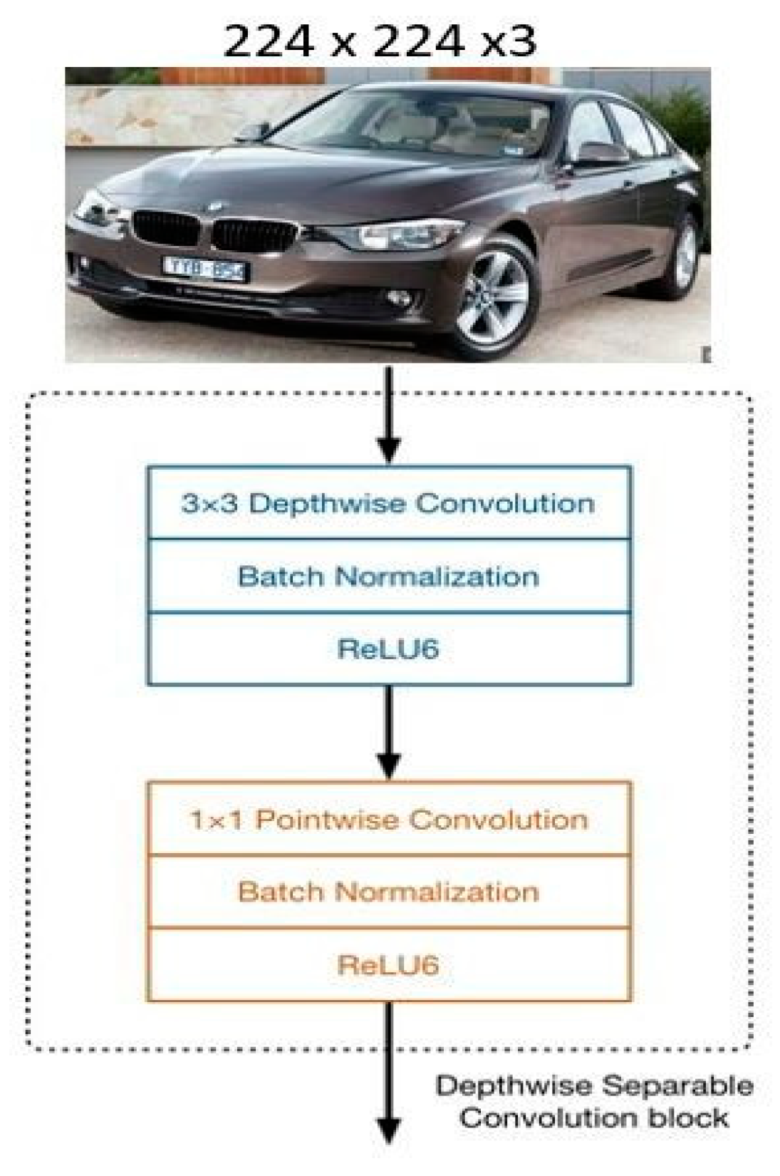
The foundation of the mobilenet model is depth-wise separable convolutions, a type of factorised convolution that factors a standard convolution into a depth-wise and point wise convolution. Point-wise convolution, also known as 1 × 1 convolution, is a type of convolution where the kernel size is 1 × 1. It is used to adjust the number of channels in an input feature map, while preserving the spatial resolution of the feature map. Depth-wise convolution, on the other hand, is a type of convolution where the kernel is applied to each channel of the input feature map separately. It is used to extract features from each channel independently. Combining the results of point-wise and depth-wise convolutions can be useful for extracting both channel-wise and spatial features from an input feature map. Standard convolutions combine inputs into a new set of outputs in one step while also filtering the inputs. This is divided into two layers by the depth-wise separable convolution—a layer for combining and a layer for filtering. The computation and model size are significantly decreased as a result of this factorisation. An example of the factorisation of the depth-wise separable convolution block is shown in
Figure 3.
3.1.2. Inception-V3
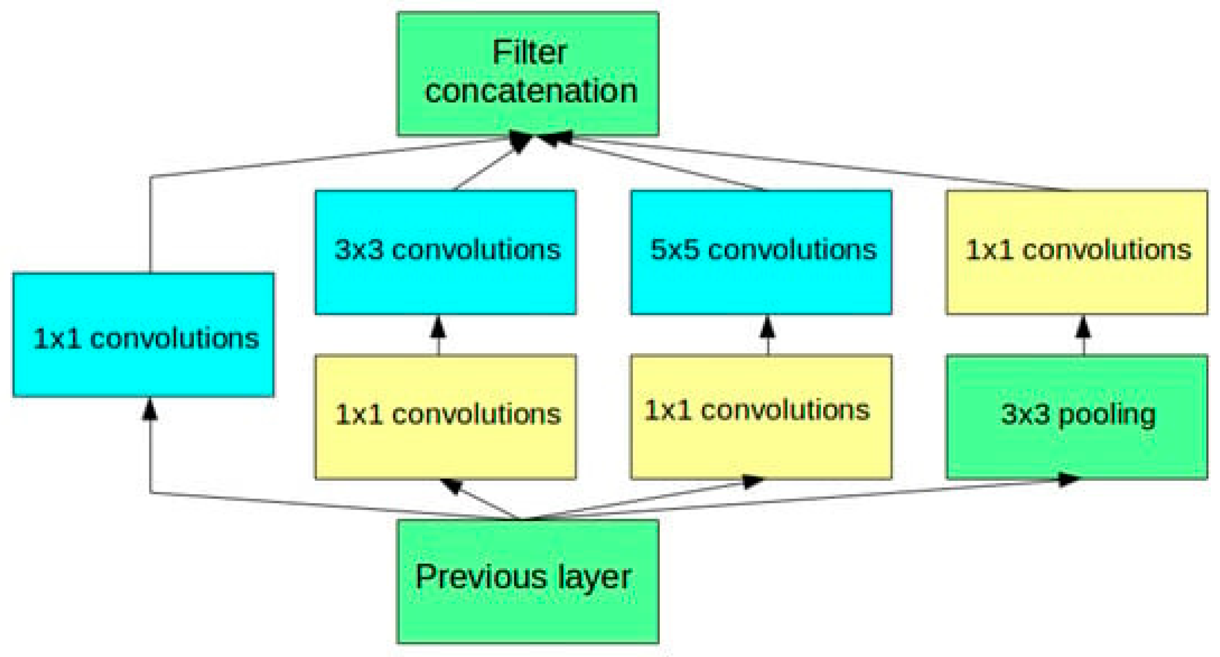
A popular image classification or recognition model with high accuracy rates is inception-V3, which was used in this study. The inception-v3 model is composed of symmetric and asymmetric blocks. It has various layers, including convolution, max pool, fully connected, concat, average pool, dropout and softmax. These layers have been used to carry out intricate computations on datasets. The direction of the layers clearly demonstrates that the information flow is feed-forward layer by layer; thus, it will limit the number of convolutions to a maximum of 3 × 3 to avoid complexity. The complete architecture of inception-v3 is shown in
Figure 4.
3.1.3. VGG-19
VGG-19 had greater depth compared to AlexNet and was very uncomplicated. The model supports 19 layers, indicating the number of convolutional layers present in the model. The model has three layers more than VGG-16. Model VGG-19 specified the structure, colour and shape of the image very well as it has pre-trained layers with advanced CNNs. The sequence of the 3 × 3 convolution filter was used by the VGG-19 network. Additionally, there were two prime inadequacies of this model: (1) As VGG19 consists of 19 layers with the same size filters due to the depth lots of parameters involved in computation, the training process is slowed due to a large number of calculations. (2) Some features are overlooked due to using the same size filter throughout the network design. The backpropagation algorithm updates the weights of a neural network, slightly modifying each weight so that the model’s loss is reduced. In order to move towards reducing loss, it updates each weight. It simply records the weight’s slope, which can be determined using the chain rule. The value, however, continues to rise with each local gradient as the gradient continues to flow back to the beginning layers. The alterations to the earliest layers are consequently drastically reduced as the gradient gets smaller. This causes some features to be overlooked and increases the training time.
3.1.4. ResNet-50
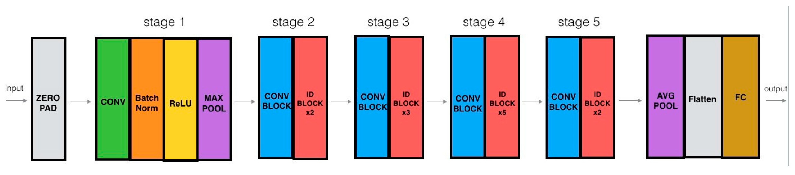
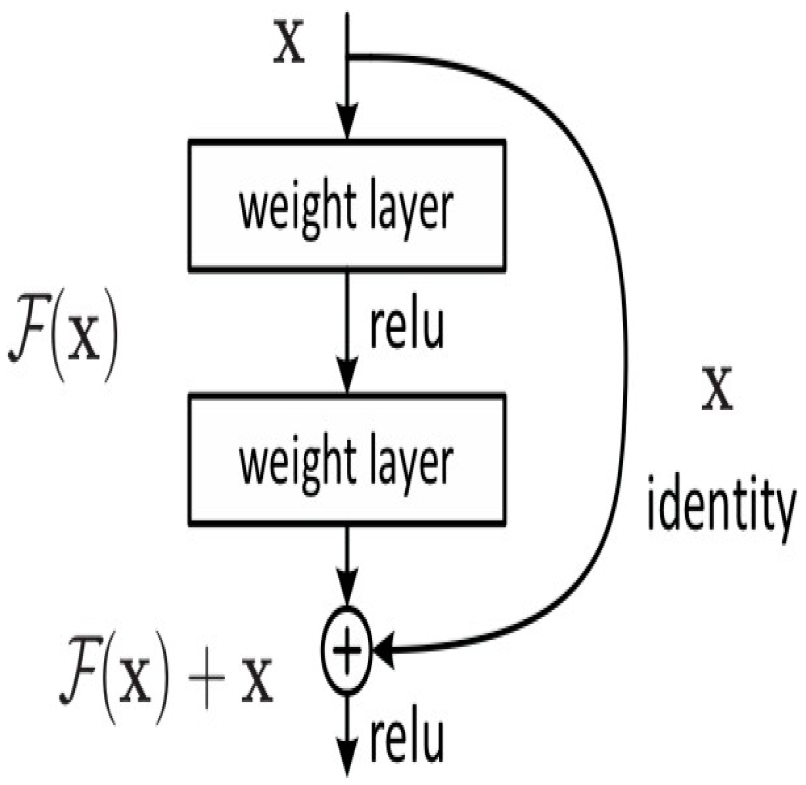
ResNet-50 is a 50-layer deep convolutional neural network that was introduced by Microsoft in 2015. A variant of the model that can work with 50 layers of the neural network is resNet-50. resNet-50 is used as a starting point for learning transfer and is considered a smaller version of resNet-152. In many computer vision tasks, it plays a vital role. This model is able to classify images into thousands of categories of objects such as Desks, pens and many animals. ResNet-50 models consist of 50 layers; they have 1 average pool layer and 1 max-pool layer with 3.8 × 10⁹ floating point operations. They also enhance the performance of neural networks with more layers and fewer errors. ResNet-50 is also used to connect the input of the nth layer to some (n + x)th layer directly by using shortcuts. The image input size in this model was 224-by-224. Using this model was easy compared to other deep convolutional neural networks. Degrading accuracy problems are also resolved by resNet-50. Five stages are involved in this model and each stage has its own identity block and convolution, while each identity block and convolution further have convolution layers of 3 × 3. Over 23 million trainable parameters are contained in ResNet-50. The layer-by-layer architecture of the resnet model is shown in
Figure 5.
Figure 6 shows a logical scheme of the base building block of ResNet-50.
3.2. Datasets
In machine learning, the selection of the data set is of critical importance. Once a model has been developed, the network must be trained using a dataset. The dataset is a collection of samples such as images or text data and an essential part of any machine learning system as all predictions are based on the given dataset. Datasets are usually divided into two parts: training and testing. The training part is used to train the machine and the testing part is used to validate or test the trained machine.
To perform the classification of cars based on their features, a dataset of cars is needed that must contain the makes and models of the cars. This study utilised the following datasets:
Stanford Cars
BMW-10
PAKCars
3.2.1. Stanford Cars
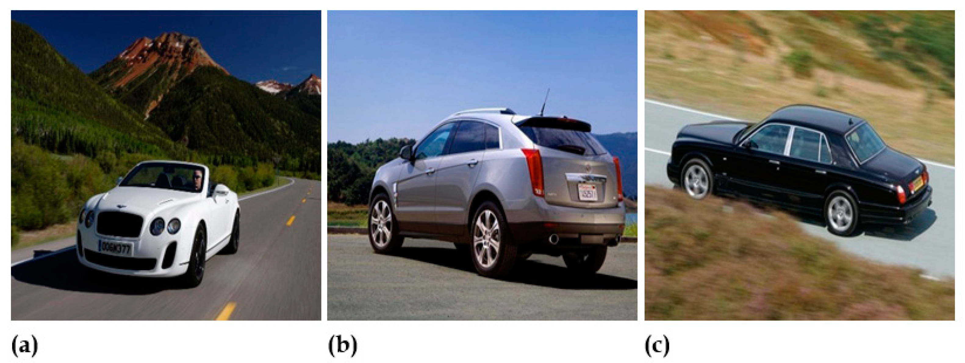
The Stanford Cars dataset contains 196 classes with makes and models. The total number of images contained in the dataset is 16,185. The dataset was divided into two parts: testing and training. The numbers of images used for training and testing were 8144 and 8041, respectively. Thus, the dataset was almost divided equally (50/50). Typically, a car dataset is categorised based on make, model and year; this means that multiple classes will have the same make and model but belong to a different manufacturing year [
11]. Examples of randomly selected images from the Stanford Cars dataset are shown in
Figure 7.
3.2.2. BMW-10
The BMW-10 dataset is an ultra-fine-grained classification dataset. The dataset contains 10 classes. The dataset contains 511 images with an average of 50 images per class. Examples of randomly selected images from the BMW-10 dataset are shown in
Figure 8.
3.2.3. PAKCars
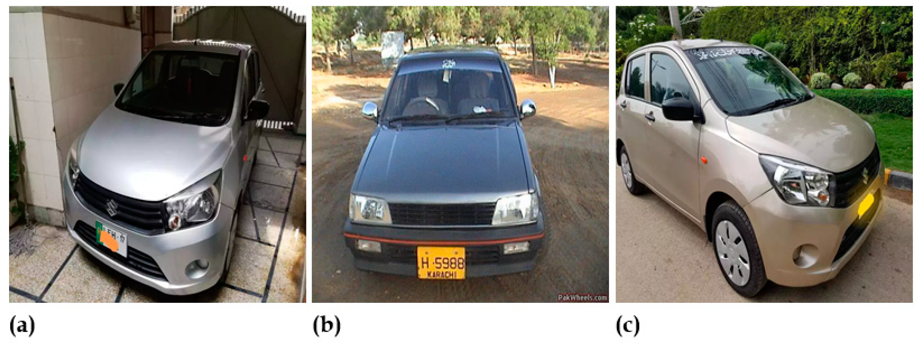
Th PAKCars dataset is generally for cars commonly used on Pakistan’s roads; it is utilised for fine-grained vehicle classification and can also be utilised in other countries where these cars are used. There is a limited number of data points. The images are taken from different angles and perspectives. The detection and classification of vehicles in Pakistan are made possible by this system. The dataset contains the models of cars made from the 1980s to 2018. It contains 40 classes and each class has 50 images. It contains a total of 2000 images. The dataset is equally divided into two parts: testing and training. Examples of randomly selected images from the PAKCars dataset are shown in
Figure 9.
3.3. Dataset Extraction
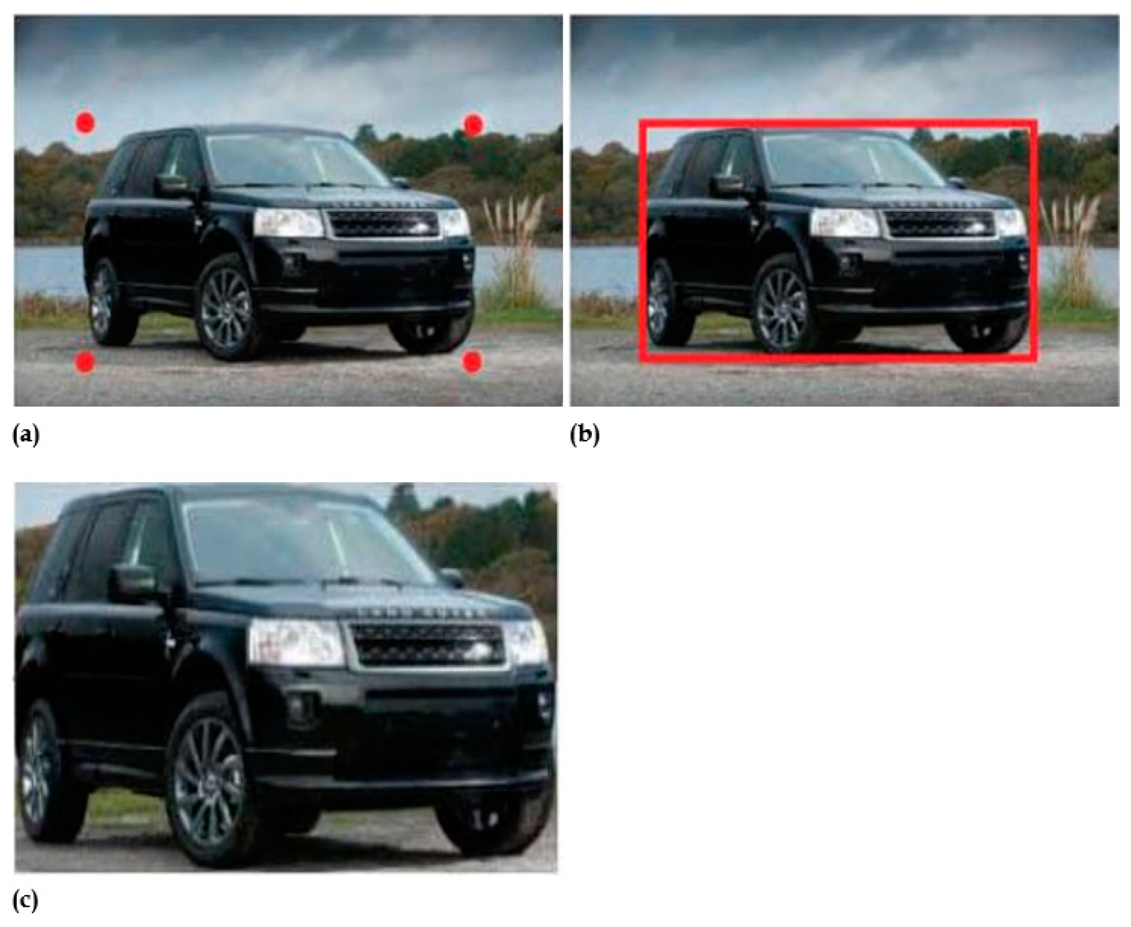
Images from the Stanford Cars and BMW-10 datasets were compiled and categorised according to the manufacturer and model of each car using the available MAT files. These datasets were created from web images, including images from Google, Amazon, Bing and other sources. Noise-free images were included in the dataset to ensure successful model training across various convolutional networks. The Stanford Cars dataset contained 196 car models of different makes, while the BMW-10 dataset contained 10 models of a single-make BMW. Generally, classes may be categorised as SUVs, Coupes, Hatchbacks, Pickups, Convertibles, Sedans and Station Wagons; however, in this study, classes were categorised on the basis of models. Both of the datasets contained train and test MAT annotation files, a cars meta (makes of cars) file, training and testing image names with the path available within the annotation file and the bounding box of each of the vehicles, which was accessible according to the image name. All of the images were cropped and organised into categories with the help of the bounding box points from the provided file. The processed images are shown in
Figure 10.
The PAKCars dataset is built from the most popular cars in Pakistan and can be used to improve the country’s traffic management system with more precise vehicle classification. It is a somewhat modest data set. Several photographs, taken from different view angles, are presented. In order to extract the dataset, authors cropped each image with the cropping tool and saved it to the appropriate class directory according to the make and model. This ensured that the images were solely focused on the vehicles in the images. There were 40 different car types included in the dataset, all of which are common in Pakistan.
3.4. Dataset Augmentation
Dataset augmentation is helpful for CNN models because it can artificially increase the size of a dataset and thus help the model learn to recognize objects more robustly and better generalise patterns to new, unseen images. When a CNN model is trained on a dataset, it learns to recognise patterns in the images and makes predictions based on these patterns. However, if the dataset is small or limited in some way, the model may learn patterns that are specific to the images in the dataset but may not generalise well to new images. Dataset augmentation can help to mitigate this problem by creating new images from the original images, which can expose the model to a wider range of variations in the images. This can help the model learn to recognise objects more robustly and be less reliant on specific patterns in the images. Training the model on a larger and more varied dataset can reduce overfitting and make the model more robust for use with unseen data [
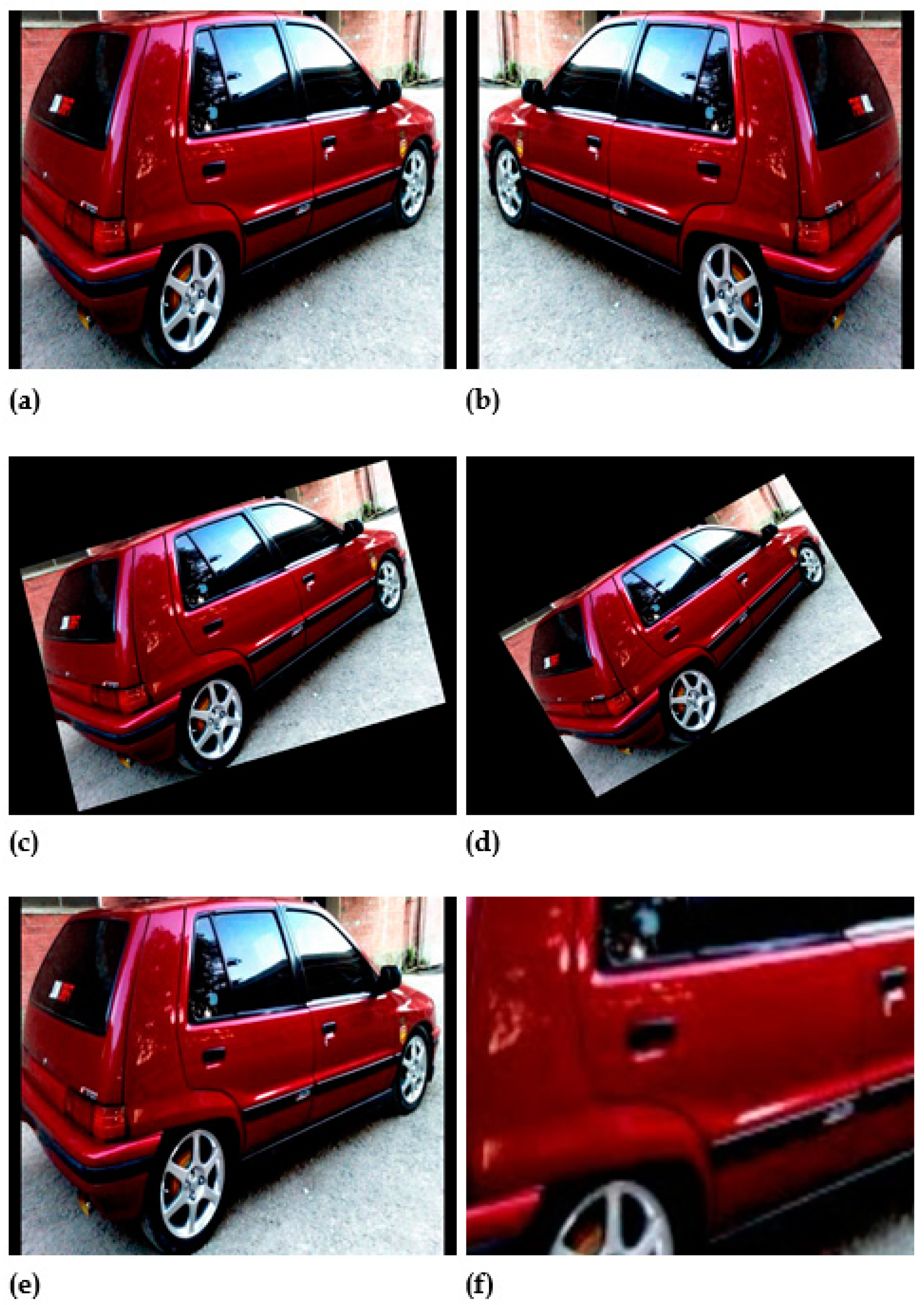
20]. The procedures for basic augmentation are incredibly simple. On any sort of image dataset, these strategies can be easily deployed. The following are some of the most common basic techniques used for data augmentation, as shown in
Figure 11:
Flipping
15-Degree Rotation
30-Degree Rotation
Zooming
Scaling
Cropping
3.5. Model Selection
It is important to identify which model will perform better for image classification tasks in supervised machine learning. There are two types of supervised machine learning models available: (1) Traditional models (support vector machine, decision tree, K-nearest neighbour, etc) and (2) CNN-based models (vgg, resnet, inception, mobilenet, alexnet, etc). Despite having several shortcomings, the conventional machine learning image classifi-cation approach has a number of benefits in raising the efficiency of picture classification. Traditional models lose their classification accuracy when working with large datasets and require a lot of computing effort. Over traditional models, convolution neural networks provide remarkable improvements in the recognition and classification of image features [
21]. The four most widely used models, mobilenet-V2, inception-V3, vgg-19 and resnet-50, were chosen for fine-grained vehicle classification tasks while keeping in mind all of the characteristics and performances reported in previously available research.
3.6. Training Process
Fine-grained vehicle classification was implemented using four different DCNN models on three datasets, with pre-trained models used as a starting point rather than starting from scratch. This had several advantages. The pre-trained models were already trained on a large dataset (ImageNet) that contained 1.2 million images classified into 1000 classes. Pre-trained model weights were utilised to train the DCNN models on the given datasets. The reason for this is that the model’s initial layers included edge and shape detection modules, which are common for any image recognition application, and these become increasingly abstract in the final layers, making them more application-specific. The learning rate of the plan was rooted at 0.001 to attain a network that was fine-tuned. After each batch of training sets, the learning rate was reduced by a very small factor of 0.000001; the purpose was to reduce the learning rate and provide better training to models on the given datasets. To evaluate the loss, cross-entropy was utilised; the function of loss was inversely proportional to the momentum. The model was trained with a stochastic gradient descent (SGD) optimiser with a learning rate of 0.001 to 0.000001 and augmented datasets were used instead of the original dataset to avoid model over-fitting. Cropping, scaling, rotating, flipping and zooming are some simple augmentation techniques that were used in this study to make the model more robust and avoid over-fitting.
3.7. Testing Process
In the testing process of fine-grained vehicle classification, the testing dataset was used as an input of ConvetNet models to predict classes and check the model accuracy. If the model accuracy was not satisfied, we made some changes to the training algorithm and dataset, including or excluding numbers of layers scratched on the CNN model, fine-tuning the hyper-parameters and dataset augmentation. This cycle was repeated if the results were not satisfying.
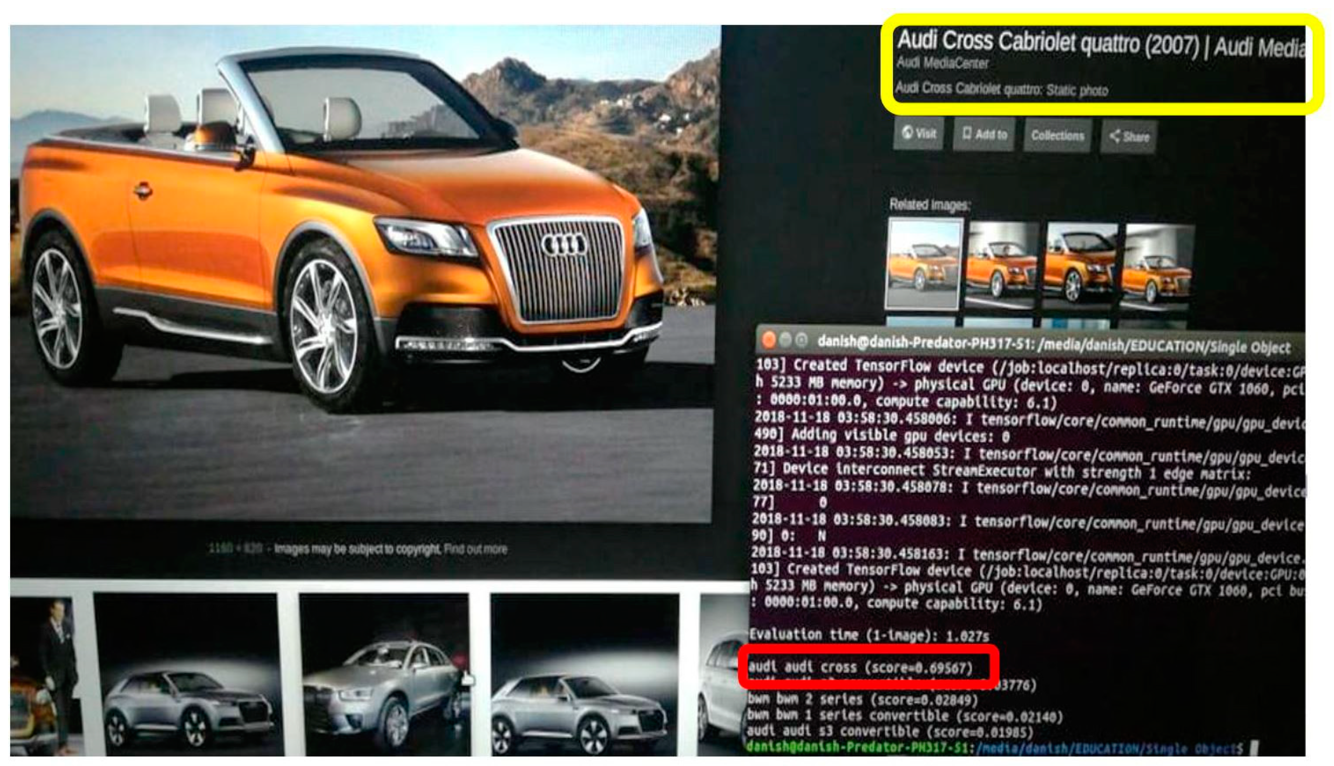
Figure 12 shows the testing of the trained model in which a new image from Google was provided as an input to the model and a prediction of the model is shown.
3.8. System Setup
Well-known deep convolutional network models were used in this study to solve the fine-grained vehicle classification problem. The majority of the models (Inception, Resnet and VGG) were winners of the ImageNet challenge. Since deep convolutional neural networks are computationally complex, they require a high-configuration processor. For this, a Core i7-powered, 16 GB RAM-equipped and 6 GB Nvidia GTX 1080 graphics capable Acer Predator Helios 300 laptop was used. The following is a list of the major toolkit components used in this work:
Ubuntu 16.04.
Python 3.7.
DCNN library Tensorflow and Mxnet.
For GPU, CUDA 8.0.4 was used.
CUDN was used to run faster computations of CNN models.
4. Results and Discussion
The experimental findings of the implemented DCNN models on each dataset are shown in
Table 2. This study made use of three independent car classification datasets (BMW-10, Stanford Cars and PAKCars) for fine-grained categorisation. Several researchers have used the BMW-10 and Stanford Cars datasets to train multiple DCNN models. In
Table 3, the results of this investigation are compared to those of earlier studies. In [
22], researchers employed between 50,000 and 250,000 epochs with fine-tuned parameters. In this work [
23], Keras library was utilised for data augmentation and model training, giving results comparable to our work but with slightly higher accuracy. However, our proposed method of augmentation has been shown to produce better results and has the added benefit of reducing the training time by generating fewer augmented images. This makes it an attractive option for those seeking to optimise their model training process. Additionally, the dataset split in this study was 50/50 for the training and testing sets. The performance of the mobilenet-v2 model could not be compared to any other study because the implementation of the fine-grained classification of vehicles was not found in any further study. The implemented model’s work was only trained for 100 epochs (ResNet and VGG) and 20,000 epochs (Mobilenet and Inception-V3) due to hardware limitations and this is comparable with previous studies. In the future, it will be possible to engage in training with additional epochs to better appreciate the usefulness of each model and improve performance.
Test Images
We tested a trained model with the generated test dataset and the result was quite promising; the confidence of the applied trained models on all sample test dataset images of the three datasets (Stanford Cars, BMW-10 and PakCars) had an accuracy of up to 87%.
Table 4,
Table 5,
Table 6 and
Table 7 show the prediction output of all models on the test set.
5. Conclusions
Fine-grained vehicle classification is an important component of ITS, which encompasses a wide range of technologies and applications related to the efficient and safe management of transportation systems. By demonstrating the effectiveness of CNNs for fine-grained vehicle classification, this work contributes to the development of more advanced and intelligent transportation systems. The results of this study could be useful for practitioners seeking to develop applications related to fine-grained vehicle classification, such as traffic management, surveillance and prediction systems. The comparison of different CNN models and analysis of trade-offs between accuracy and model size are useful contributions to the machine-learning community as they provide a deeper understanding of the capabilities and limitations of these models for fine-grained vehicle classification. The proposed data augmentation algorithm could be useful for practitioners seeking to optimise the training process for CNN models. Four different models were chosen for this study and implemented on three different datasets to analyse the performance of the CNN models. First of all, mobilenet-v2 was tested, which gave a low output percentage compared to the inception-V3 model. Then, the vgg-19 model was tested, which provided better testing predictions compared to the mobilenet-v2 and inception-V3 models. However, the best model found in this study was the residual network model (ResNet-50), which gave the best predictions for testing data but had a higher loss function. Although, the overall performance of resnet-50 was the best among all. In the case of BMW-10 and Pak-Cars, vgg-19 performed a little better than resnet-50. It was concluded that resnet-50 leads to faster convergence and better prediction results compared to the other models. Significantly, the above conclusion is not final, as some other models could also be tested. Better results could be achieved by using proper resources and overcoming limitations. However, the deduction obtained from this research was very substantial and proper inferences can be obtained to decide upon the best model. In our case, the overall performance of resnet-50 was better but, in some cases, vgg-19 produced better results. In the future, traditional models and other DCNN classifiers can be implemented and compared. In addition, other large-scale vehicle datasets (Boxcars, BRCars, etc.) can be utilised to evaluate the diversity of models for the fine-grained classification of vehicles. Many improvements can be made with further research and analysis.


