
Simulative Study of an Innovative On-Demand Transport System Using a Realistic German Urban Scenario


Department of Mechatronics, University of Duisburg-Essen, 47057 Duisburg, Germany
*
Author to whom correspondence should be addressed.
Future Transp. 2023, 3(1), 38-56; https://doi.org/10.3390/futuretransp3010003
Submission received: 20 September 2022
/
Revised: 14 December 2022
/
Accepted: 27 December 2022
/
Published: 30 December 2022
(This article belongs to the Topic Transportation in Sustainable Energy Systems)
Abstract
:Trams are a meaningful means of public transport in urban traffic. However, trams have some well-known disadvantages. These include, for example, possibly long distances to the stop, long waiting times, and lack of privacy, among others. The innovative mobility concept “FLAIT-Train” offers solutions to the problems mentioned. The FLAIT-train operates on ordinary roads and is intended to offer DOOR-2-DOOR transport. In the first application phase, the FLAIT-train runs on exclusive lanes but in the future can mix with other traffic. They are designed as vehicles with 2 seats and 1 m width. The vehicle technology of FLAIT-trains is similar/identical to battery-electric autonomous vehicles. This paper uses traffic simulations to investigate whether FLAIT trains are a suitable alternative to conventional trams, taking simulated/theoretical transport capacities in passenger-kilometers per day into account. Using the software SUMO (“Simulation of Urban Mobility”), a realistic traffic scenario is generated. In this scenario, the operation of the FLAIT-Trains and the trams are simulated under the same conditions and based on statistical data. Based on the simulation results, the performances of the FLAIT-Trains and the trams are compared.
1. Introduction
The rail-bound metro and tram offer many economic and ecological advantages as meaningful means of public transport. In particular, they contribute to improving sustainability and quality of life in urban areas [1].
However, these rail-based modes of transport have some well-known problems that strongly affect their acceptance. For one, poor accessibility to fixed stops prevents better attractiveness of trams [2]. Passengers must often walk long distances and sometimes even cross several streets to reach a stop.
Another optimization potential of rail-based modes of transport is the total travel time. The total travel time includes the walking time to the boarding stop and from the alighting stop to the destination, the waiting time at the stop, and the effective travel time. For rail-bound trams, the average waiting time is approximately equal to half the tram cycle time, according to [3]. The in-vehicle time of trams can also be optimized by reducing the intermediate stops, including boarding and alighting times.
Furthermore, the privacy of every passenger in a tram cannot be ensured, e.g., when talking to fellow passengers or talking on the phone. Studies like the one by [4] show that the comfort of tram travel is often not perceived as satisfactory due to the limited number of seats and the bad air during rush hours.
The classic metro and tram also have numerous operational and economic problems. According to [5], the investment costs for infrastructure amounted to 12 M€/km in 2008. Furthermore, the high inspection costs and the large surface area occupied by the separate rail areas also count as operational problems for urban rail vehicles.
2. Related Work
The on-demand transport systems have been studied together with the dial-a-ride problem (abbreviation: DARP). The DARP represents passenger transportation between paired pickup (origin) and delivery points (destination) and has been researched for over five decades [6,7]. According to [8], Dial-a-ride services may be provided in a static or a dynamic mode. In a static mode, all transportation requests are known in advance. In contrast to the static mode, requests are revealed, and vehicle routes are adjusted in real-time [8,9] in a dynamic mode.
Furthermore, the cases of DARP can be divided into single-vehicle and multi-vehicle DARP [8]. The first case describes the simple cases of the DARP, where all passengers are transported by a single vehicle. The single-vehicle DARP can also be denoted as SDARP [6].
Besides DARP, another alternative on-demand transport system, Personal Transit System (abbreviation: PRT), has also been researched [10,11]. The PRT is an automated transit system and driverless. The PRT is a fixed network, including dedicated off-line stops. Because of the smaller vehicle size (2 to 4-person vehicles) and its on-demand technology, the PRT system can provide passengers with faster travel time by saving intermediate stops [10]. According to [11], the major differences between PRT and other transport systems include, e.g.,
- the PRT traffic does not interfere with other traffic participants, because the PRT track is elevated to a higher level or hidden underground;because of the separation of the track from pedestrian traffic, the PRT system provides a high-level of safety. However, the investment costs for the infrastructure of PRT systems amounted to 30–100 M$/Mile, according to [10], because of the exclusivity and technical complexity of PRT tracks.
2.1. Scientific Research of DARP
Since the first DARP service in 1970, numerous research regarding models and algorithms of the DARP has been published. The publications and developments up to 2007 have been summarized and described in [12]. The more recent research until 2018 has been introduced in [7]. The publications until 2021 have been summarized by [13].
The first models regarding the planning and scheduling of DARP have been presented in [14]. Since then, the research for different cases has been studied continuously. As noted in [12], two possible problems have been considered in the publications: (1) minimize costs subject to full demand satisfaction and side constraints; (2) maximize satisfied demand subject to vehicle availability and side constraints. E.g., the fleet size, operation costs, and driver’s wages belong to the common costs and side constraints. The common demand satisfaction relates to the customer waiting time, in-vehicle time, or route duration.
In [15], the single-vehicle case in static mode was analyzed and solved as a dynamic program in 1980 to minimize a combined objective function of the route duration, the total waiting time, and the in-vehicle time of all passengers. In parallel, research on the same problem has also been conducted using Benders’ decomposition procedure [16,17]. Further research solved the single-vehicle DARPs using different approaches. The DARP has been handled as a k-forest problem to optimize the total routing distance [18]. In [19], the cost-effectiveness of a single-vehicle DARP and the total travel distance have been optimized using some metaheuristic techniques, such as Simulated Annealing, Generic Algorithms, Particle Swarm Optimization, and Artificial Immune System.
Since the research in [20], most publications have focused on developing the multiple-vehicle DARPs. They were distinguished majorly by different constraints and objective functions. While some of them minimize the travel costs, including, e.g., total ride distance and duration, with the assumption of an efficient number of available vehicles [21,22,23,24], some researchers maximized the service quality measures using a limited number of available vehicles [25,26,27]. Furthermore, some publications took vehicle emissions into account [28]. The passenger occupancy rate [29], service provider’s operational costs and profit [30,31,32], workforce planning as well as staff workload [33], and system reliability [34] were also among the objective functions considered. The detailed introduction and classification of different models and algorithms are referred to in [7,12,13].
2.2. Application Projects of DARP in Germany
In North and South America and Asia, ride-hailing services are the most popular on-demand mobility services, dominated by Transportation Network Companies like Uber, Lyft, or DiDi. As introduced in [35], ride-hailing services are not common in Germany due to strict regulations. Instead, some on-demand mobility services in the form of ride-pooling have been provided. Some of them have been provided by private enterprises (Start-ups) like MOIA in Hamburg and Hannover since 2019 and 2017, respectively [35], CleverShuttle in Munich, Leipzig, Hamburg, and Berlin [36], Allygator Shuttle in Berlin, ioki in Frankfurt [37]. There are also some services which have emerged through the cooperation of municipal transportation companies and start-ups. Examples are the LüMo in Lübeck, myBus in Duisburg, SSB in Stuttgart, and Berlkönig in Berlin [37]. In addition, a service called “Bedarfsbus Schorndorf” has been provided by a research project [38].
3. FLAIT-Trains
The innovative concept “Fast Lane AI Transportation Trains (FLAIT-Trains)” [39] offers a solution to the problems mentioned above. The FLAIT-Trains consist of individual FLAIT vehicles. The final target of this concept is to provide the DOOR-2-DOOR service using fully autonomous FLAIT vehicles. The FLAIT-Trains drive mixed with other traffic participants, e.g., personal cars, bicycles, etc. Because of the limited available technologies, the final target will be achieved step by step. An intermediate solution of FLAIT-Train will be introduced and studied in this paper.
In this step, the focus of the FLAIT-Train research is the analysis of the replacement possibility of the conventional trams. One constraint of this intermediate solution is that the FLAIT-Trains will use the same track area as the trams (same space requirement). As the second constraint, the routes of the FLAIT-Trains are predetermined. The considered FLAIT is designed as a highly autonomous battery-electronic vehicle. Due to this design, a FLAIT runs without local CO2 emissions and thus retains the exhaust gas advantage of the tram. Because this design enables the vehicle to be controlled without a driver or driver-relevant components, the compact external dimensions and lower weight of the FLAIT are feasible.
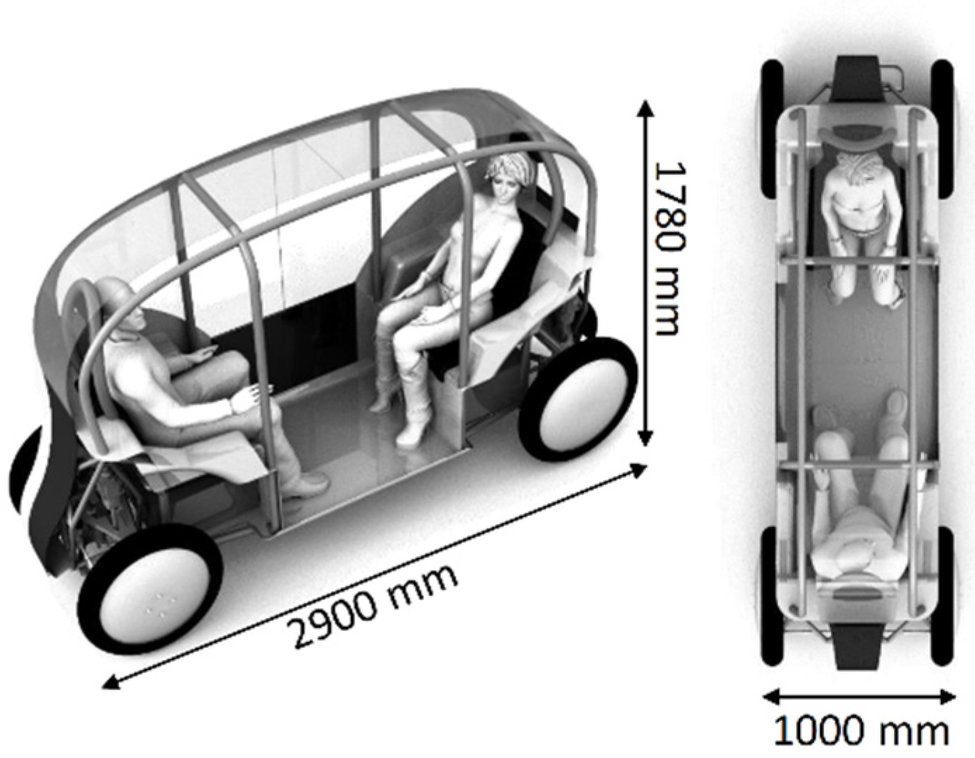
Similar to a PRT vehicle, a standard FLAIT vehicle is designed for a passenger capacity of two people. On the one hand, this number fits the average passenger car occupancy rate of 1.5 [40]. On the other hand, seating comfort and privacy are ensured for all occupants. Due to the small passenger capacity, the number of stops to the destination is also reduced. Thus, passengers save travel time with the help of FLAITs. Another advantage of the limited number of passengers is the possible narrow FLAIT vehicle width of one meter. This narrow body allows two FLAITs to travel side by side on the roadway with a width of the classic tram track. Figure 1 shows the vehicle dimensions of a FLAIT.
To realize highly automated driving, FLAITs are equipped with appropriate sensor technology (see Figure 2). For example, via detection by camera or sensors of fixed known and measured “landmarks” (e.g., lantern, bus stop shelter, traffic light, etc.), the FLAITs can be guided along a predefined route. In addition, a camera or a similar sensor can also be installed in the upper area of the FLAIT. This allows a FLAIT to detect preceding FLAITs within the sensor’s range. Based on this sensor technology, the FLAITs can form flexible platoons, thus saving occupied spaces, especially during rush hours.
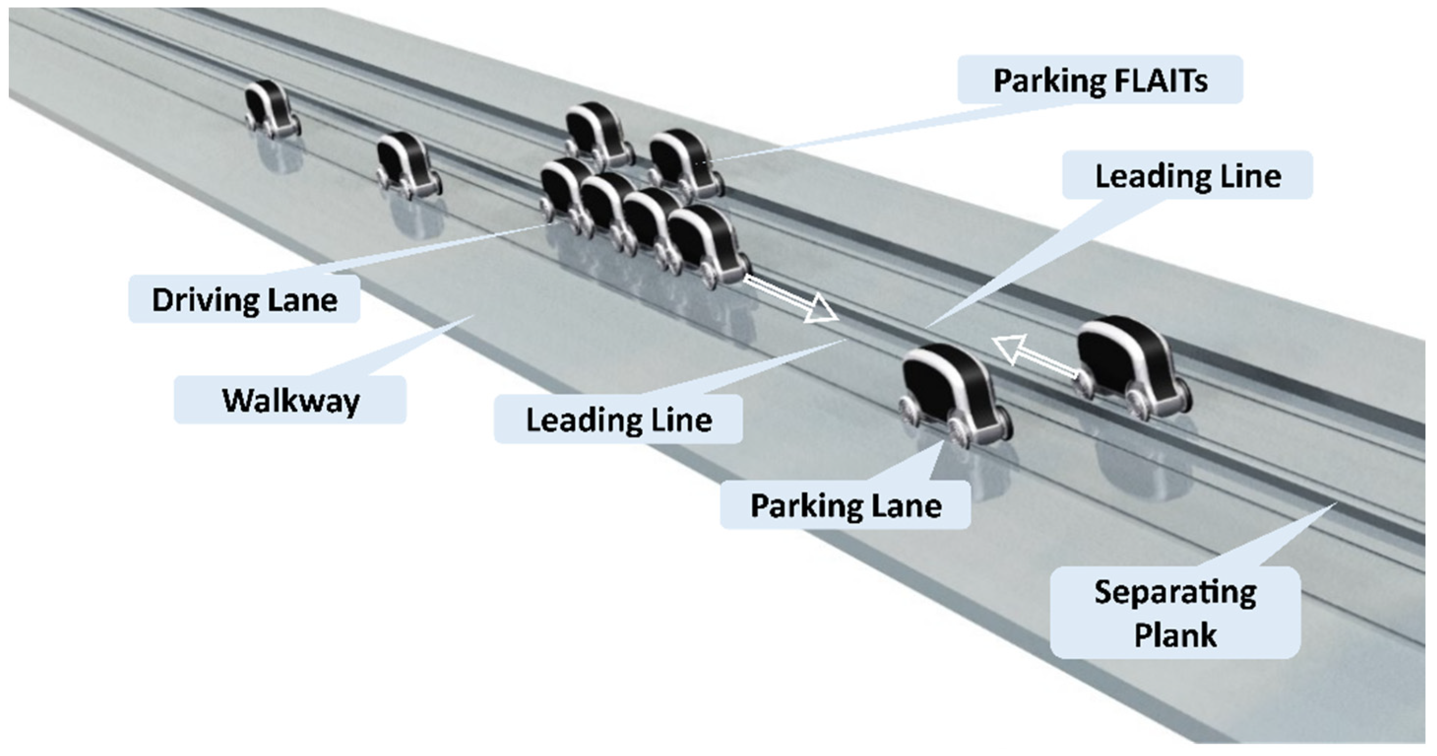
Figure 3 shows a FLAIT train system based on the above vehicle design. In each direction of travel, the width of the classic tram track is divided into two lanes: the driving, and the parking lane. On the parking lane, a FLAIT can stop at any point without blocking the traffic of the FLAITs behind it. Due to the fully autonomous control, the FLAIT journeys no longer depend on the drivers’ working hours. A passenger can reserve a FLAIT anytime via smartphone or other mobile devices. The passenger waits for the FLAIT directly at the parking lane and does not need to walk to the fixed stop. This reduces the waiting time and the walking distance to the stop. The FLAIT system’s advantages are summarized and illustrated in Figure 4. Based on the comparison table in [7], the characteristics of FLAIT-Trains have been complemented in Table 1.
4. Methodology
4.1. Aim and Key Figures
Due to the limited passenger seating capacity of each FLAIT, it is necessary to check whether a reasonable number of FLAITs can cover the system performance of the classic metros and trams. According to [44], transit system performance is defined as the composite measure of transit system operating characteristics, primarily quantitative, such as service frequency, speed, reliability, safety, capacity, and productivity. Especially during rush hour, there is a maximum value of the passenger volume. FLAITs must ensure that all passengers are transported to their destination with comparable or less waiting times. In addition, the required number of FLAITs must be determined by simulation. Based on this result, it is analyzed whether the resulting number of FLAITs can be considered for operational and economic reasons. In the real FLAIT-Train system, the passengers can board and alight at every point of the FLAIT tracks without fixed stops. However, this paper aims to check whether the FLAIT-Trains can carry all passengers transported by trams in the available statistical data.
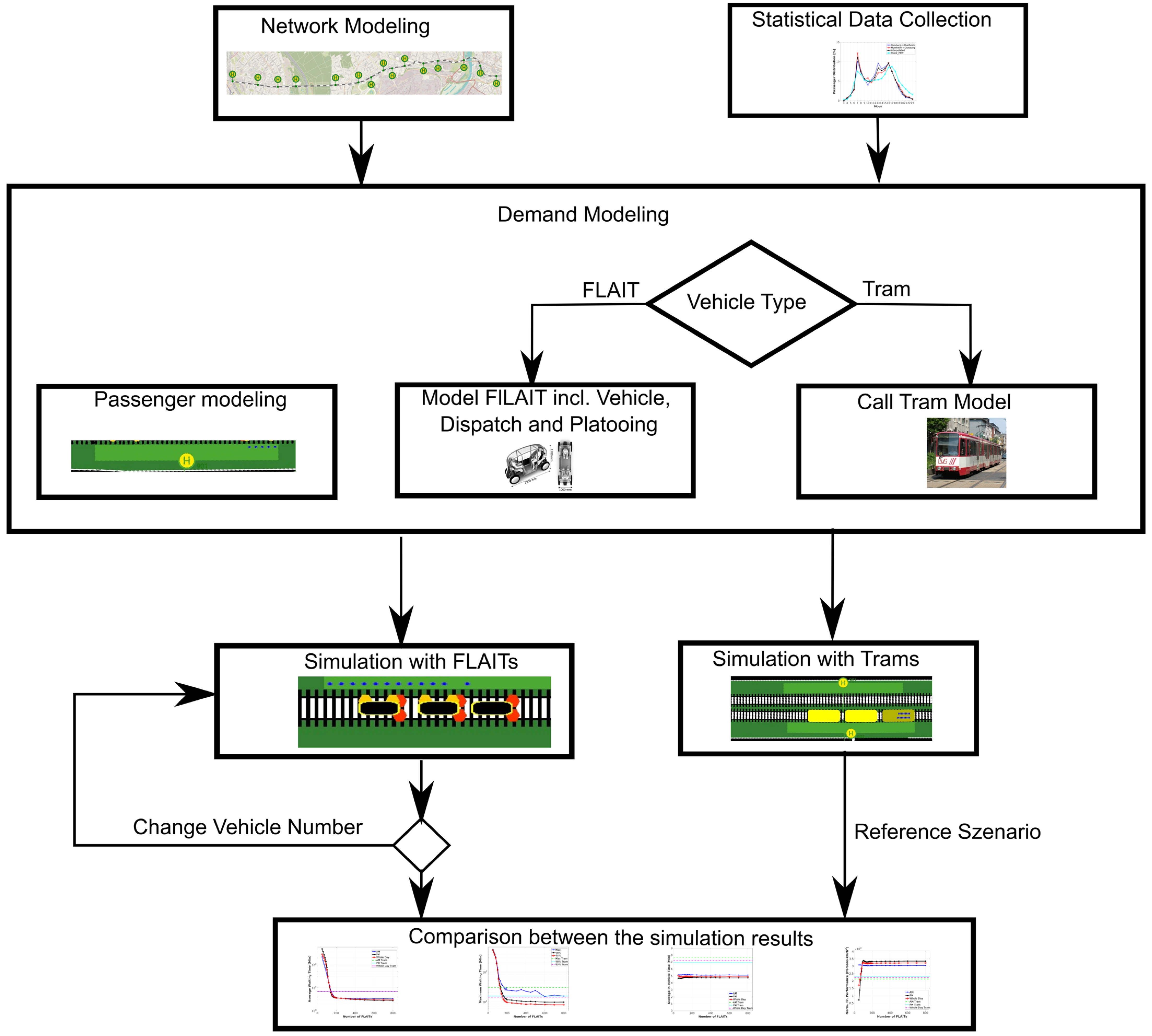
For this reason, the passenger in the simulation with FLAIT-Trains will still be picked up from the tram stops. Therefore, this paper does not consider the influence of the flexible stop of FLAIT. The methodology is described graphically in Figure 4.
The evaluation of the system performance is based on the following five key performance indicators:
- average waiting time per passenger,
- maximum waiting time for a single passenger,
- average in-vehicle time per passenger,
- daily transportation productivity, and
- total annual service provider’s costs.
4.1.1. Average Waiting Time per Passenger
Because the average waiting time per passenger is a critical metric representing public transport service reliability [3], this metric is an important evaluation criterion in this paper. The average waiting time per passenger results from the mean value of the waiting times of all passengers:
The parameter stands for the waiting time of the -th passenger and for the total number of passengers transported.
4.1.2. Maximum Waiting Time of a Single Passenger
For on-demand public transport, the maximum waiting time of a single passenger is also an important indicator of service quality, in addition to the average waiting time [45,46]. For this reason, this paper also considers this indicator. The maximum waiting time of a passenger represents the longest time a passenger has to wait at a stop. This key figure is determined by
4.1.3. Average In-Vehicle Time per Passenger
The average in-vehicle time per passenger represents the pure journey time by tram or FLAIT and was considered in [3] as an essential assessment factor of public transport service reliability. In this paper, this metric is derived from the formula
Here stands for the in-vehicle time of the -th passenger with the corresponding vehicle.
4.1.4. Daily Transportation Productivity
In order to compare two transit systems, tram and FLAIT-Train, a performance measure from [44] is applied in this paper: daily transportation productivity . This indicator is derived from transportation work . According to [44], transportation work is defined as the quantity of the performed movement and computed as the number of transported objects multiplied by the distance over which they are carried. The transportation work performed per unit of time represents transportation productivity. In this paper, the daily transportation in the unit: is determined using the formula
The individual transport performance of each passenger results from the formula [47], where stands for the traffic volume, for the length of the transport route, and for the transport time or journey time. For each passenger, the traffic volume is equal to 1 person. For this reason, the total traffic line was determined using the formula
4.1.5. Total Annual Service Provider’s Costs
To determine the suitable number of the FLAITs, the total annual costs of the service provider have been applied as a key performance indicator from an economic point of view. As introduced in [48], following three service provider’s cost types have been taken in this paper into account:
- infrastructure costs (Cin),
- vehicle costs (Cveh), and
- operating costs (Cop).
The annual infrastructure costs have been calculated as the annual depreciation amount value using the formula
where stands for the total infrastructure investment and for the lifetime.
The annual vehicle costs have been determined according to the formula
where denotes the costs per vehicle, for the lifetime of the vehicles and for the size of the vehicle fleet.
The annual operating costs have been calculated assuming a linear dependency of the size of the vehicle fleet and according to the formula
where denotes the annual operating costs per vehicle.
The total annual service provider’s costs equal the sum of annual infrastructure, vehicle and operating costs and have been calculated by
4.2. Simulation Scenario
4.2.1. Tram Route between Duisburg Central Station and Mülheim Central Station
In the context of this paper, the tram route of line 901 between Duisburg central station and Mülheim central station is considered. This line is one of the most important tram routes in both cities. Duisburg and Mülheim/Ruhr each have 501,591 (as of 30.06.2020) [49] and 172,717 (as of 31.12.2021) [50] inhabitants, making them the fifth and eighteenth most populous cities in the federal state of North Rhine-Westphalia. This route connects the main stations of both cities and landmarks, such as the University of Duisburg-Essen, Duisburg Zoo, Broich Castle, and the Ruhr West University of Applied Sciences. For these reasons, it is one of the busiest public transport routes in Duisburg and Mülheim/Ruhr.
The tram route under consideration has a total of 16 stops, as shown in Figure 5. The outward journey from Duisburg Central Station to Mülheim Central Station takes 21 min per the timetable [51], while the return journey takes 22 min.
Simulations with different numbers of FLAITs were carried out to show the influence of the number of FLAIT vehicles on transport performance.
In parallel, a reference simulation in the same scenario with trams was also carried out. In this reference simulation, the actual timetables have been used.
4.2.2. Relevant Vehicles
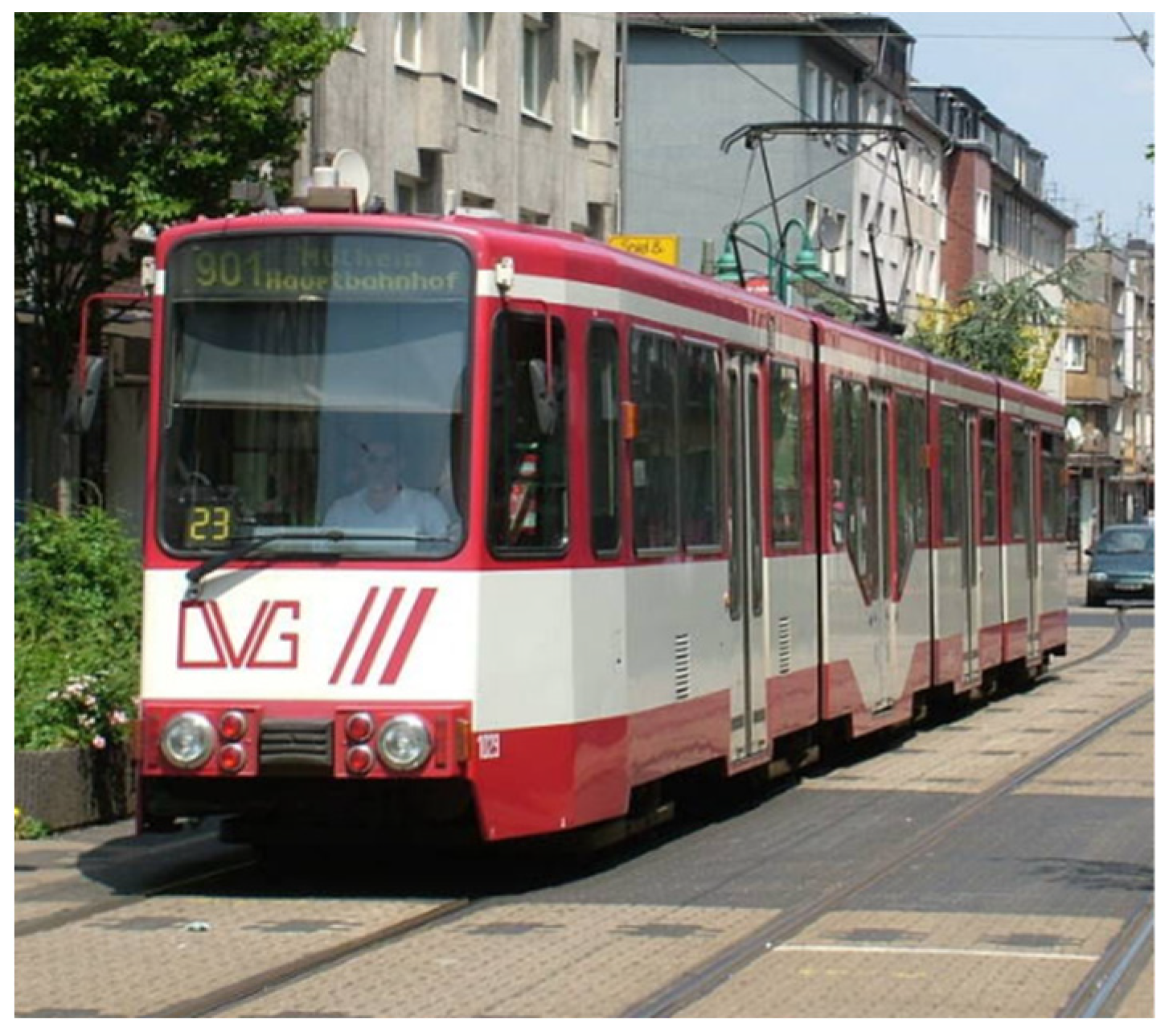
For the simulations, trams and FLAITs were modeled. The tram “DVG GT-10 NC-DU” (Figure 6) was considered in the context of this contribution, which is currently used for line 901 in Duisburg. Thanks to the support of the DVG (Duisburg Transport Company), the parameters of this tram were made available. The important parameters of the vehicles are listed in Table 2. For the FLAITs, in addition to the parameters in Chapter 2 and Table 2, the demand-driven reservations and the flexible platooning must be modelled as vehicle characteristics of the FLAITs and represented during the simulation.
4.3. Modelling and Simulation
To simulate the above scenario with the classic trams and FLAIT trains, the open-source microscopic traffic simulation software SUMO (Simulation of Urban MObility) was used. According to the requirements for the simulations and the conducted analyses of different simulation software [53,54], SUMO was chosen as the simulation software for the use cases of this contribution.
4.3.1. Vehicle Models
Tram
In SUMO, the existing vehicle class “Tram” was used to model and simulate trams. The parameters from Table 1 replace the default parameters in source code. Because an urban scenario was considered, the driving speed of the tram model was limited to 50 kph, as it is the maximum speed allowed in German cities.
FLAIT
The FLAIT vehicles were modeled as a new vehicle class, “Flait” in SUMO. The modeling combined the existing models of trams and taxis in SUMO. As a replacement for trams, the FLAITs are only allowed to drive on the tram tracks (SUMO road type “railway.tram”). The FLAITs stop at the last exit point of the passenger and only start again when the next passenger reservation arrives. As with the tram modeling, the travel speed of the FLAITs was limited to 50 kph within the scope of this contribution.
4.3.2. Passengers
In the simulations, different passenger groups were modeled using the SUMO function “personFlow” [55]. For each group, are given as parameters. Because transport performance is the focus of this paper, passenger walking distance and time were not considered as criteria. For this reason, passengers were assumed to send out the FLAIT reservations at the tram stops.
- the time to the second when the first passenger of this group departs;
- the to-the-second times until when the last passenger of that group departs;
- the number of group members;
- the street ID where the group departs;
- the stop where the group waits for tram or FLAIT train;
- the destination street ID where the group alights
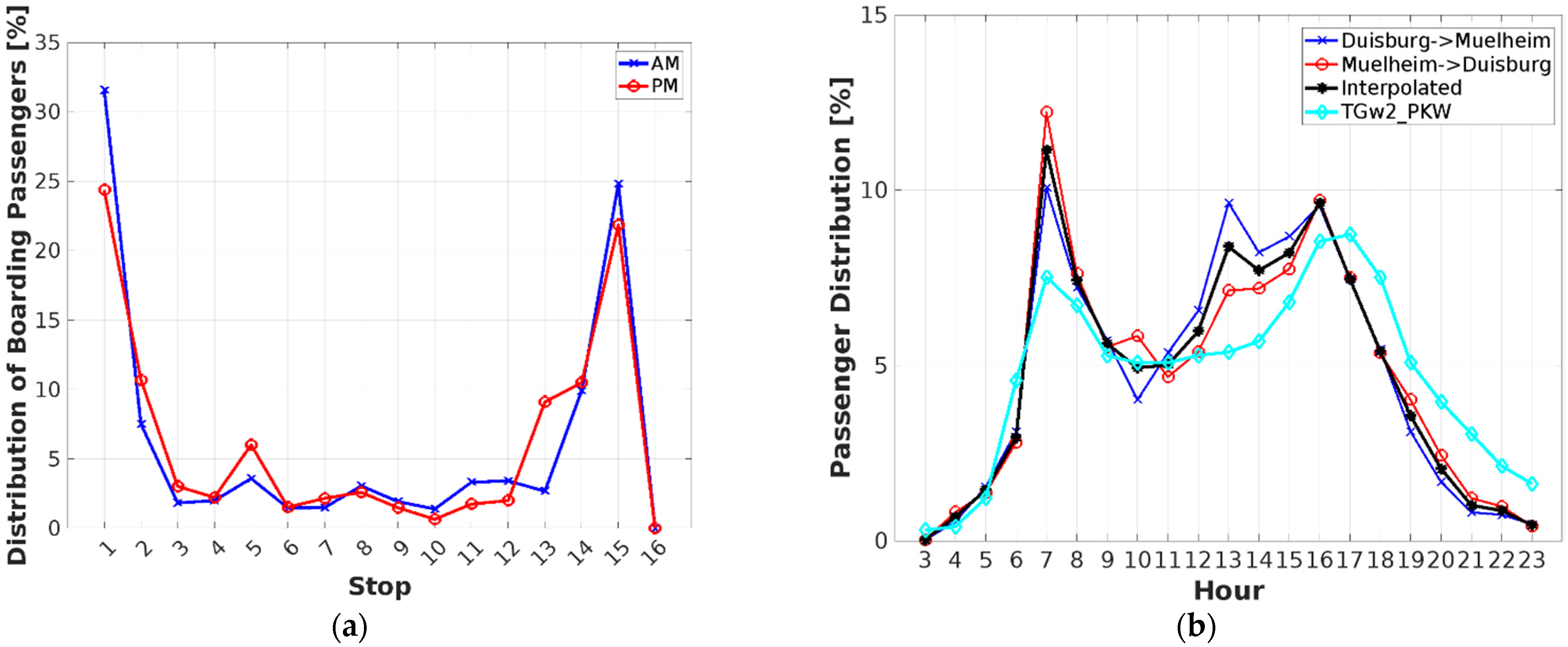
To make more realistic comparisons, some passenger statistical data have been provided by the DVG (Duisburger Verkehrsgesellschaft AG). According to these statistical data, the detailed passenger numbers of tram line 901 on a typical working day in 2018 are available. The statistics have not been affected by the COVID-19 pandemic and represent the typical traffic load of tram line 901. In Figure 7, the statistics from DVG are analyzed and illustrated partially in comparison with available data in some literature.
Figure 7a shows the distribution of the counted boarding passengers at each tram stop in the driving direction from Mülheim/Ruhr to Duisburg. According to the statistics, the most passengers have been boarded at the tram stops “Mülheim main station” and “Luther square”, in each case 31.56% and 24.81% of all boarding passengers in the morning (from 3 a.m. to 12 a.m.) as well as 24.37% and 21.86% in the afternoon (from 1 p.m. to midnight) correspondingly.
Necessary data for the traffic capacity analysis of public transportation are the hourly passenger distribution because the number of boarding passengers during rush hours is the decisive factor for the necessary vehicle numbers and their required cycle time. In the literature, no directly applicable distribution data was available, which have been derived from the statistics. In [56], an hourly distribution of the complete passenger vehicles’ traffic of a typical workday (Tuesday–Thursday) in the west German urban area is available, as shown in Table 2 and Figure 7b in cyan in comparison with the statistics from DVG. Because the publication focused on passenger car traffic distribution, the cyan line shows a different behavior than the other lines derived from the public transport statistics.
In Figure 7b, the blue and red lines illustrate the timelines of the two driving directions (from Duisburg main station to Mülheim main station and vice versa) based on the DVG data. By calculating the mean values of these two lines, the second row in Table 3 was generated and illustrated in Figure 7b in black.
The demands for mobility generally seem to have remained similar in terms of quality over the years, with at most slight differences in the characteristics of the transportation means, which in the case of public transport in the evening and at night could also have something to do with availability. The peaks in the morning and at midday for public transport are probably due to schoolchildren, who do not have access to passenger vehicles, which is why the curve of TGw2_PKW is flatter there.
After the comparison, the timelines based on the statistics from DVG are better suitable to represent the realistic German urban scenario. For this reason, they are used in the simulations of this contribution.
4.3.3. Flexible Platooning
In SUMO, a toolbox, “Simpla” has been developed to simulate flexible vehicle platooning based on [57]. In the context of this paper, this toolbox was used. The Krauss model [58] was applied as the car-following model. Because the FLAITs are highly autonomized vehicles, the model of perfect drivers was used.
5. Results and Analyses
In the scenario presented in Section 4.2, daily transport using different transport means has been simulated. Apart from the simulation with the classic trams, simulations with different numbers of FLAITs, from 50 to 800 FLAITs, were carried out. Different delta values between the considered numbers were chosen for the simulations (from 50 to 200 FLAITs with a delta value of 10 FLAITs, from 200 to 500 FLAITS with a delta value of 50 FLAITs, from 500 to 800 FLAITs with a delta value of 100 FLAITs).
Because the passenger distribution, according to the analysis in Section 4.3.2, has some differences between mornings and afternoons, all simulation results from Figure 8, Figure 9, Figure 10, Figure 11 and Figure 12 are analyzed for mornings (trams in green, FLAITs in blue, 3 a.m. to noon), afternoons (trams in cyan, FLAITs in black, noon to midnight), and the whole day (trams in magenta, FLAITs in red, 3 a.m. to midnight) separately.
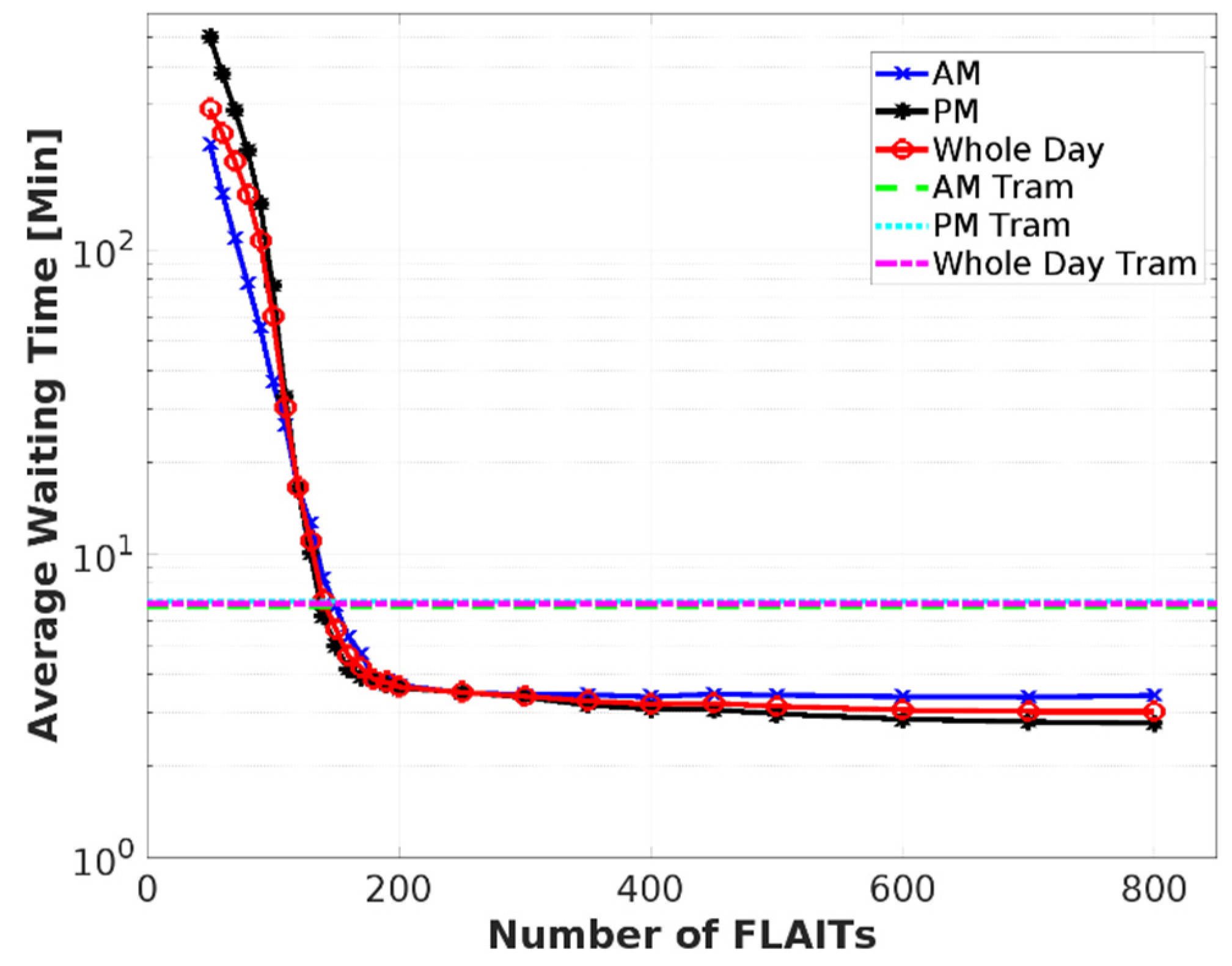
5.1. Average Waiting Time per Passenger
In the reference simulations with the tram, the average waiting time for mornings, afternoons, and the whole day was determined according to the formula (1) and showed similar values (respectively, 6.68 min, 6.95 min, and 6.85 min). For FLAIT-Train, the average waiting time presented the same dependencies on the FLAIT numbers in the mornings, afternoons, and the whole day, as shown in the logarithm scale in Figure 8. The simulation results for the whole day are analyzed as an example.
With 50 to 140 FLAITs, the average waiting times (respectively, about 291 min, 241 min, 195 min, 151 min, 107 min, 60 min, 30 min, 17 min, 11 min, and 7 min) were higher than the values for trams. With 150 to 180 FLAITs, this value was lower than the value from the reference simulation and decreased from 5.6 min, 4.6 min, 4,2 min, to 3.9 min. With 180 to 800 FLAITs, this value decreased from 3.9 to 3 min and changed significantly slower.
This effect is because, from a certain number of FLAITs, in this simulation from 180, at least one standing FLAIT is available for a future reservation. However, the further increasing number of standing FLAITs has no more influence on the average waiting time.
Compared to the trams, passengers can save 30% waiting time on average with 160 FLAITs. From 180 FLAITs, even more than 40% waiting time on average can be saved.
Figure 8.
Average Waiting Time per Passenger.

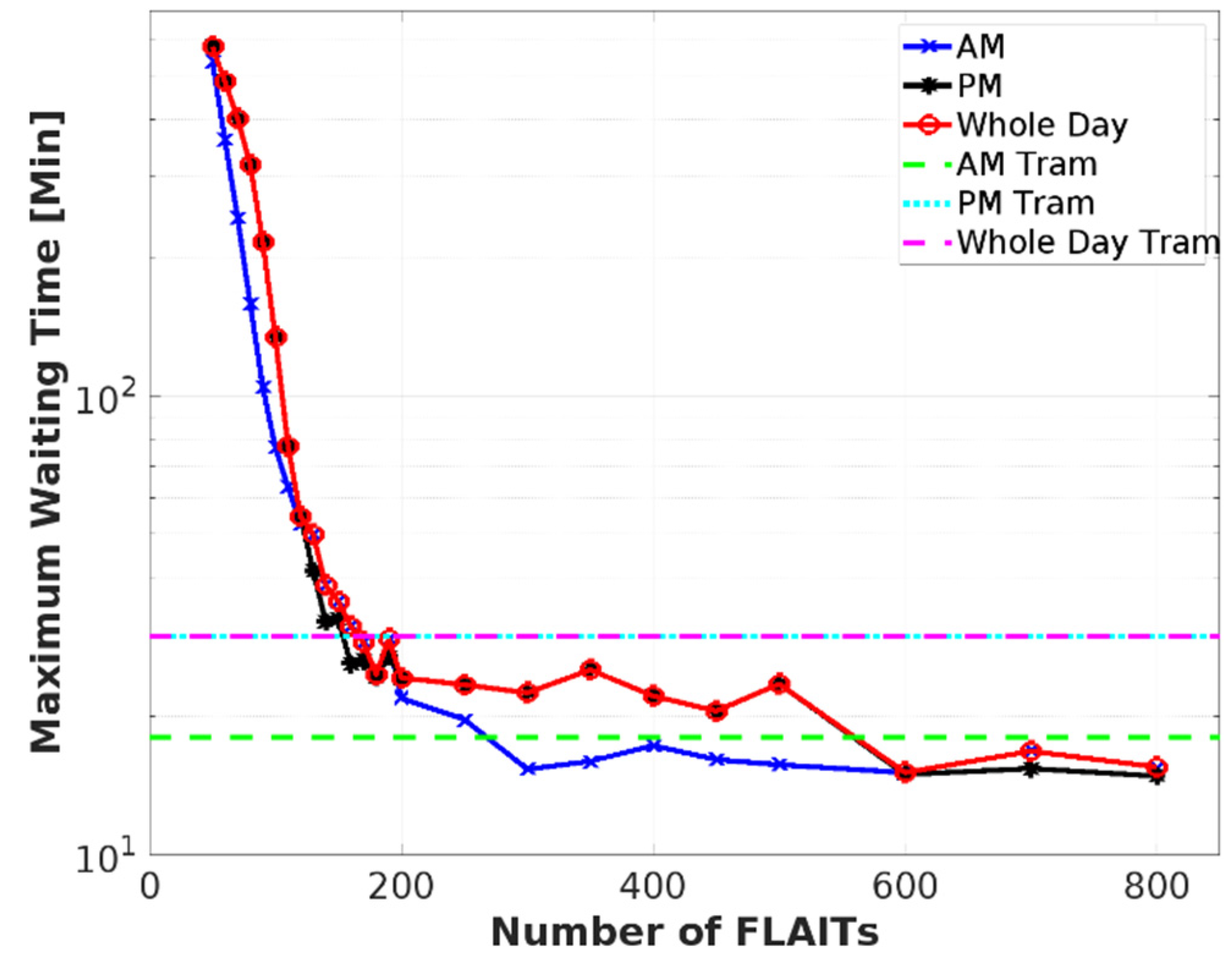
5.2. Maximum Waiting Time of a Single Passenger
In the reference simulation, the maximum waiting time of a single passenger riding a tram was determined using the formula (2) and was dependent on the timetable [51], about 18 min in the morning, 30 min in the afternoon, and on the whole day, respectively. Like the average waiting time, the courses of the maximum waiting time for FLAITs had similar dependencies on the FLAIT numbers in the three time periods, as shown in logarithm coordinates in Figure 9. The simulation results for the whole day are explained as an example in detail.
The values of this key figure from 50 to 160 FLAITs are higher than for the tram and are about 577 min, 484 min, 402 min, 319 min, 216 min, 134 min, 78 min, 55 min, 50 min, 39 min, 36 min, and 31 min, respectively. With 170 FLAITs and above, the values are lower than the reference value. With 800 FLAITs, a single FLAIT passenger could have a maximum waiting time of 16 min, and the relative saving compared to riding a tram is about 49%.
The maximum waiting time of a single passenger depends strongly on the applied dispatching algorithm. An unsuitable cost function considered in the dispatching algorithm could cause some single points with large maximum values. This paper used the dispatching algorithm integrated in SUMO without any optimization. In order to compensate for such impacts of the dispatching algorithm on the simulation results, the maximum waiting time of 98% and 95% of passengers were also analyzed, as presented in Figure 10.
The deviation between the values of absolute maximum in blue, the 98th percentile of passengers in black, and the 95th percentile of passengers in red was significantly recognizable already with 120 FLAITs (absolute maximum was about 55 min, maximum of 98% passengers was about 40 min and a maximum of 95% passengers was about 36 min). With 170 FLAITs, the maximum waiting time of 98% of passengers was about 15 min and already lower than the corresponding value for trams (about 16 min). With 200 to 800 FLAITs, the key figure decreased with a lower decreasing slope from 12 to 10 min, and the affected passengers saved from 25% to 38% waiting time compared to trams.
Figure 9.
Maximum Waiting Time for a Single Passenger.

Figure 10.
Analysis of the Maximum Waiting for a Single Passenger.

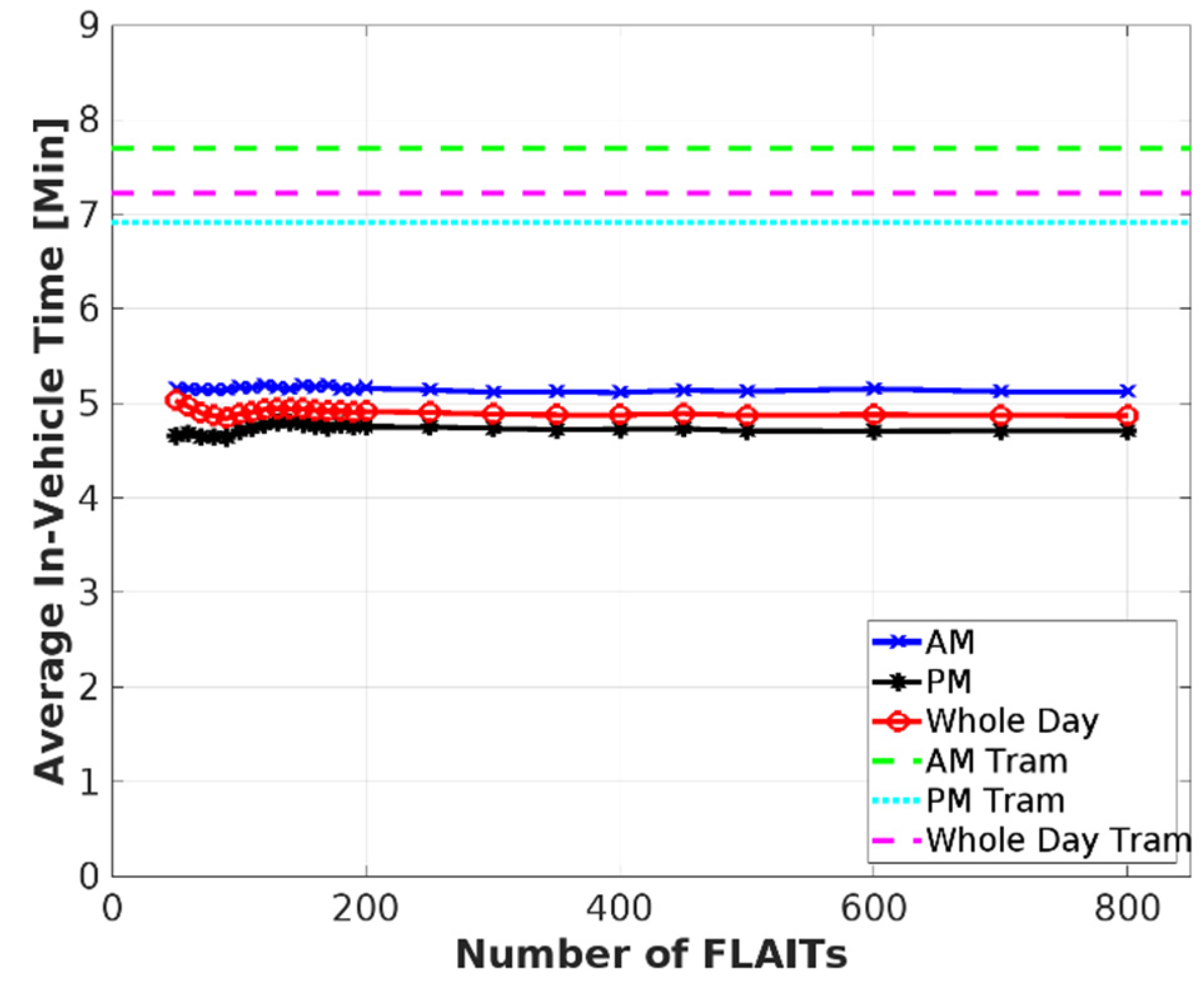
5.3. Average In-Vehicle Time per Passenger
Because the transport by FLAIT-Trains has no intermediate stops, the trip by FLAITs takes, on average, less time than the tram trips, regardless of the periods, as shown in Figure 11. According to Formula (3), the average in-vehicle time per tram passenger was determined. Depending on the departure and arrival stops, this resulted in about 7.7 min in the morning, 6.9 min in the afternoon, and 7.2 min for the whole day.
Compared to the reference values of the tram simulations, the trips of 50 to 800 FLAITs took between 5.1 and 5.2 min in the morning, between 4.6 and 4.8 min in the afternoon, and between 4.8 and 5 min. By saving the intermediate stops, a passenger saved about 32% of travel time in the morning, 30% in the afternoon, and 31% on the whole day.
Figure 11.
Average In-Vehicle Time per Passenger.

5.4. Daily Transportation Productivity
According to the timetable [51], the transport duration is 8.4 h in the morning, 12 h in the afternoon, and 20.4 h for the whole day. Correspondingly, the daily transportation productivity with trams determined according to Formula (5) is 511,146 persons∙km/day in the morning, 555,478 persons∙km/day in the afternoon, and 537,181 persons∙km/day on the whole day.
As presented in Figure 12, the simulation results with FLAITs showed some differences between the different periods. For this reason, the three time periods are analyzed separately in detail.
5.4.1. Mornings
Because all the passengers from the departure stops arrived in the morning were transported to the destination by FLAITs, the total transport performance in dependency of the number of FLAITs remained almost the same in a range between 724,937 and 741,735 (relative change lower than 2.3%) with 50 to 800 FLAITs. Due to less travel time, the values of FLAITs are higher than this key figure for trams. Compared to the reference simulation, the daily transportation productivity of FLAITs increased by more than 41.8%.
5.4.2. Afternoons
With 80 FLAITs and above, FLAIT-trains could show higher daily transportation productivity compared to trams (see Figure 12). From 50 to 100 FLAITs, the transportation productivity increased sharply and linearly with values from 172,219 to 811,771 persons∙km/day. From 100 FLAITs, this key figure ranged from 788,722 to 811,771 persons∙km/day and varied by less than 3%.
The curve has this behavior because all passengers, who waited at the stops, could not be transported to the target stop with less than 100 FLAITs until midnight. From 100 FLAITs, all passengers were transported to the target stops, and the further increasing number of FLAITs has no more influence on the transport performance.
Compared to the reference simulation, the total traffic line increases by more than 42% from 100 FLAITs.
5.4.3. Whole Day
As shown in Figure 12, the curve of the daily transportation productivity in dependency on the number of FLAITs presented a similar course to the afternoon one. FLAIT-trains with more than 70 FLAITs could have higher productivity compared to trams. Like in the afternoon, the productivity with 50 to 100 FLAITs of the day increased linearly with the values from 407,267 to 779,530 persons∙km/day. From 100 FLAITs, this key figure remained in a value range between 763,468 and 779,530 persons∙km/day. The values varied by less than 2.1% if the whole day was considered. The normalized transport performance increases by more than 42% with 100 FLAITs and above compared to this key figure of trams.
Figure 12.
Daily Transportation Productivity.

5.5. Total Annual Service Provider’s Costs
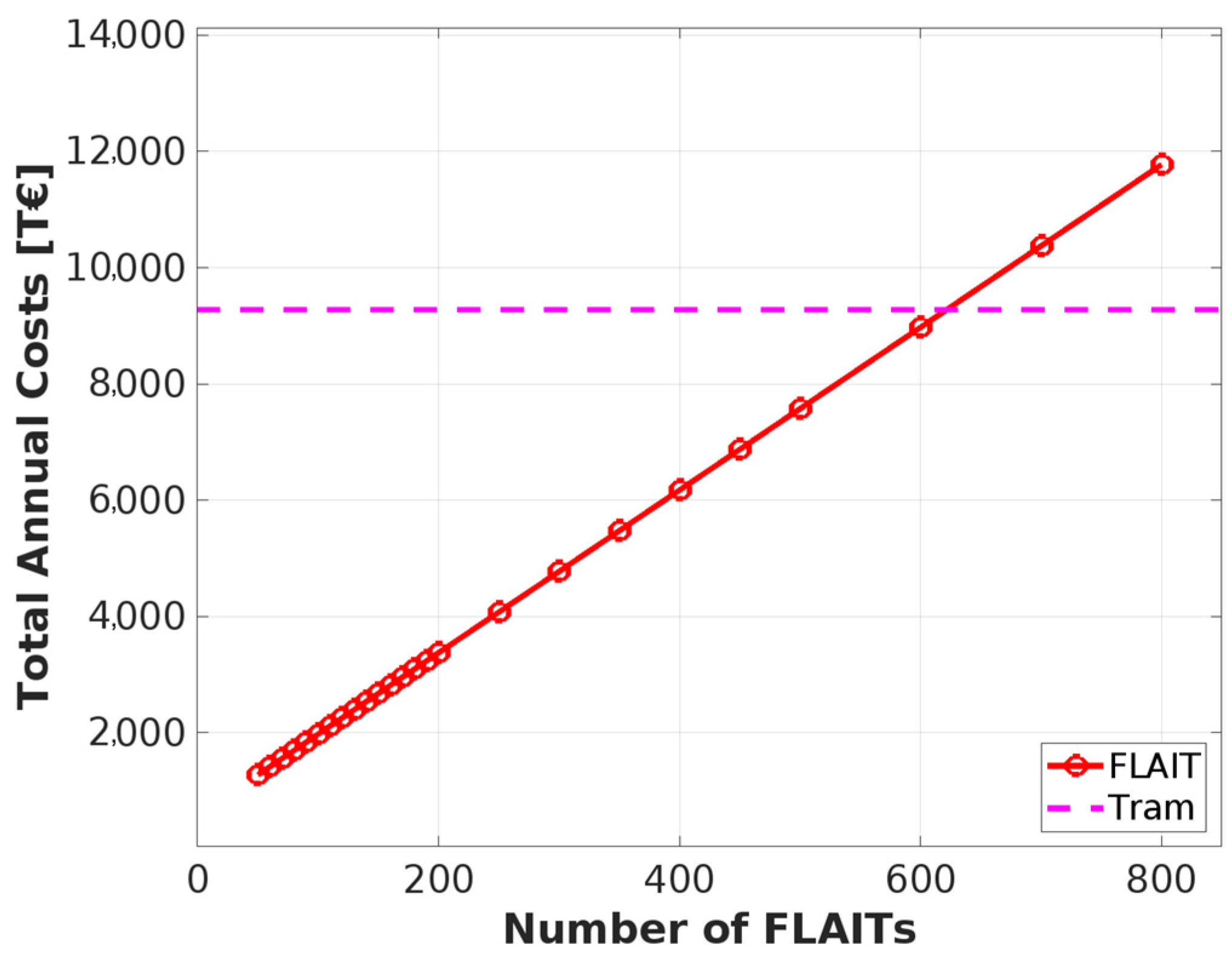
Some parameters have been taken from the literature to calculate the total annual costs of trams. According to [5], the investment costs for infrastructure amounted to 12 M€/km in 2008. The German inflation rates, published by the federal statistical office Germany in [58], have been considered to estimate the current costs. Furthermore, the lifetime of the relevant infrastructure has been taken from the official statement of the German Federal Ministry of Finance [59]. The vehicle cost of one tram, the operating cost per vehicle∙km and the annual mileage of the tram have been found in [5]. The lifetime of the tram has been stated in [48]. Using the Formula (9), including the parameters mentioned above, the annual costs of six trams, and the minimum tram number to cover the timetable of [51], amount to approximately 9,278 k€.
For the FLAIT-Trains, the investment costs for infrastructure and vehicles are in each case 1.8 M€/km and 37,500 € per vehicle without consideration of the volume discount. The annual operating costs amount to approximately 4,630 € per vehicle.
The simulation results of this key figure are shown in Figure 13. Due to the linear dependence of the vehicle numbers, the annual costs of FLAITs increased linearly with the increasing number of FLAITs. The annual costs of the service provider amounted to 1,276 k€ for 10 FLAITs, while the costs were 11,775 k€ for 800 FLAITs. From 700 FLAITs, the service provider must pay more costs (10,375 k€) for FLAITs than trams. In the future, the number of FLAITs with more costs than trams will not be considered.
6. Conclusions and Outlook
In this paper, an alternative system to the conventional tramway system has been simulatively investigated and analyzed. The pros and cons of tram and FLAIT-train are summarized in Table 4.
Five measures, the average waiting time per passenger, the maximum waiting time of a single passenger, the average travel time per passenger, the daily transportation productivity, and the total annual service provider’s costs, were considered in the system performance evaluation. An urban scenario based on the statistics was generated in the SUMO simulation environment. In this realistic scenario, it was shown from the simulation results that the transport capacity of the 30 tram trips according to the timetable in this scenario was covered by 170 FLAITs with better performances. The transport capacity comparison between trams and FLAIT trains is shown in Table 5.
In the simulations with FLAITs, the state of charge of the vehicle battery was not considered. Every FLAIT-train could drive without a battery charging. In future steps, the battery capacity, energy consumption, and the charging infrastructure (like a charging station) will be considered as the constraints in the simulations. Using that, the exact number of FLAIT-trains required in the realistic urban scenario can be determined.
Furthermore, the dispatching algorithm integrated into SUMO was used in this paper. According to the simulation results, only the average waiting time was considered as a cost function in the dispatching algorithm. There are some optimization potentials in the dispatching algorithm. If further key figures, like the maximum waiting time of a single passenger and total transport performance, are considered in the calculation of the cost function, a better transport capacity of the FLAIT-trains can be achieved.
The Krauss model with the perfect driver model was applied to modeling flexible platooning. Afterward, further available car-following models, e.g., the model for autonomous vehicles specified in [60], will be tried in further research.
As an intermediate solution of the FLAIT-Train, some problems of the conventional trams are still be solved by the considered FLAIT system, e.g., the large space occupancy. It could be improved in the next step to achieve fully autonomous FLAIT-Trains. Furthermore, one advantage of the FLAIT, no fixed stops, has not been considered in the simulations of this paper. It must be considered in future analysis.
Author Contributions
Conceptualization, S.W., T.W. and D.S.; methodology, S.W.; software, S.W.; validation, S.W., T.W. and D.S.; formal analysis, S.W.; resources, S.W.; data curation, S.W.; writing—original draft preparation, S.W.; writing—review and editing, S.W., T.W. and D.S.; visualization, S.W.; supervision, T.W. and D.S.; project administration, T.W. and D.S. All authors have read and agreed to the published version of the manuscript.
Funding
This research received no external funding.
Institutional Review Board Statement
Not applicable.
Informed Consent Statement
Not applicable.
Data Availability Statement
Restrictions apply to the availability of these data. Data were obtained from the DVG and are available from the authors with permission of the DVG.
Acknowledgments
We acknowledge support by the Open Access Publication Fund of the University of Duisburg-Essen.
Conflicts of Interest
The authors declare no conflict of interest.
References
- Bok, J.; Kwon, Y. Comparable Measures of Accessibility to Public Transport Using the General Transit Feed Specification. Sustainability 2016, 8, 224. [Google Scholar] [CrossRef] [Green Version]
- Murray, A.T.; Davis, R.; Stimson, R.J.; Ferreira, L. Public Transportation Access. Transp. Res. Part D Transp. Environ. 1998, 3, 319–328. [Google Scholar] [CrossRef] [Green Version]
- van Oort, N. Service Reliability and Urban Public Transport Design. Ph.D. Thesis, Delft University of Technology, Delft, The Netherlands, 2011. [Google Scholar]
- Suder, E.; Pfaffenbach, C. Alltagsmobilität in Kommunen zwischen Niederrhein und Ruhrgebiet. Aus welchen Gründen wird der ÖPNV nicht häufiger genutzt? Standort 2021, 45, 31–37. [Google Scholar] [CrossRef]
- Deutsch, V. Cost Pointers for the Implementation of Tramway and Bus Systems. Public Transp. Int. 2008, 57, 48–51. [Google Scholar]
- Parragh, S.N.; Doerner, K.F.; Hartl, R.F. A survey on pickup and delivery problems. J. Betr. 2008, 58, 81–117. [Google Scholar] [CrossRef]
- Ho, S.C.; Szeto, W.Y.; Kuo, Y.-H.; Leung, J.M.; Petering, M.; Tou, T.W. A survey of dial-a-ride problems: Literature review and recent developments. Transp. Res. Part B Methodol. 2018, 111, 395–421. [Google Scholar] [CrossRef]
- Cordeau, J.-F.; Laporte, G. The Dial-a-Ride Problem (DARP): Variants, modeling issues and algorithms. J. Belg. Fr. Ital. Oper. Res. Soc. 2003, 1, 89–101. [Google Scholar] [CrossRef]
- Drakoulis, R.; Bellotti, F.; Bakas, I.; Berta, R.; Paranthaman, P.K.; Dange, G.R.; Lytrivis, P.; Pagle, K.; de Gloria, A.; Amditis, A. A Gamified Flexible Transportation Service for On-Demand Public Transport. IEEE Trans. Intell. Transp. Syst. 2018, 19, 921–933. [Google Scholar] [CrossRef]
- McDonald, S.S. Personal Rapid Transit and Its Development. In Transportation Technologies for Sustainability; Springer: New York, NY, USA, 2013; pp. 831–850. [Google Scholar]
- Daszczuk, W.B. Measures of Structure and Operation of Automated Transit Networks. IEEE Trans. Intell. Transp. Syst. 2020, 21, 2966–2979. [Google Scholar] [CrossRef]
- Cordeau, J.-F.; Laporte, G. The dial-a-ride problem: Models and algorithms. Ann. Oper. Res. 2007, 153, 29–46. [Google Scholar] [CrossRef]
- Vansteenwegen, P.; Melis, L.; Aktaş, D.; Montenegro, B.D.G.; Vieira, F.S.; Sörensen, K. A survey on demand-responsive public bus systems. Transp. Res. Part C Emerg. Technol. 2022, 137, 103573. [Google Scholar] [CrossRef]
- Stein, D.M. Scheduling Dial-a-Ride Transportation Systems. Transp. Sci. 1978, 12, 232–249. [Google Scholar] [CrossRef]
- Psaraftis, H.N. A Dynamic Programming Solution to the Single Vehicle Many-to-Many Immediate Request Dial-a-Ride Problem. Transp. Sci. 1980, 14, 130–154. [Google Scholar] [CrossRef]
- Sexton, T.R.; Bodin, L.D. Optimizing Single Vehicle Many-to-Many Operations with Desired Delivery Times: I. Scheduling. Transp. Sci. 1985, 19, 378–410. [Google Scholar] [CrossRef]
- Sexton, T.R.; Bodin, L.D. Optimizing Single Vehicle Many-to-Many Operations with Desired Delivery Times: II. Routing. Transp. Sci. 1985, 19, 411–435. [Google Scholar] [CrossRef]
- Gupta, A.; Hajiaghayi, M.; Nagarajan, V.; Ravi, R. Dial a Ride from k-forest. ACM Trans. Algorithms 2010, 6, 1–21. [Google Scholar] [CrossRef]
- D’Souza, C.; Omkar, S.N.; Senthilnath, J. Pickup and delivery problem using metaheuristics techniques. Expert Syst. Appl. 2012, 39, 328–334. [Google Scholar] [CrossRef]
- Jaw, J.-J.; Odoni, A.R.; Psaraftis, H.N.; Wilson, N.H. A heuristic algorithm for the multi-vehicle advance request dial-a-ride problem with time windows. Transp. Res. Part B Methodol. 1986, 20, 243–257. [Google Scholar] [CrossRef]
- Cordeau, J.-F.; Laporte, G. A tabu search heuristic for the static multi-vehicle dial-a-ride problem. Transp. Res. Part B Methodol. 2003, 37, 579–594. [Google Scholar] [CrossRef] [Green Version]
- Jorgensen, R.M.; Larsen, J.; Bergvinsdottir, K.B. Solving the Dial-a-Ride problem using genetic algorithms. J. Oper. Res. Soc. 2007, 58, 1321–1331. [Google Scholar] [CrossRef]
- Parragh, S.N.; Schmid, V. Hybrid column generation and large neighborhood search for the dial-a-ride problem. Comput. Oper. Res. 2013, 40, 490–497. [Google Scholar] [CrossRef] [PubMed]
- Melis, L.; Sörensen, K. The real-time on-demand bus routing problem: What is the cost of dynamic requests. Comput. Oper. Res. 2022, 147, 105941. [Google Scholar] [CrossRef]
- Desrosiers, J.; Dumas, Y.; Soumis, F.; Taillefer, S.; Villeneuve, D. An Algorithm for Mini-Clustering in Handicapped Transport; Cahiers du GERAD: Montréal, QC, Canada, 1991. [Google Scholar]
- Ioachim, I.; Desrosiers, J.; Dumas, Y.; Solomon, M.M.; Villeneuve, D. A Request Clustering Algorithm for Door-to-Door Handicapped Transportation. Transp. Sci. 1995, 29, 63–78. [Google Scholar] [CrossRef]
- Rekiek, B.; Delchambre, A.; Saleh, H.A. Handicapped Person Transportation: An application of the Grouping Genetic Algorithm. Eng. Appl. Artif. Intell. 2006, 19, 511–520. [Google Scholar] [CrossRef]
- Atahran, A.; Lenté, C.; T’kindt, V. A Multicriteria Dial-a-Ride Problem with an Ecological Measure and Heterogeneous Vehicles. J. Multi-Crit. Decis. Anal. 2014, 21, 279–298. [Google Scholar] [CrossRef]
- Garaix, T.; Artigues, C.; Feillet, D.; Josselin, D. Optimization of occupancy rate in dial-a-ride problems via linear fractional column generation. Comput. Oper. Res. 2011, 38, 1435–1442. [Google Scholar] [CrossRef] [Green Version]
- Parragh, S.N.; Pinho de Sousa, J.; Almada-Lobo, B. The Dial-a-Ride Problem with Split Requests and Profits. Transp. Sci. 2015, 49, 311–334. [Google Scholar] [CrossRef] [Green Version]
- Borndörfer, R.; Grötschel, M.; Klostermeier, F.; Küttner, C. Telebus Berlin: Vehicle Scheduling in a Dial-a-Ride System. In Computer-Aided Transit Scheduling; Springer: Berlin/Heidelberg, Germany, 1999; pp. 391–422. ISBN 9783642859700. [Google Scholar]
- Rigas, E.S.; Ramchurn, S.D.; Bassiliades, N. Algorithms for electric vehicle scheduling in large-scale mobility-on-demand schemes. Artif. Intell. 2018, 262, 248–278. [Google Scholar] [CrossRef] [Green Version]
- Lim, A.; Zhang, Z.; Qin, H. Pickup and Delivery Service with Manpower Planning in Hong Kong Public Hospitals. Transp. Sci. 2017, 51, 688–705. [Google Scholar] [CrossRef]
- Pimenta, V.; Quillot, A.; Toussaint, H.; Vigo, D. Models and algorithms for reliability-oriented dial-a-ride with autonomous electric vehicles. Eur. J. Oper. Res. 2017, 257, 601–613. [Google Scholar] [CrossRef]
- Zwick, F.; Axhausen, K.W. Ride-pooling demand prediction: A spatiotemporal assessment in Germany. J. Transp. Geogr. 2022, 100, 103307. [Google Scholar] [CrossRef]
- Knie, A.; Ruhrort, L.; Gödde, J.; Pfaff, T. Ride-Pooling-Dienste und Ihre Bedeutung für den Verkehr. Nachfragemuster und Nutzungsmotive am Beispiel von “CleverShuttle”—Eine Untersuchung auf Grundlage von Buchungsdaten und Kundenbefragungen in vier Deutschen Städten; WZB Discussion Paper SP III 2020-601. 2020. Available online: https://www.econstor.eu/handle/10419/220020 (accessed on 29 December 2022).
- Viergutz, K.K.; Brinkmann, F. Ride-pooling—A model for success? Digitisation in local public transport. SIGNAL + DRAHT 2018, 7 + 8, 13–18. [Google Scholar]
- Gebhardt, L.; Brost, M.; Steiner, T. Bus on demand—Ein Mobilitätskonzept mit Zukunft: Das Reallabor Schorndorf zieht nach dem Testbetrieb Bilanz. GAIA—Ecol. Perspect. Sci. Soc. 2019, 28, 70–72. [Google Scholar] [CrossRef]
- Fischer, H. FLAIT—Netzwerkgestütztes Mobilitätssystem zum autonomen Betrieb von Fahrzeugflotten. In Mobilität in Zeiten der Veränderung; Proff, H., Ed.; Springer Fachmedien Wiesbaden: Wiesbaden, Germany, 2019; pp. 211–227. ISBN 9783658261061. [Google Scholar]
- Infas Institut für Angewandte Sozialwissenschaft. Mobilität in Deutschland 2017—Tabellenband, Bonn. 2018. Available online: http://www.mobilitaet-in-deutschland.de/pdf/MiD2017_Tabellenband_Deutschland.pdf (accessed on 28 March 2022).
- Netzsieger. “Durchschnittsgeschwindigkeit der Stadtbahnen in ausgewählten deutschen Städten (in Kilometer pro Stunde; Stand: 2016).” Chart. 19 April 2018. Statista. Available online: https://de.statista.com/statistik/daten/studie/921422/umfrage/durchschnittsgeschwindigkeit-der-stadtbahnen-in-deutschland/ (accessed on 24 November 2022).
- INRIX. “Durchschnittliche Geschwindigkeit im Autoverkehr in ausgewählten deutschen Städten im Jahr 2018 (in Meilen pro Stunde).” Chart. 12 February 2019. Statista. Available online: https://de.statista.com/statistik/daten/studie/994676/umfrage/innerstaedtische-durchschnittsgeschwindigkeit-im-autoverkehr-in-deutschen-staedten/ (accessed on 24 November 2022).
- Varrier, E. Urbanloop: Retour vers le Futur. Les Tablettes Lorraines 2019, 1917, 20. [Google Scholar]
- Vuchic, V.R. Urban Transit Systems and Technology; John Wiley & Sons: Hoboken, NJ, USA, 2007; ISBN 0470168064. [Google Scholar]
- Alonso-Mora, J.; Samaranayake, S.; Wallar, A.; Frazzoli, E.; Rus, D. On-demand high-capacity ride-sharing via dynamic trip-vehicle assignment. Proc. Natl. Acad. Sci. USA 2017, 114, 462–467. [Google Scholar] [CrossRef] [Green Version]
- Babicheva, T.; Burghout, W.; Andreasson, I.; Faul, N. The matching problem of empty vehicle redistribution in autonomous taxi systems. Procedia Comput. Sci. 2018, 130, 119–125. [Google Scholar] [CrossRef]
- Klatt, S. Die Ökonomische Bedeutung der Qualität von Verkehrsleistungen; Duncker & Humblot: Berlin, Germany, 1965; ISBN 9783428407781. [Google Scholar]
- Hass-Klau, C.; Crampton, G.; Biereth, C.; Deutsch, V. Bus or Light Rail: Making the Right Choice.: A Financial, Operational, and Demand Comparison of Light Rail, Guided Buses, Busways, and Bus Lanes, 2nd ed.; Government of the United Kingdom—Environmental and Transport Planning: Brighton, UK, 2003; ISBN 0951962086.
- Stadt Duisburg. Zahlen, Daten, Fakten. Available online: https://www.duisburg.de/wohnenleben/zahlen_daten_fakten/zahlen-daten-fakten.php (accessed on 30 March 2022).
- Stadt Mülheim an der Ruhr. Bevölkerungsbestand. Available online: https://www.muelheim-ruhr.de/cms/bevoelkerungsbestand1.html (accessed on 30 March 2022).
- DVG. Fahrplan 901. 2021. Available online: https://www.dvg-duisburg.de/fileadmin/Media/Downloads/Linienplaene/Bahn/DVG_Fahrplan_901.pdf (accessed on 20 September 2022).
- File:Dvg1029wis220605.jpg—Wikimedia Commons. Available online: https://commons.wikimedia.org/wiki/File:Dvg1029wis220605.jpg (accessed on 23 March 2022).
- Ma, X. Effects of Vehicles with Different Degrees of Automation on Traffic Flow in Urban Areas. Ph.D. Thesis, University of Duisburg-Essen, Duisburg, Germany, 2021. [Google Scholar]
- Weber, T. On the Potential of a Weather-Related Road Surface Condition Sensor Using an Adaptive Generic Framework in the Context of Future Vehicle Technology. Ph.D. Thesis, University of Duisburg-Essen, Duisburg, Germany, 2022. [Google Scholar]
- Persons—SUMO Documentation. Available online: https://sumo.dlr.de/docs/Specification/Persons.html (accessed on 10 December 2022).
- Schmidt, G.; Thomas, B. Hochrechnungsfaktoren für Manuelle und Automatische Kurzzeitzählungen im Innerortsbereich; Bundesministerium für Verkehr: Bonn, Germany, 1996. [Google Scholar]
- Segata, M. Safe and Efficient Communication Protocols for Platooning Control. Ph.D. Thesis, University of Trento, Trento, Italy, University of Innsbruck, Innsbruck, Austria, 2016. [Google Scholar]
- Krauss, S. Microscopic Modeling of Traffic Flow: Investigation of Collision Free Vehicle Dynamics. Ph.D. Thesis, DLR, Abt. Unternehmensorganisation und—Information, Cologne, Germany, 1998. [Google Scholar]
- German Federal Ministry of Finance. AfA-Tabelle für den Wirtschaftszweig “Personen- und Güterbeförderung (im Straßen- und Schienenverkehr)”. Available online: https://www.bundesfinanzministerium.de/Content/DE/Standardartikel/Themen/Steuern/Weitere_Steuerthemen/Betriebspruefung/AfA-Tabellen/AfA-Tabelle_Personen-und-Gueterbefoerderung.html (accessed on 4 September 2022).
- Milanés, V.; Shladover, S.E. Modeling cooperative and autonomous adaptive cruise control dynamic responses using experimental data. Transp. Res. Part C Emerg. Technol. 2014, 48, 285–300. [Google Scholar] [CrossRef]
Figure 1.
FLAIT Vehicle.

Figure 2.
Sensors of a FLAIT.

Figure 3.
System of FLAIT Trains.

Figure 4.
Flow Chart of Methodology.

Figure 5.
Tram Route of Line 901 between Duisburg Central Station and Mülheim Central Station.

Figure 6.
DVG DC-10 NC-DU [52].
Figure 6.
DVG DC-10 NC-DU [52].

Figure 7.
Distribution of Counted Boarding Passengers: (a) According to the Tram Stops; (b) According to the Hours.
Figure 7.
Distribution of Counted Boarding Passengers: (a) According to the Tram Stops; (b) According to the Hours.

Figure 13.
Total Annual Costs.


Table 1.
A Comparison between Four Public Transportation Services based on [7].
Table 1.
A Comparison between Four Public Transportation Services based on [7].
| Tram | Known On-Demand Transit | Taxi | FLAIT-Train | PRT | |
|---|---|---|---|---|---|
| Route | fixed | flexible | flexible | fixed | fixed |
| Stop | fixed | w/o | w/o | w/o | fixed |
| Schedule | fixed | by request | by request | by request | by request |
| Ticket Cost | low | medium | high | low | low |
| Mode | shared | shared | non-shared | shared 1 | shared 1 |
| Seating Capacity | >100 | <50 | <7 | 2 | 2–4 |
| Autonomous Level | no | no | no | automated | fully |
| Track Usage | exclusive | mixed | mixed | exclusive | exclusive |
| Reservation | not needed | often needed | not needed | not needed 2 | not needed |
| Avg. Speed [kph] | 33.5 3 | 23 4 | 23 4 | 32 | 60 5 |
Table 2.
Vehicle Parameters.
| DVG GT-10 NC-DU | FLAIT | |
|---|---|---|
| Passenger Capacity | 176 | 2 |
| Maximum Speed | 70 kph | 80 kph |
| Normal Acceleration | 1.3 m/s2 | 2.5 m/s2 |
| Normal Deceleration | −1.1 m/s2 | −2.5 m/s2 |
Table 3.
Hourly Passenger Distribution derived according to [56] and according to Statistics.
Table 3.
Hourly Passenger Distribution derived according to [56] and according to Statistics.
| Name | Hourly Percentage Passenger Distribution [%] | ||||||||||||||||||||
|---|---|---|---|---|---|---|---|---|---|---|---|---|---|---|---|---|---|---|---|---|---|
| 3 | 4 | 5 | 6 | 7 | 8 | 9 | 10 | 11 | 12 | 13 | 14 | 15 | 16 | 17 | 18 | 19 | 20 | 21 | 22 | 23 | |
| TGw2_PKW [57] | 0.3 | 0.4 | 1.2 | 4.6 | 7.5 | 6.7 | 5.3 | 5.1 | 5.1 | 5.3 | 5.4 | 5.7 | 6.8 | 8.5 | 8.7 | 7.5 | 5.1 | 4.0 | 3.1 | 2.1 | 1.6 |
| DU-MUE | 0.0 | 0.7 | 1.5 | 3.0 | 11.1 | 7.4 | 5.6 | 4.9 | 5.0 | 6.0 | 8.4 | 7.7 | 8.2 | 9.6 | 7.5 | 5.4 | 3.6 | 2.1 | 1.0 | 0.9 | 0.4 |
Table 4.
Pros & Cons of Trams and FLAIT-Trains.
| Tram | FLAIT-Train | |
|---|---|---|
| Pros |
|
|
| Cons |
|
|
Table 5.
Transport Capacity Comparison between Trams and 170 FLAIT-Train.
| Time Period | Tram | 170 FLAIT-Train | |
|---|---|---|---|
| Passenger Capacity per Vehicle | - | 176 | 2 |
| Average Waiting Time [min] | Mornings | 6.7 | 4.7 |
| Afternoons | 7.0 | 3.9 | |
| Whole Day | 6.9 | 4.2 | |
| Maximum Waiting Time [min] | Mornings | 18 | 28.9 |
| Afternoons | 30 | 26.5 | |
| Whole Day | 30 | 28.9 | |
| Average In-Vehicle Time [min] | Mornings | 7.7 | 5.2 |
| Afternoons | 6.9 | 4.7 | |
| Whole Day | 7.2 | 4.9 | |
| Daily Transportation Productivity [Persons∙km/day] | Mornings | 511,146 | 724,937 |
| Afternoons | 555,478 | 796,563 | |
| Whole Day | 537,181 | 767,002 | |
| Total Annual Costs [k€] | - | 9,278 | 2,956 |
| Operator’s Annual Operating Costs [€/km] | - | 66.9 1 | 39.3 |
1 Determined according to [5] taking the German inflation rates into account.
Disclaimer/Publisher’s Note: The statements, opinions and data contained in all publications are solely those of the individual author(s) and contributor(s) and not of MDPI and/or the editor(s). MDPI and/or the editor(s) disclaim responsibility for any injury to people or property resulting from any ideas, methods, instructions or products referred to in the content. |
© 2022 by the authors. Licensee MDPI, Basel, Switzerland. This article is an open access article distributed under the terms and conditions of the Creative Commons Attribution (CC BY) license (https://creativecommons.org/licenses/by/4.0/).
Share and Cite
MDPI and ACS Style
Wang, S.; Weber, T.; Schramm, D. Simulative Study of an Innovative On-Demand Transport System Using a Realistic German Urban Scenario. Future Transp. 2023, 3, 38-56. https://doi.org/10.3390/futuretransp3010003
AMA Style
Wang S, Weber T, Schramm D. Simulative Study of an Innovative On-Demand Transport System Using a Realistic German Urban Scenario. Future Transportation. 2023; 3(1):38-56. https://doi.org/10.3390/futuretransp3010003
Chicago/Turabian StyleWang, Shen, Thomas Weber, and Dieter Schramm. 2023. "Simulative Study of an Innovative On-Demand Transport System Using a Realistic German Urban Scenario" Future Transportation 3, no. 1: 38-56. https://doi.org/10.3390/futuretransp3010003