Development of a Turning Movement Estimator Using CV Data


Abstract
:1. Introduction
2. Material and Methods
2.1. Literature Review
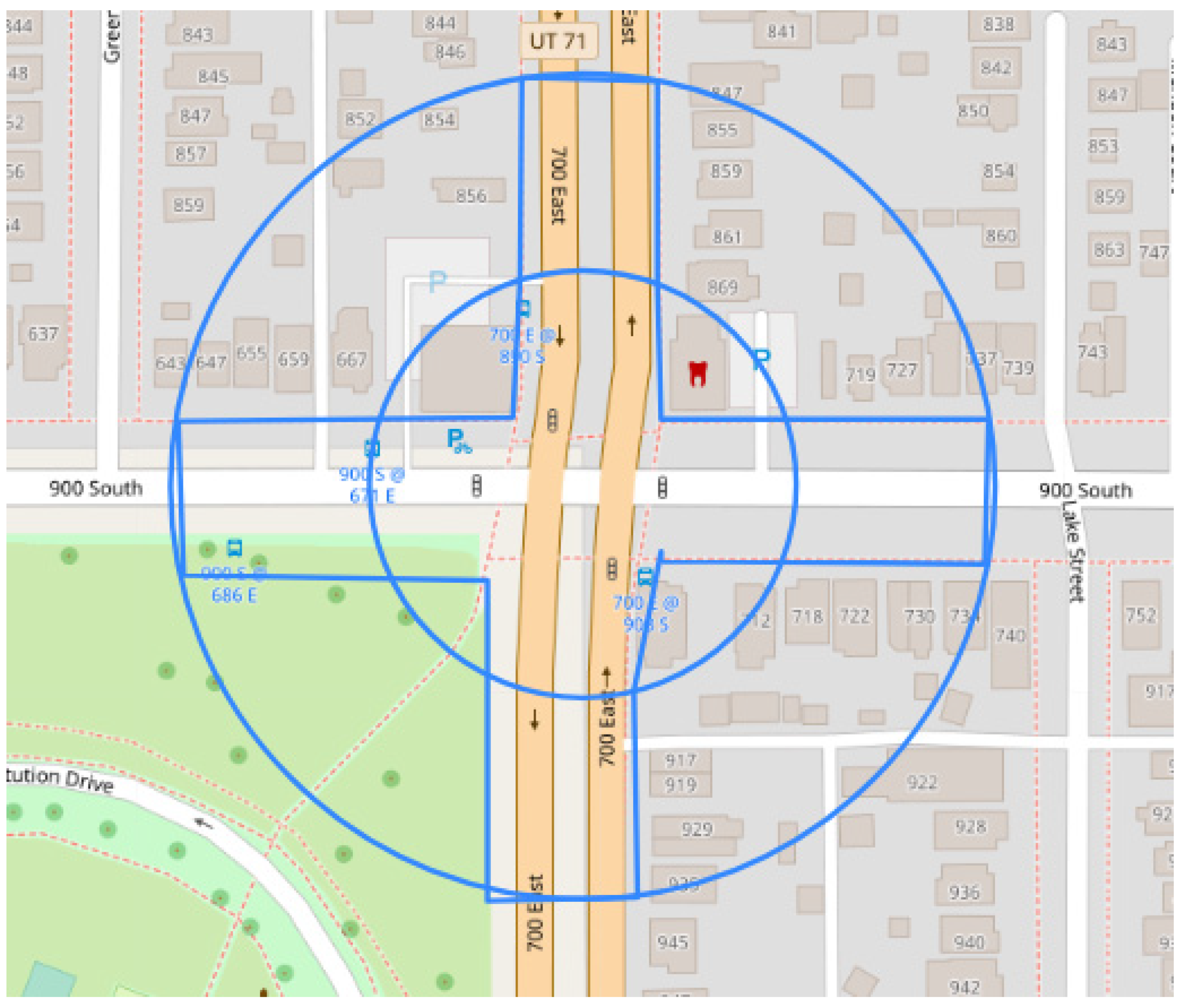
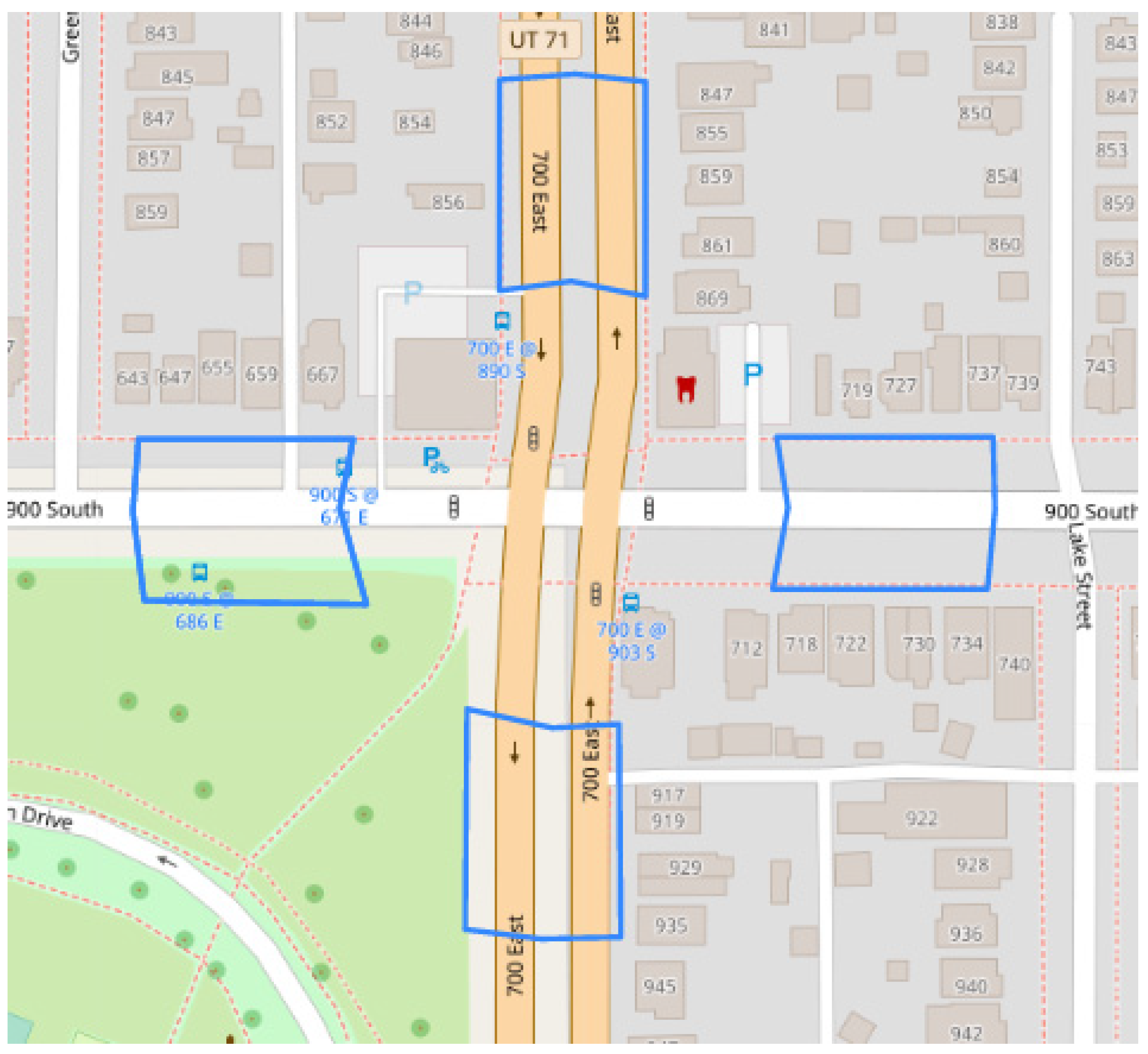
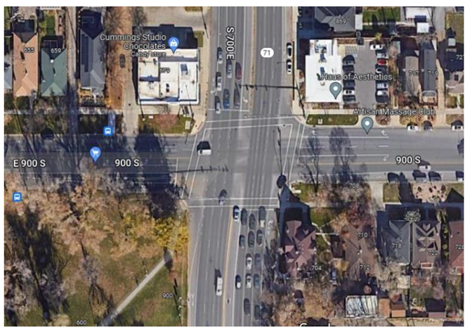
2.2. Data Collection
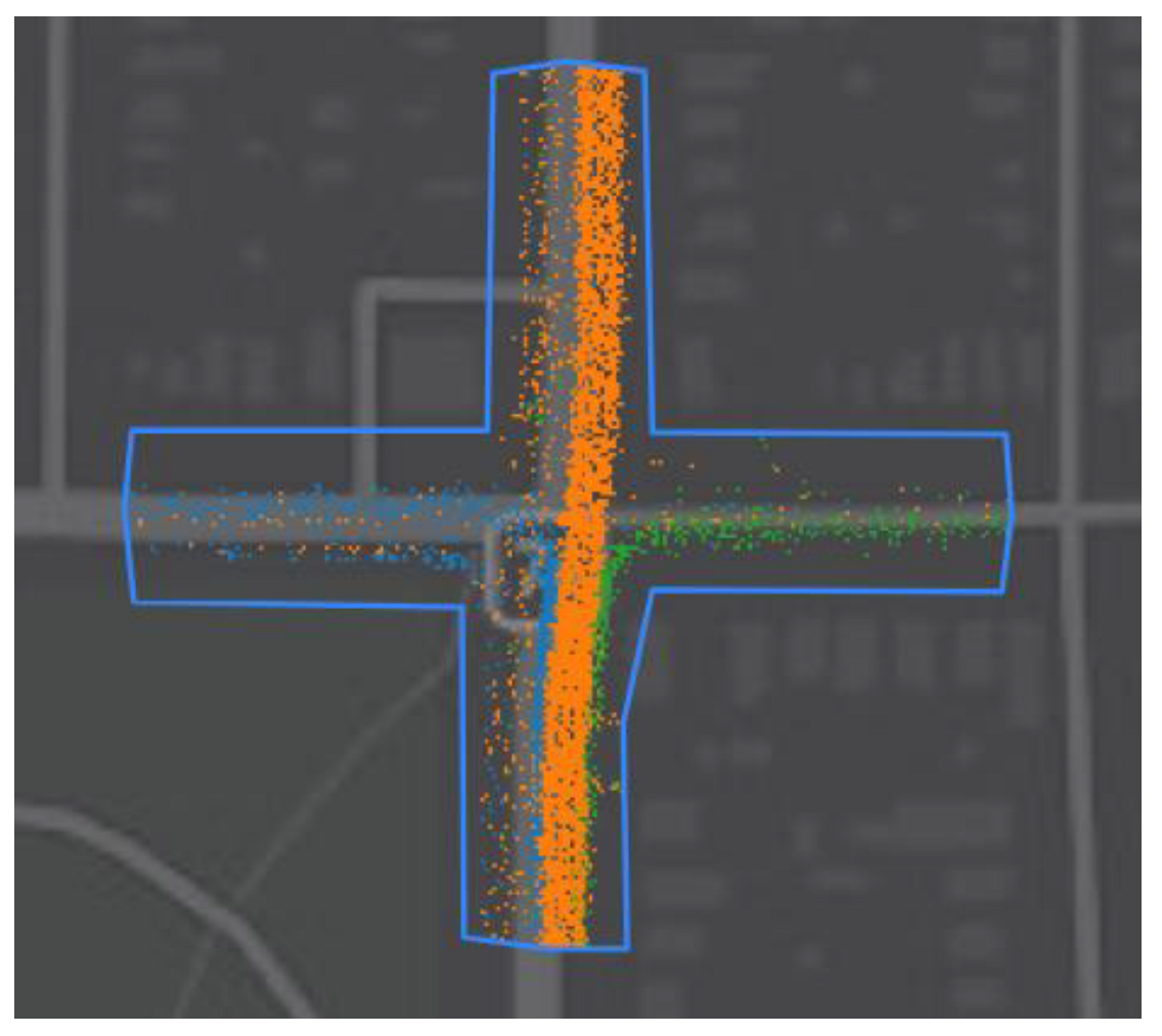
2.3. Data Processing
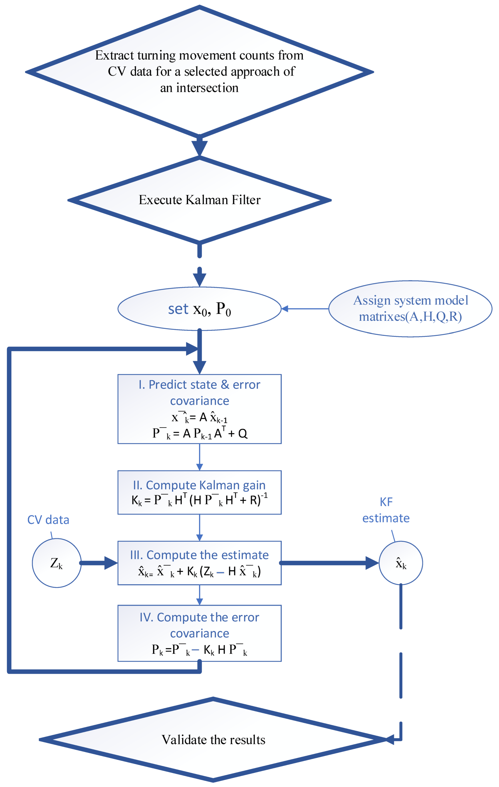
2.4. Methodology
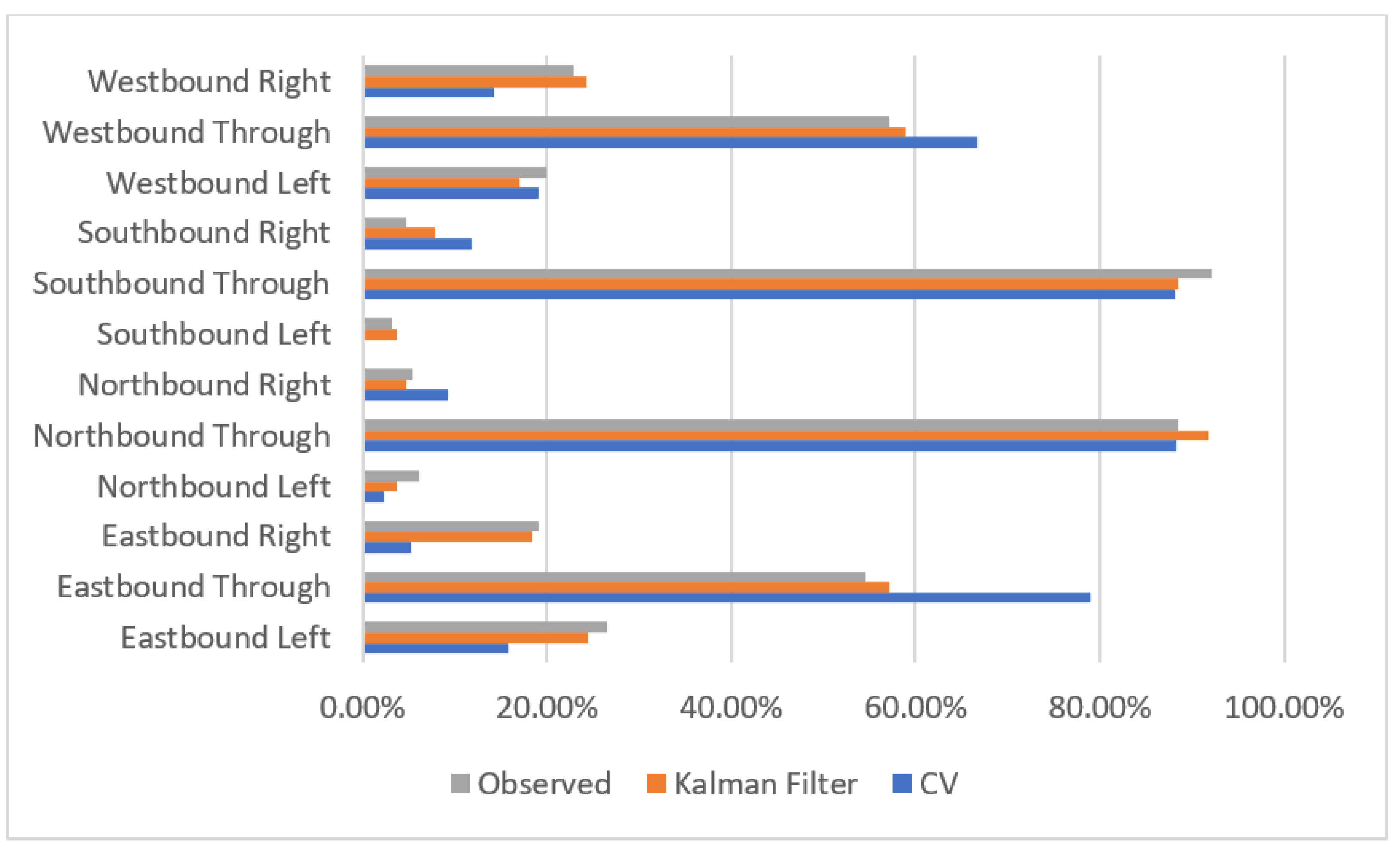
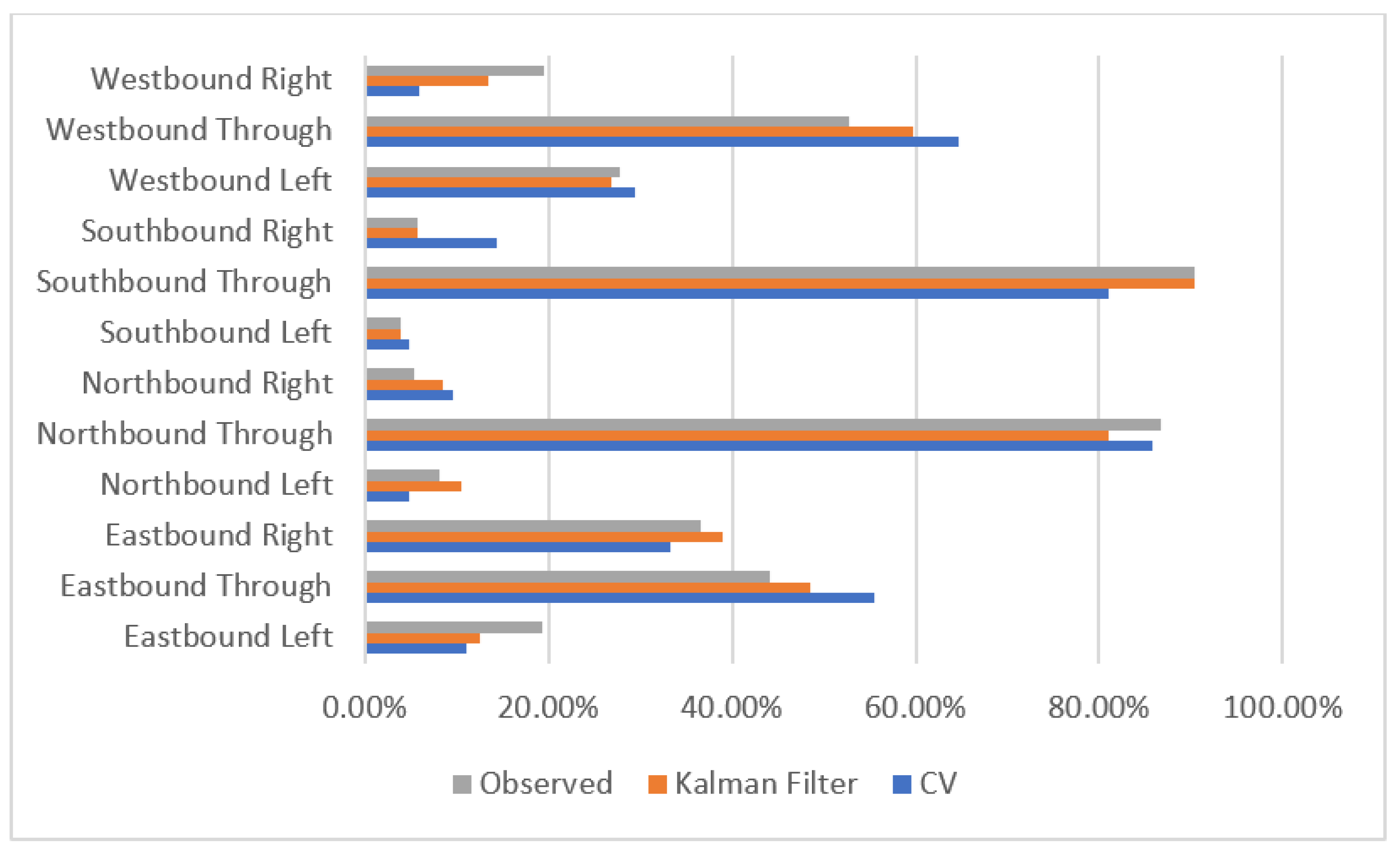
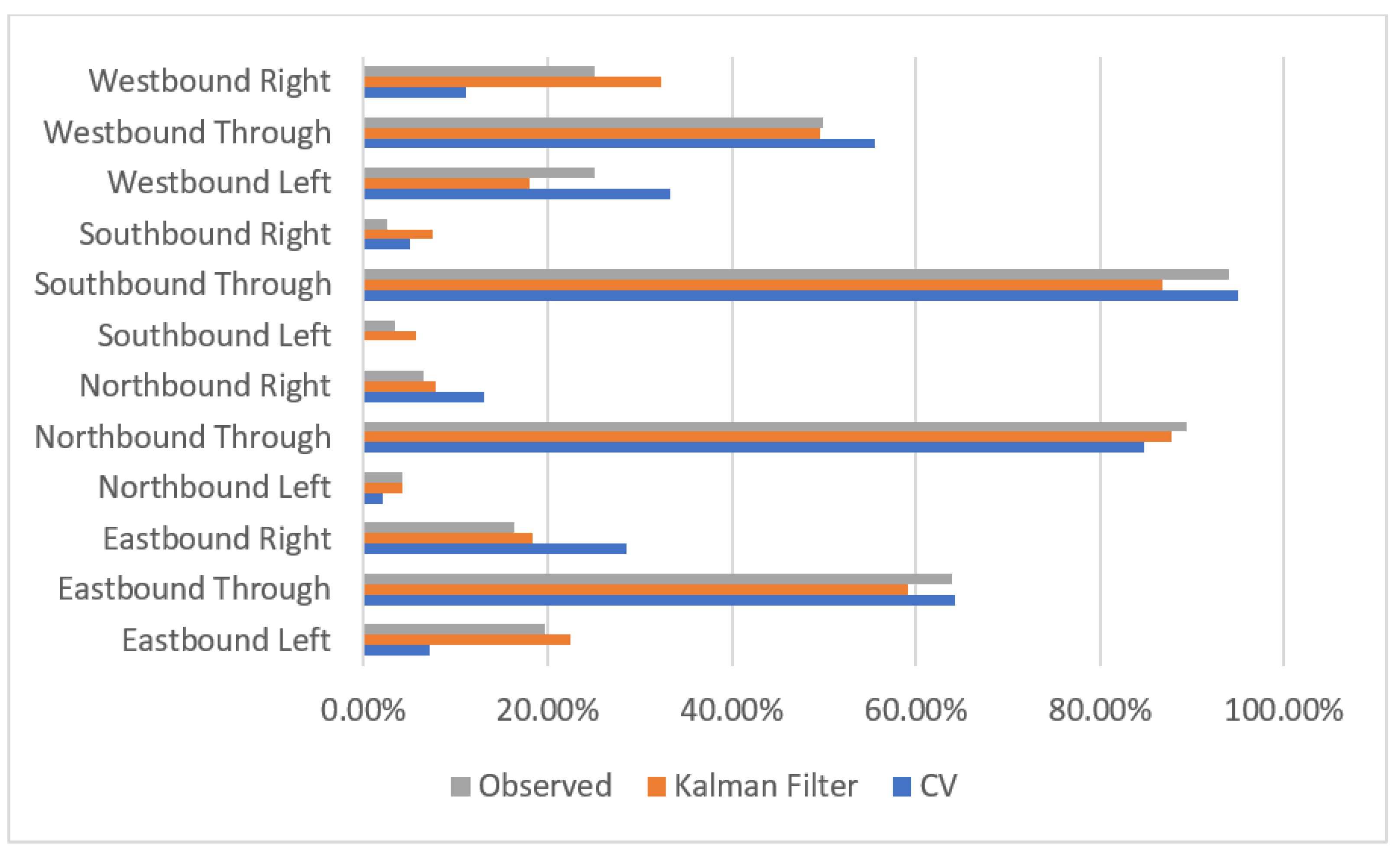
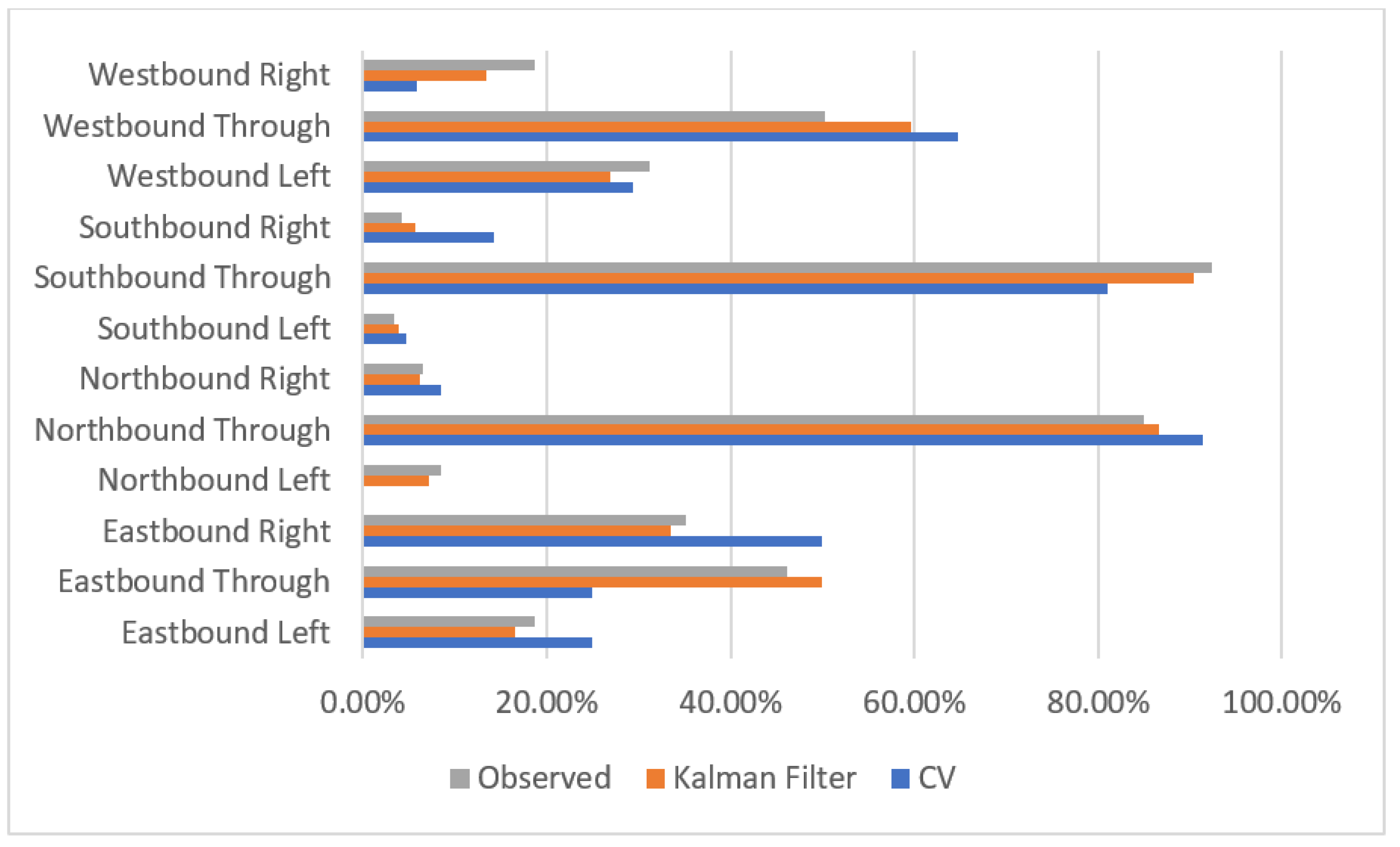
3. Results
4. Discussion
Author Contributions
Funding
Informed Consent Statement
Data Availability Statement
Acknowledgments
Conflicts of Interest
References
- Noyce, D.A.; Bill, A.R.; Chitturi, M.v.; Santiago-Chaparro, K.R. Turning Movement Counts on Shared Lanes: Prototype Development and Analysis Procedures Final Report for NCHRP IDEA Project 198. 2019. Available online: https://trid.trb.org/view/1652249 (accessed on 15 June 2022).
- Xu, K.; Yi, P.; Shao, C.; Mao, J. Development and Testing of an Automatic Turning Movement Identification System at Signalized Intersections. J. Transp. Technol. 2013, 3, 241–246. [Google Scholar] [CrossRef] [Green Version]
- Hauer, E.; Pagitsas, E.; Shin, B.T. Estimation of Turning Flows from Automatic Counts. Transp. Res. Rec. 1981, 795, 1–7. [Google Scholar]
- Vigos, G.; Papageorgiou, M. A Simplified Estimation Scheme for the Number of Vehicles in Signalized Links. IEEE Trans. Intell. Transp. Syst. 2010, 11, 312–321. [Google Scholar] [CrossRef]
- Karapetrovic, J.; Martin, P.T. Estimation of Intersection Turning Movement Flows with the TMERT3 Model Version: Sensitivity to a Widespread Detector Failure. Int. J. Traffic Transp. Eng. 2021, 11, 442–453. [Google Scholar] [CrossRef]
- Qi, H.; Dai, R.; Tang, Q.; Hu, X. Quasi-Real Time Estimation of Turning Movement Spillover Events Based on Partial Connected Vehicle Data. Transp. Res. Part C Emerg. Technol. 2020, 120, 102824. [Google Scholar] [CrossRef]
- Nihan, N.L.; Davis, G.A. Application of Prediction-Error Minimization and Maximum Likelihood to Estimate Intersection O-D Matrices from Traffic Counts. Transp. Sci. 1989, 23, 77–90. [Google Scholar] [CrossRef]
- Maher, M.J. Estimating the Turning Flows at a Junction: A Comparison of Three Models. Transp. Res. Board 1984, 25, 19–22. [Google Scholar]
- Mahmoud, N.; Abdel-Aty, M.; Cai, Q.; Yuan, J. Predicting Cycle-Level Traffic Movements at Signalized Intersections Using Machine Learning Models. Transp. Res. Part C Emerg. Technol. 2021, 124, 102930. [Google Scholar] [CrossRef]
- Virkler, M.R.; Kumar, N.R. System to Identify Turning Movements at Signalized Intersections. J. Transp. Eng. 1998, 124, 607–609. [Google Scholar] [CrossRef]
- Noyce, D.; Chittori, M.; Santiago-Chaparro, K.; Bill, A.R. Automated Turning Movement Counts for Shared Lanes Using Existing Vehicle Detection Infrastructure Final Report for NCHRP IDEA Project 177. 2016. Available online: https://trid.trb.org/view/1422700 (accessed on 15 June 2022).
- Shirazi, M.S.; Morris, B. Vision-Based Turning Movement Counting at Intersections by Cooperating Zone and Trajectory Comparison Modules. In Proceedings of the 2014 17th IEEE International Conference on Intelligent Transportation Systems, ITSC 2014, Qingdao, China, 8–11 October 2014; Institute of Electrical and Electronics Engineers Inc.: Piscataway, NJ, USA, 2014; pp. 3100–3105. [Google Scholar] [CrossRef] [Green Version]
- Yi, P.; Zhang, S. Development and Field Testing of an Automatic Turning Movement Identification System; State Job Number: 135141; The Ohio Department of Transportation, Office of Statewide Planning & Research: Columbus, OH, USA, 2017. [Google Scholar]
- Shirazi, M.S.; Morris, B.T. Vision-Based Turning Movement Monitoring: Count, Speed & Waiting Time Estimation. IEEE Intell. Transp. Syst. Mag. 2016, 8, 23–34. [Google Scholar] [CrossRef]
- Bélisle, F.; Saunier, N.; Bilodeau, G.A.; le Digabel, S. Optimized Video Tracking for Automated Vehicle Turning Movement Counts. Transp. Res. Rec. 2017, 2645, 104–112. [Google Scholar] [CrossRef]
- Santiago-Chaparro, K.R.; Chitturi, M.; Bill, A.; Noyce, D.A. Automated Turning Movement Counts for Shared Lanes: Leveraging Vehicle Detection Data. Transp. Res. Rec. 2016, 2558, 30–40. [Google Scholar] [CrossRef]
- Ghanim, M.S.; Shaaban, K. Estimating Turning Movements at Signalized Intersections Using Artificial Neural Networks. IEEE Trans. Intell. Transp. Syst. 2019, 20, 1828–1836. [Google Scholar] [CrossRef]
- Shaaban, K.; Hamdi, A.; Ghanim, M.; Shaban, K.B. Machine Learning-Based Multi-Target Regression to Effectively Predict Turning Movements at Signalized Intersections. Int. J. Transp. Sci. Technol. 2022, 12, 245–257. [Google Scholar] [CrossRef]
- Mechler, A.M.; Machemehl, R.B.; Lee, C.E.; Rpo, G. The Design of an Automated Traffic Counting System with Turning Movement; Center for Transportation Research, The University of Texas at Austin: Austin, TX, USA, 1986. [Google Scholar]
- Gholami, A.; Tian, Z. Using Stop Bar Detector Information to Determine Turning Movement Proportions in Shared Lanes. J. Adv. Transp. 2016, 50, 802–817. [Google Scholar] [CrossRef] [Green Version]
- Ghods, A.H.; Fu, L. Real-Time Estimation of Turning Movement Counts at Signalized Intersections Using Signal Phase Information. Transp. Res. Part C Emerg. Technol. 2014, 47, 128–138. [Google Scholar] [CrossRef]
- Karapetrovic, J.; Martin, P.T. Estimating Intersection Turning Movement Flows with a NETFLO Algorithm: Weight Constraint Calibration. Adv. Transp. Stud. 2020, 52, 73–88. [Google Scholar] [CrossRef]
- Zheng, J.; Liu, H.X. Estimating Traffic Volumes for Signalized Intersections Using Connected Vehicle Data. Transp. Res. Part C Emerg. Technol. 2017, 79, 347–362. [Google Scholar] [CrossRef] [Green Version]
- Tang, K.; Tan, C.; Cao, Y.; Yao, J.; Sun, J. A Tensor Decomposition Method for Cycle-Based Traffic Volume Estimation Using Sampled Vehicle Trajectories. Transp. Res. Part C Emerg. Technol. 2020, 118, 102739. [Google Scholar] [CrossRef]
- Carranza, S. Scalable Operational Traffic Signal Performance Measures from Vehicle Trajectory Data; Purdue University: West Lafayette, IN, USA, 2021. [Google Scholar]
- Saldivar-Carranza, E.D.; Li, H.; Bullock, D.M. Identifying Vehicle Turning Movements at Intersections from Trajectory Data. In Proceedings of the 2021 IEEE International Intelligent Transportation Systems Conference (ITSC), Indianapolis, IN, USA, 19–22 September 2021; Institute of Electrical and Electronics Engineers Inc.: Piscataway, NJ, USA, 2021; Volume 2021, pp. 4043–4050. [Google Scholar] [CrossRef]
- Available online: http://www.wejo.com (accessed on 18 July 2022).
- National Research Council (U.S.); Transportation Research Board. Highway Capacity Manual; Transportation Research Board, National Research Council: Washington, DC, USA, 2000. [Google Scholar]
- Kalman, R.E. A New Approach to Linear Filtering and Prediction Problems. J. Basic Eng. 1960, 82, 35–45. [Google Scholar] [CrossRef] [Green Version]
- van Lint, H.; Djukic, T. Applications of Kalman Filtering in Traffic Management and Control. In 2012 TutORials in Operations Research; INFORMS: Catonsville, MD, USA, 2012; pp. 59–91. [Google Scholar] [CrossRef] [Green Version]
- Kim, P. Kalman Filter for Beginners: With MATLAB Examples; A-JIN Publishing Company: Seoul, Republic of Korea, 2011. [Google Scholar]
- Bishop, G.; Welch, G. An Introduction to the Kalman Filter; SIGGRAPH ACM, Inc.: Los Angeles, CA, USA, 2001. [Google Scholar]
- Hunter, M.; Mathew, J.K.; Li, H.; Bullock, D.M. Estimation of Connected Vehicle Penetration on US Roads in Indiana, Ohio, and Pennsylvania. J. Transp. Technol. 2021, 11, 597–610. [Google Scholar] [CrossRef]


| External Input | (Measurement) |
|---|---|
| Final output | (estimate) |
| System model | |
| For internal computation | , , , |
| Metric | KF vs. Ground Truth % | CV vs. Ground Truth % |
|---|---|---|
| Number of Cases | 48 | 48 |
| Mean | 2.15 | 5.89 |
| Standard Deviation | 2.23 | 5.93 |
| Min | 0.10 | 0.15 |
| 25% Quantile | 0.38 | 1.05 |
| 50% Quantile | 1.60 | 3.80 |
| 75% Quantile | 3.05 | 9.65 |
| Max | 9.40 | 24.50 |
| RMSE | 3.07 | 8.31 |
| Metric | KF vs. Ground Truth % | CV vs. Ground Truth % |
|---|---|---|
| Number of Cases | 7 | 7 |
| Mean | 3.91 | 0.97 |
| Standard Deviation | 2.11 | 8.44 |
| Min | 0.30 | 0.15 |
| 25% Quantile | 3.10 | 0.28 |
| 50% Quantile | 4.30 | 0.90 |
| 75% Quantile | 4.70 | 1.40 |
| Max | 7.20 | 2.40 |
| Source of Data | Min Residual % | Max Residual % | RMSE % |
|---|---|---|---|
| Two months | 0.04 | 7.00 | 3.06 |
| One month | 0.1 | 9.40 | 3.07 |
| Metric | KF vs. Ground Truth % | CV vs. Ground Truth % |
|---|---|---|
| Number of Cases | 138 | 138 |
| Mean | 2.68 | 10.31 |
| Standard Deviation | 2.57 | 10.03 |
| Min | 0.00 | 0.10 |
| 25% Quantile | 0.90 | 3.13 |
| 50% Quantile | 2.10 | 6.85 |
| 75% Quantile | 3.70 | 14.60 |
| Max | 13.60 | 57.30 |
| RMSE | 3.70 | 14.30 |
| Metric | KF vs. Ground Truth % | CV vs. Ground Truth % |
|---|---|---|
| Number of Cases | 20 | 20 |
| Mean | 4.12 | 2.34 |
| Standard Deviation | 3.13 | 2.88 |
| Min | 0.40 | 0.10 |
| 25% Quantile | 1.95 | 0.78 |
| 50% Quantile | 3.95 | 1.20 |
| 75% Quantile | 4.78 | 2.43 |
| Max | 12.00 | 10.40 |
Disclaimer/Publisher’s Note: The statements, opinions and data contained in all publications are solely those of the individual author(s) and contributor(s) and not of MDPI and/or the editor(s). MDPI and/or the editor(s) disclaim responsibility for any injury to people or property resulting from any ideas, methods, instructions or products referred to in the content. |
© 2023 by the authors. Licensee MDPI, Basel, Switzerland. This article is an open access article distributed under the terms and conditions of the Creative Commons Attribution (CC BY) license (https://creativecommons.org/licenses/by/4.0/).
Share and Cite
Nazari Enjedani, S.; Khanal, M. Development of a Turning Movement Estimator Using CV Data. Future Transp. 2023, 3, 349-367. https://doi.org/10.3390/futuretransp3010021
Nazari Enjedani S, Khanal M. Development of a Turning Movement Estimator Using CV Data. Future Transportation. 2023; 3(1):349-367. https://doi.org/10.3390/futuretransp3010021
Chicago/Turabian StyleNazari Enjedani, Somayeh, and Mandar Khanal. 2023. "Development of a Turning Movement Estimator Using CV Data" Future Transportation 3, no. 1: 349-367. https://doi.org/10.3390/futuretransp3010021