
A Meso-Scale Petri Net Model to Simulate a Massive Evacuation along the Highway System


1
Department of Computational Data Science and Engineering, North Carolina AT State University, Greensboro, NC 27411, USA
2
Precision Systems, Inc., Washington, DC 20003, USA
3
Civil Engineering Department, Arab American University, Jenin P.O. Box 240, Palestine
*
Author to whom correspondence should be addressed.
Future Transp. 2023, 3(1), 311-328; https://doi.org/10.3390/futuretransp3010019
Submission received: 16 January 2023
/
Accepted: 27 February 2023
/
Published: 2 March 2023
Abstract
:Natural disasters may require that the residents of the affected area be evacuated immediately using a potentially damaged infrastructure. In this paper, we developed a mesoscopic simulation modeling approach for modeling traffic flow over a large geographic area and involving many people and vehicles. This study proposed a novel model, namely, Colored Deterministic and Stochastic Petri Net (CDSPN), which can mesoscopically provide an individual vehicular traffic dynamic. Each vehicle has a unique identifier, speed, distance to go, assigned target, and a specific route. It also proposed a method to automatically construct a Petri net model that represents the evacuation of Guilford County (GC), North Carolina, from standard Geographic Information Systems (GIS) shapefiles. We showed that this model could successfully simulate the dynamics of hundreds of thousands of vehicles moving on the highway system towards pre-specified safe targets such as medical facilities, exit points, or designated shelters. The vehicles are assumed to obey traffic laws, and the model reflects the complexities of the actual highway systems. The developed software can be used to analyze in reasonable detail the evacuation process, such as identifying bottlenecks and estimating efficiency and the time needed. An explicit list of 18 assumptions is stated and discussed. The Petri net for GC evacuation is reasonably massive, consisting of 35,476 places and 43,540 transitions with 531,595 colored tokens, where each token represents a vehicle in GC. We simulate the evacuation, develop statistics, and evaluate patterns of evaluation. We found that the evacuation took about 8.7 h.
1. Introduction
Traffic modeling in the event of a major disaster is a challenging problem due to the number of people involved and the expectation that unpredictable behavior and traffic patterns are likely to emerge and have severe consequences. A major disaster is likely to damage the highway system, and perhaps other systems, at least partially, and the damaged location and extent cannot be predicted in advance. Therefore, typical evacuation behavior or preplanned evacuation plans may be simply rendered inadequate or useless by the emergency. Therefore, there is a great need for a modeling and simulation tool that can adapt to last-minute information about damaged infrastructure and then simulate alternate evacuation plans faster than in real time.
A mathematical model of evacuation that focuses on shortening the evacuation time has been developed in [1]. Robinson and Khattak [2] showed that the decisions made by hurricane evacuees to detour are somewhat predictable. Their study helped in understanding the behavior of the drivers and emphasizes that proper incident management may lead to an efficient advanced evacuation plan. Our work contributes to this approach by providing initial estimates of the number of addresses to evacuate under preliminary choices of safe places. This is done automatically using software written in MATLAB, which reads the shapefiles describing the highway system of a geographic area and a list of proposed safe places and then assigns an address to the nearest safe place.
Other studies built simulation models to solve the evacuation problem. There are several trends in building simulation models, such as relying on flow-based modeling cellular automata [3] and agent-based modeling [4]. Flow-based models are relatively easy to build but are static and do not have the ability to simulate travelers’ interaction in time [5]. A network flow model that integrates a mixed integer programming solver to compute routing plans for sample networks was presented in [6]. The model can identify the optimal lane-based evacuation plans in a complex network and reduce the delays at the intersections somewhat. However, the focus of that research was on short-term evacuation, where the intersections are assumed to be in an uninterrupted state with minimal merging. According to Santos [5], modeling using cellular automata can discretize space and is mainly used in studies that focus on human interactions [7]. Wang et al. reported that the efficiency of a floor field evacuation improved by 43.75% when pedestrians were provided with guiding information [8]. To study crowd dynamics, Vihas et al. [9] proposed a cellular automaton embedded in a follow-the-leader rule.
In this paper, we first discuss some aspects of microscopic, mesoscopic, and macroscopic traffic models. Microscopic models tend to focus on modeling a very small area, such as an intersection equipped with a traffic signal. The models try to capture in detail all the traffic parameters for traffic components, thus making the models very complicated. An approach discussed in [10] used a hybrid Petri net (HPN) model to simulate traffic flow and queue dynamics in a two-phase signalized intersection to provide a solution for traffic control problems such as dynamic routing and control of special vehicles. This HPN model was also used to model a non-signalized intersection using the relationship between traffic flows, passing capacity, and queues [11]. Wang et al. developed a stochastic-timed Petri net (STPN) model to measure queue lengths and time delays on a signalized intersection [12].
Macroscopic models are limited to measuring traffic performance indices, and they lack the ability to simulate independent vehicles. They estimate the dynamics of traffic systems, such as the mean speed, flow, and density of traffic for groups of vehicles rather than for individual vehicles or people. One group of interest is the set of all vehicles traveling on one road segment in one direction. Many of the models described above in [3] and [6] were macroscopic.
Mesoscopic models, which are used in this paper, represent a reasonable compromise. They are moderate in terms of the traffic detail they attempt to model, but they can model the motion of individual vehicles as well as reduced and simplified aspects of their interactions. They need not be of very-high fidelity; for instance, interactions need not capture the nuances of traffic flow delays at intersections governed by traffic lights because the needed computations can slow down the simulation significantly without adding significant or important information about the dominant traffic flow. They do need, however, to capture the trajectory and speed of every vehicle. The mesoscopic model seems sufficiently realistic for the purpose of this paper, which is to simulate a mass evacuation over a large area. For example, Chiu et al. in 2008 [13] proposed a mesoscopic simulation model to evaluate two evacuation strategies, namely, contraflow and phased evacuation. According to Chiu et al. [13], a successful evaluation model should meet the following conditions: A high-fidelity traffic simulation provides realistic descriptions of vehicular traffic dynamics under various roadway configurations (e.g., freeway weaving section, contra-flow lanes), traffic control devices (e.g., intersection signals, ramp meters), or incidents/stalled vehicles situations; it allows model operators to specify background and evacuee traffic with different origin and destination zones and different departure patterns; it is able to account for probable evacuee departure and driver choices regarding pre-trip and en-route travel; it is able to incorporate metropolitan, regional, and statewide geographical areas; it is able to simulate multiple days in which the evacuation takes place; and it allows model operators to easily evaluate both “what-if” scenarios and “system optimal” strategies.
To the above, we would like to add the condition that the model can be updated and simulated reasonably efficiently, in practice, faster than in real-time. This is important to give the authorities enough time to test alternative post-emergency evacuation scenarios and to choose and make necessary adjustments. Our approach is to build a mesoscopic modeling and simulation traffic and evacuation model based on Petri nets (PNs). A PN model is a powerful approach that can capture the details of traffic networks at several levels. The structural and mathematical properties of PNs give the ability to model the traffic states as continuous, stochastic, discrete, and hybrid systems [14]. In addition, a PN model can simulate different traffic situations deterministically or stochastically in asynchronous or synchronous timing [15].
2. Literature Review
Agent-based models are mainly used for crowd modeling and simulation of homogeneous and heterogeneous evacuees. In [16], a novel network partition algorithm was developed to improve the scalability of agent-based modeling of mass evacuation based on a cutting-edge cyberGIS-enabled computational framework that exploits the spatial movement patterns of an emergency evacuation.
In [17], a radiological emergency evacuation model was constructed to realistically check the effectiveness of an evacuation strategy using NetLogo, an ABM toolbox. Geographic layers such as radiation sources, roads, buildings, and shelters were downloaded from an official geographic information system (GIS) of Korea and were modified into respective patches. The evacuees exhibit a variety of behaviors, such as decision behavior, escape behavior, and herding behavior [5,18]. The approaches used in agent-based models attempt to mimic people’s behavior using agents of various sophistication [19], but they are extremely microscopic. None of these studies have been applied to large spatial evacuation areas such as cities over the highway system and over time. Di Gangi and Massimo [20] developed a mesoscopic dynamic traffic assignment (DTA) model to determine quantitative indicators for estimating the exposure component of the total risk incurred by the transport networks in an area and to assess the effects on the analyzed transport network. In [21], the authors analyzed the entire evacuation process, from decision-making up to the arrival at an evacuation zone, by combining standardized questionnaires and GIS-based simulation. Based on a case study in the Chilean community of Talcahuano, an event-based past scenario and a hypothetical future scenario are investigated, integrating the affected population into the research process. Gaddouri et al. [22] presented the hybrid formalism defined in Controlled Triangular Batches Petri Nets (CTBPN) that is applied to mesoscopic modeling of traffic road networks, for example, the hybrid behavior of a batch in free, congestion, or decongestion behavior. As an illustrative example, the congestion/decongestion phenomena on a road section and the impact of a variable speed limit (VSL) control are shown. Riouali et al. [23] proposed a new approach for predicting the road traffic flow that combines the Petri nets model with a dynamic estimation (at the mesoscopic level) of intersection turning movement counts to ensure a more accurate assessment of its performance. They also conducted a simulation study to get a better understanding of how predictive models perform in the context of estimating turning movements.
Ng et al. [24] reported that Petri nets could be used to build microscopic, macroscopic, and mesoscopic models of traffic applications. Microscopic models are highly detailed and focus on modeling every vehicle in a traffic system. It includes parameters such as the vehicle mass, speed, aggressiveness of its driver, etc. A microscopic model for signalized urban areas using stochastic-timed Petri nets has been developed to alleviate deadlocks and estimate queue lengths [10]. Tolba et al. [25] proposed a macroscopic continuous variable-speed Petri Net (VCPN) to model a highway section by dividing the section into several segments of various lengths. Their model is useful in approximating vehicle speed and density.
Badamchizadeh and Joroughi [26] used a stochastic and deterministic PN (SDPN) to model the characteristics of traffic behavior, such as measuring the average waiting time of vehicles at an intersection. Another SDPN is used to analyze the performance of the traffic network [27]. In this work, the vehicle arrival time to intersections is assumed to be stochastic, and the model can estimate the vehicle queue length at intersections. Other models were developed by using microscopic models to compute vehicle occupancy and routing, in addition to estimating queue lengths [28,29,30].
Demongodin [31] proposed a mesoscopic hybrid Petri net model called a Batch Petri Net (BPN) to characterize the motion of vehicles along a highway by dividing the highway into several sections. The model was used to evaluate highway traffic situations under different control policies for speed regulation. VCPN and Timed Petri Net (TPNs) were combined to form a hybrid model to estimate the arrival and departure average flow rates and queues at a signalized intersection [32]. However, in [33] and [34], an agent-based modeling framework for affordance-based driving behaviors during the exit maneuver of driver agents in human-integrated transportation problems and a location of assembly points are analyzed using the multi-criteria decision analysis (MCDA) technique based on the integrated information entropy weight (IEW) and techniques for order preference by similarity to ideal solution (TOPSIS) to support the fire evacuation plan.
However, this study proposed a novel model, namely, Colored Deterministic and Stochastic Petri Net (CDSPN), which can mesoscopically provide an individual vehicular traffic dynamic. Each vehicle has a unique identifier, speed, distance to go, assigned target, and a specific route. The roads and the dynamics of the intersections are provided in this model. The evacuation routes are also assigned in the proposed model to every individual in the evacuation area based on location address, and different targets are defined based on the health status of an individual and his/her ability to access a working vehicle. Additionally, the proposed model randomly assigns departure times to evacuees, and their route trip is planned based on the shortest path algorithm. A highway system model is created directly from shapefiles, a mesoscopic simulation model is developed that meets most of Chiu et al.’s requirements, the model is populated automatically from the shapefiles and other data such as a list of addresses in a geographic area, the model is used to illustrate the evacuation of Guilford County after an after-hour attack, and statistics and problematic patterns (such as congestion points) are identified.
3. Proposed Model
3.1. Model Characteristics
The proposed mesoscopic evacuation model simulates the dynamics of individual vehicles and captures vehicle interactions reasonably well at intersections. The model emphasizes speed-density curves over large corridors as opposed to intersection dynamics. It is constructed directly from shapefiles and produces a reasonable-fidelity anisotropic mesoscopic simulation model with a low level of data entry. The proposed model can be characterized as a Colored Deterministic and Stochastic Petri Net (CDSPN) and can include individual vehicle traffic dynamics. Each vehicle has a unique identifier, speed, distance to go, and assigned target and route. Characteristics of road segments and the assumed intersection dynamics can be accommodated in this model. Therefore, the model meets the first condition of Chiu et al. [13].
In the proposed model, the evacuation routes are assigned to individual people living in the evacuation area based on their location addresses, and different targets are defined based on the health status of an individual and his/her ability to access working vehicles. People’s information in this model can be actual or anonymized, but our simulations randomly enforce given percentages of people in each group (injured, vehicle owned, etc.). The case study considered in the paper assumes no background traffic. However, adding known background traffic to the model is expected to be added as future work. Assigning a route can also be done by operators as suggested in the conditions or by emergency management staff. Hence, the second condition of [13] is also met.
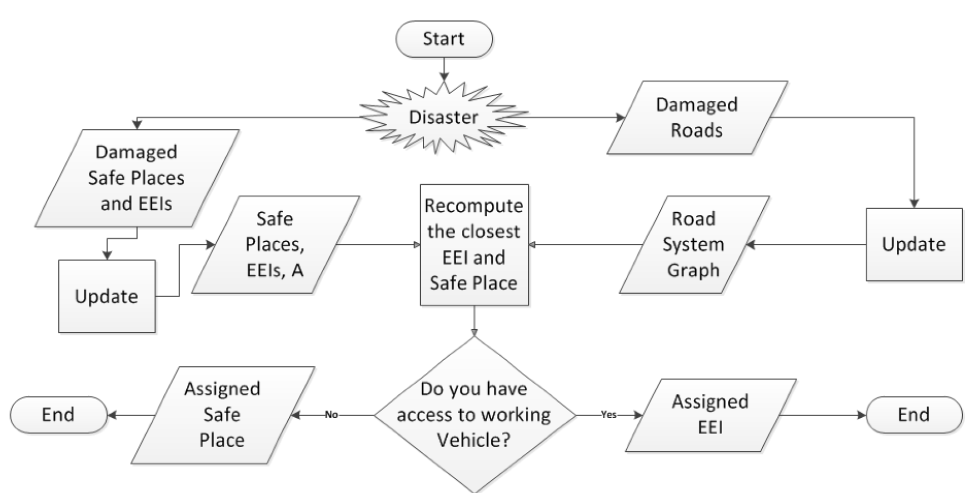
The proposed model randomly assigns departure times to evacuees and their routes based on the shortest path algorithm. Our emphasis, however, is more on the modeling and simulation of traffic. The evacuees will obey traffic laws at intersections, as assumed by the model. The proposed model does not account for other behavior patterns, such as panic. Currently, the model precomputes the assigned routes, but dynamic reassignment capability can be added because all necessary data are stored in a clearly defined and advertised data structure that allows modularity of implementation. Hence, condition three is partially met. That said, the proposed method is shown in Figure 1.
3.2. Model Assumptions
The proposed model can simulate traffic over large geographical areas that include several cities and towns. It is scalable to even larger geographic areas, like a state, if provided with the corresponding data, thus meeting condition four. It can also simulate the evacuation over multiple days, thus meeting condition five. Allowing model operators to evaluate “what-if” scenarios requires some modification that is not expected to be difficult and is indeed the main objective of this research.
The simulation runs under the following assumptions:
- (1)
- Once people leave the County, they are safe.
- (2)
- No one enters the County during the evacuation time.
- (3)
- People who do not have access to a working vehicle will meet at the nearest school, where buses or similar public transit vehicles will pick them up.
- (4)
- Schools are assumed to be safe place destinations.
- (5)
- People are at home when the evacuation is ordered. This is a good assumption if the evacuation starts at night. If the emergency occurs suddenly in the middle of the day, then a large proportion of people may be at work and may have to go home to pick up or meet with their families before actually evacuating. This will complicate the simulation.
- (6)
- The time at which a vehicle begins the evacuation journey is exponentially distributed with a mean of 40 min.
- (7)
- All the connection matrices are built based on the assumption that U-turns are not allowed, except for dead-end intersections.
- (8)
- One traffic direction for a bidirectional road segment is assumed to be independent of the opposite traffic direction for the same road segment.
- (9)
- The capacity of a sink place is assumed infinite.
- (10)
- Once a person/vehicle passes the intersection where the intended target is located, the person is considered to have arrived at the target. The time from the intersection at the target is neglected.
- (11)
- People are assumed to be rational and will comply with the evacuation order, will go to the assigned destination using the shortest route (assumed to be the same as the assigned route), and will comply with traffic laws.
- (12)
- When the evacuation starts, there is no significant traffic on the streets.
- (13)
- No psychological factors, such as panic, are considered. Panic can perhaps be expected to be limited since people evacuating using vehicles have minimal face-to-face contact.
- (14)
- All the intersections have commensurate service rates.
- (15)
- Unless it is clear from the context, “person” or “vehicle” are used interchangeably. The distinction would be needed if the person is driving a vehicle with other riders, typically family members or friends.
- (16)
- Intersection arrival rate, road arrival rate, and road service rate are assumed to be deterministic and equal.
- (17)
- On an uncongested road segment, vehicles will move at a speed close to the indicated speed limit.
- (18)
- No platoon-type behavior or congested on busy road segments was included.
Most of the above-mentioned assumptions can be relaxed without greatly impacting the model, even though the simulation results, such as the evacuation time, may be adversely affected. Assumption 11 (about panic and other psychological effects) would be difficult to lift and may require a significantly different approach. Some assumptions, including 2, 4, 5, 6, 7, 10, 12, and 15, can be easily lifted with more effort in the future and information. Assumption 18 can be lifted with some effort in the future to include platoon and congested dynamics based on vehicle density per unit of road length. Still, the proposed model significantly contributes to the field. First, an accurate highway system model is created directly from shapefiles, which could be used as a base for many applications and activities in many transportation and urban engineering fields. This, to the best of our knowledge, has not been done before and achieved such accurate results. Second, a mesoscopic simulation model is developed that meets most of Chiu et al.’s requirements. Third, the model is populated automatically from the shapefiles and other data, such as a list of addresses in a geographic area, which was not well addressed in the previous studies and will be beneficial in many applications. Finally, the model is used to illustrate the evacuation of Guilford County after an after-hour attack, and statistics and problematic patterns (such as congestion points) are identified.
3.3. Modeling a 4-Way Intersection Using a Petri Net
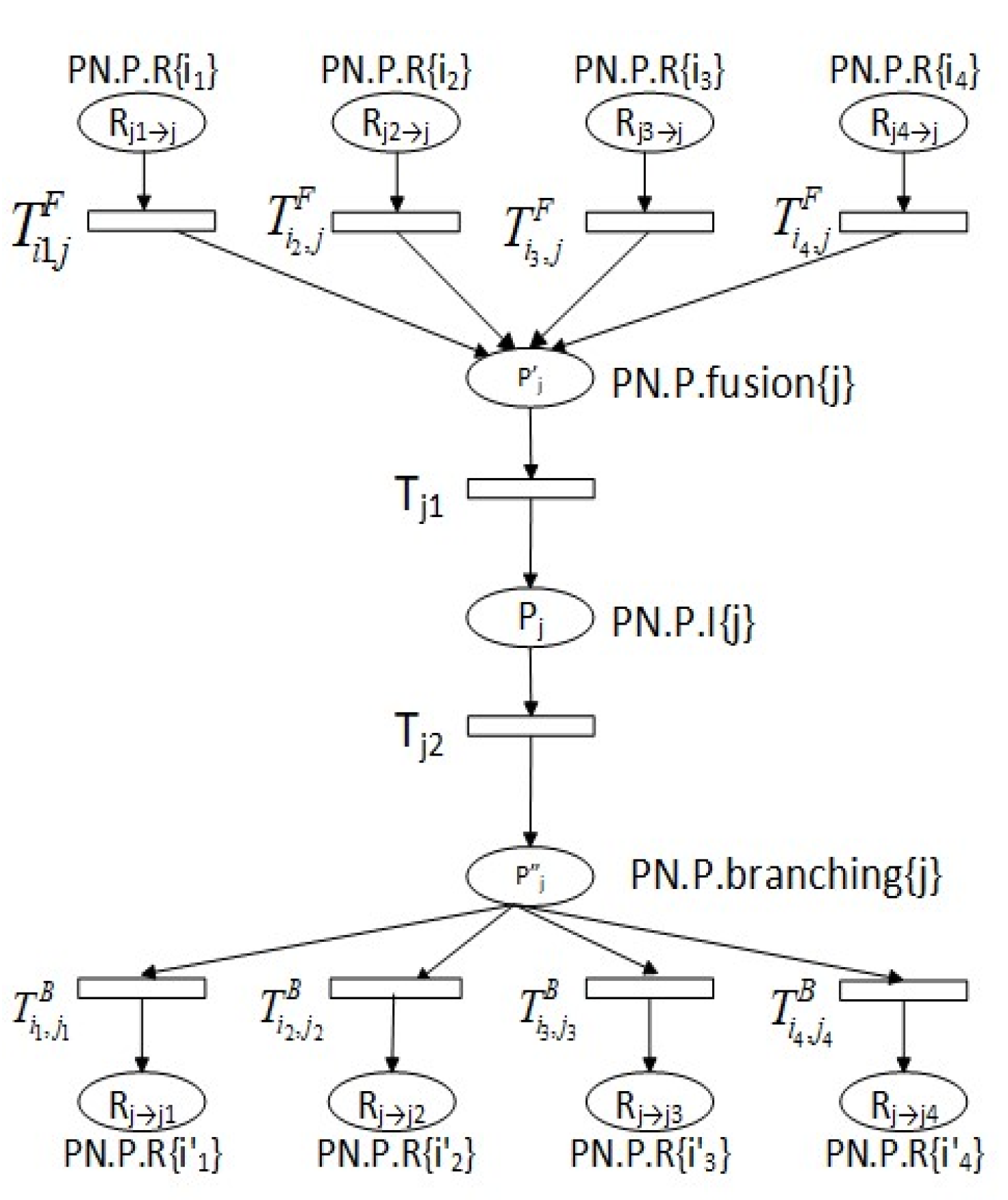
The basic idea is that an intersection can be represented by a Petri net with three places (fusion, hold, and branching). Each intersection includes one random queue with one server that will serve the vehicles and controls the efficiency of the intersection. Currently, a simple random delay is assumed. A road segment is also modeled as a queue with one or more servers depending on the number of lanes of the road. The road segment will serve the vehicles by moving them from their current intersection to the next intersection on their path to the destination. The service model here is largely deterministic based on the assumed speed that is related to the vehicular density.
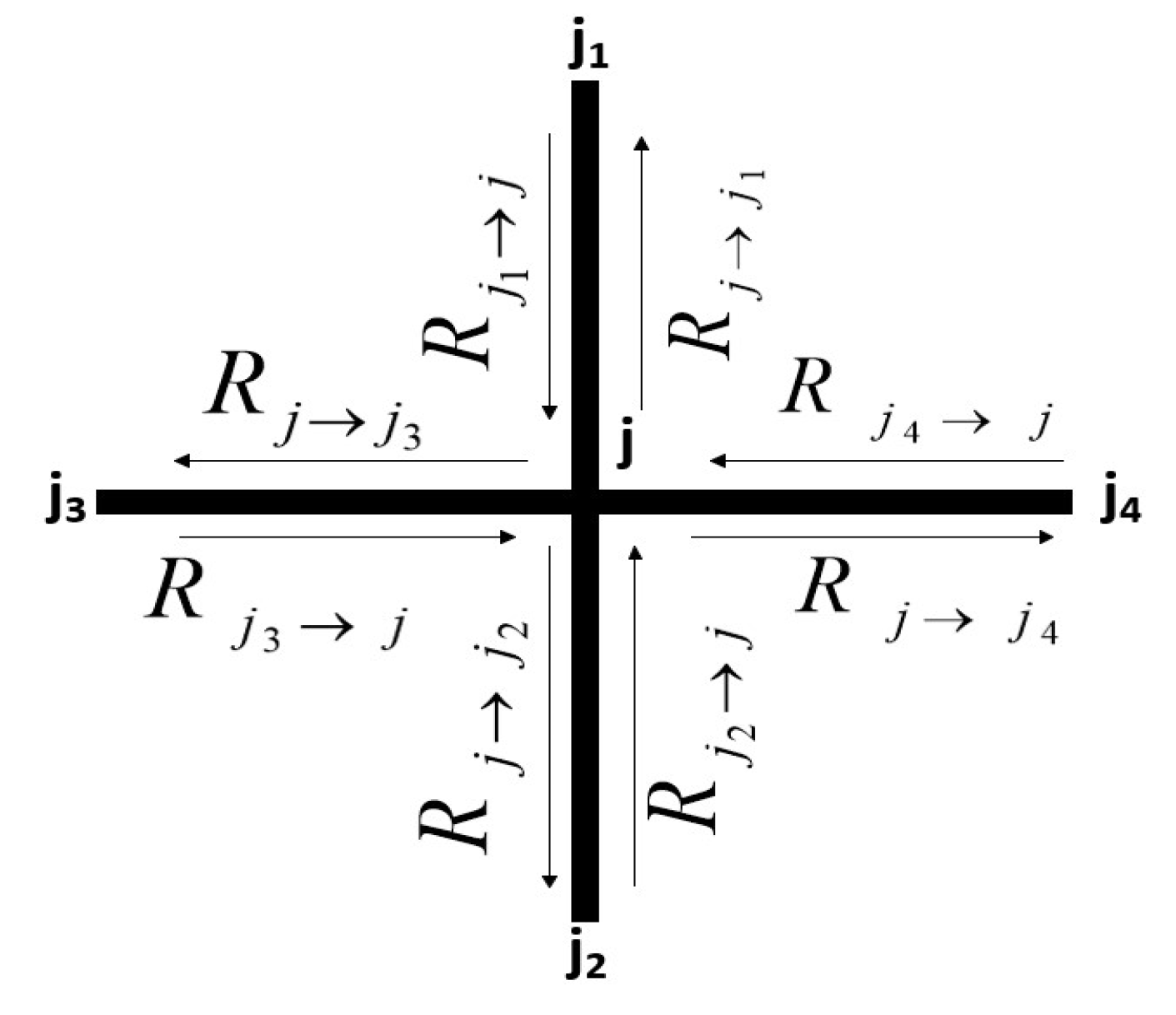
We present a Colored Deterministic and Stochastic Petri Net (CDSPN) model for a 4-way intersection j. A typical 4-way intersection, as shown in Figure 2, consists of four incoming traffic flows (Rj1→j, Rj2→j, Rj3→j, Rj4→j) and four outgoing traffic flows (Rj→j1, Rj→j2, Rj3→j, Rj4→j). The intersection j can be modeled as a D/M/1/k queue. Therefore, arriving at the intersection is deterministic, while leaving the intersection is stochastic. The capacity of the intersection is finite, and the intersection has one server.
Figure 3 shows the CDSPN model for intersection j. The model has been built under the assumption that the inflows are independent of the outflows of the common intersections. The Petri net has places such as Rj1→j, which is an inflow place for intersection j and an outflow place for intersection j1. A vehicle in this place is driving from intersection j1 toward intersection j over the corresponding road segment of that flow.
Moreover, Pj is a fusion place where all the vehicles on the path to intersection j will aggregate and wait to enter the intersection. Pj is the Intersection-Hold (or I-Hold) place which represents a buffer that holds the vehicles under service by j. A vehicle is in Pj if a vehicle is crossing intersection j. Finally, Pj is the branching place that contains the vehicles that have been served by the intersection server and are transitioning (typically with zero wait time) to enter the next outflow place. Nonzero wait times occur only if there is congestion.
The Petri net transitions are denoted as follows: TFi1,j denotes a deterministic transition from an inflow place i1 (coming from road segment i1) to the fusion place Pj. TBi1,j1 denotes a deterministic from the branching place Pj to the outflow place i1 connected with road segment i1. Tj1 is a deterministic transition that controls the movement of vehicles from the fusion place Pj to the intersection holding place Pj. Tj1 may represent a traffic light, stop sign, yield sign, or any means of traffic regulation. Finally, Tj2 is a stochastic transition with rate µj(t) that controls the movement of vehicles from the I-Hold place Pj to the branching place Pj. Tj2 represents the server in the intersection queue model. µj(t) is the service rate of the intersection.
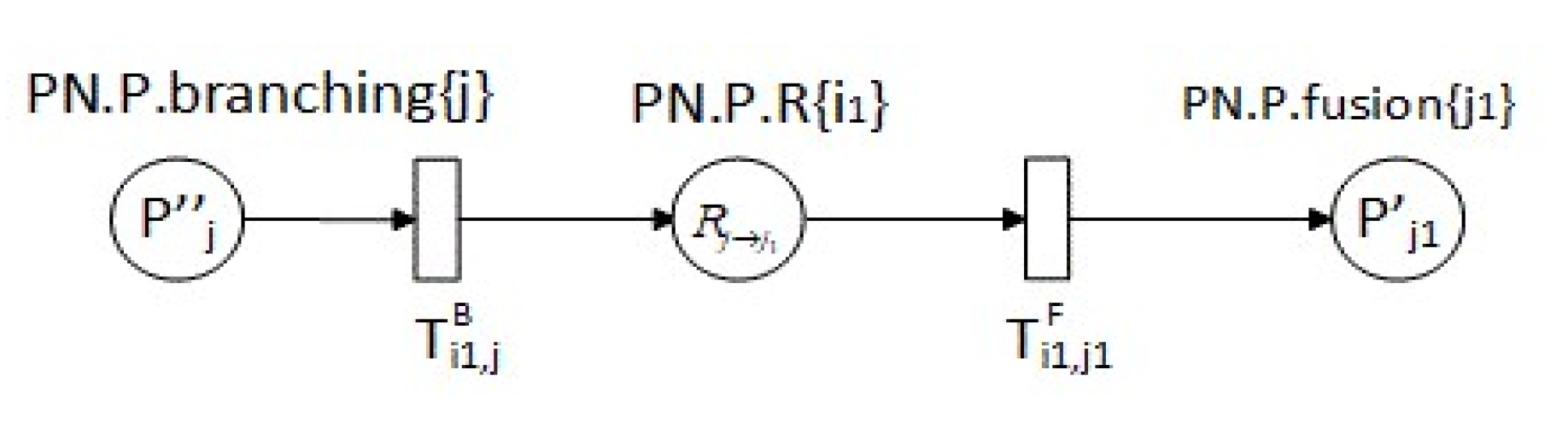
The road segment is modeled as a D/D/n/k queue for each direction of the road. Therefore, a one-directional road is modeled by one queue, and a bidirectional road is modeled by two queues. For instance, with reference to Figure 2, a bidirectional road segment i1, which links intersection j to j1, is modeled by two queues. Figure 4 exhibits the first queue of the flow Rj→j1, which models the traffic flow from intersection j to j1. The second queue of the flow Rj1→j is the opposite traffic flow of the road segment i1.
4. Description of Data Structures
For simulation purposes, we created the People Data Structure P, which defines a fictitious population for Guilford County. Simple assumptions were used to create this population. For instance, a small random number of residents are assigned to every address, which underestimates the number of people at businesses. This will be fixed in the future, but this currently reflects the assumption that the evacuation starts late at night, and perhaps after an evacuation call and hence after most people went back to their homes to prepare for the evacuation.
About one to three persons are randomly assigned to each address. Notable fields include: P.id(o) is a unique id for Person o, P.address(o) is the address on which Person o lives, P.status(o) where a person is randomly assigned a status like (‘Self-evacuee’, ‘Self-ambulance’, or ‘Transit-dependent’, or ‘Injured’) where we assumed that 10% of the population was injured, 9% needed public transit, and 81% were healthy and had access to cars.
P.target(o) is a precomputed evacuation target for o, assuming that the person’s status is ‘Self-transit’. If Person o has the status ‘Self-ambulance’, the target will be to the closest medical facility, and for ‘Transit-dependent’, the target will be to the closest predetermined Safe Place.
The Petri Net Structure (PN) is a dynamic structure that changes throughout the simulation, in contrast with the address and road data structures. Notable fields include PN.P for places, PN.S for sink places, PN.T for transitions, and PN.M for markings. Places include PN.P.fusion, PN.P.I, PN.P.branching, and PN.P.R corresponding to fusion place, intersection-Hold place, branching place, and road-Hold place, respectively. Each member of PN.P is a cell array that holds the indices of people who are driving at that place at time t. The size of PN.P.fusion, PN.P.I, and PN.P.branching is equal to the number of nodes in the Roads System graph (nb. intersections). However, the size of PN.P.R is equal to the number of links in the Roads System graph. An intersection on which a target is located has a sink place.
Figure 5 shows an intersection j whose IH2B (I-Hold to Branching) transition has two output places. The output places are the branching place and the sink place for target L. The PN.S field has one member (PN.S.Target), which is a sink place that holds the indices of people who have arrived at their target. Its size is equal to the number of targets.
Accounting for vehicles locations follows the following pattern: PN.P.X{j} = [k1, k2, …] means that people/vehicles whose indices are k1, k2, … are interacting with Intersection j where X can assume one of 4 values: I denotes vehicles currently in the intersection, branching indicates vehicles going out of the intersection, fusion indicates vehicles that are arriving to the intersection, R denotes vehicles in road segment j, and finally, target denotes vehicles that have arrived at their targeted destinations. In the above notation, there is no clear distinction between people and vehicles in the sense that we assume that every person of interest is in the proper vehicle. The model can be easily updated to relax this assumption.
The aim of PN.T is to map each transition to its corresponding output or input place. PN.T has four subfields. The first subfield is PN.T.branching, which maps TBi,j to its corresponding output place. The second subfield is PN.T.fusion, which maps TFi,j1 to its corresponding input place. The third subfield is PN.P.R, which maps each traffic flow with its corresponding road i into the road data structure R. Finally, the PN.T.Target subfield maps TBi,j to the corresponding sink place if there is a target located on that intersection j.
The transitions are accounted for using the following pattern: PN.T.X(k) = j means that when transition k fires, people will be moved from place X to the next place in the PN. For instance, if X is branching, people will be moved to a road-hold place, as shown in Figure 3. Similarly, X can also be fusion (moving from road-holds to fusion places), R (moving from a branching or fusion place to a road segment), and target (moving from a branching place to a sink place).
The markings are represented in the dynamic structure PN.M, which captures information about the location and status of vehicle o at the current time t. This information determines and is determined by the transitions. Notable subfields are currentRoad(o), currentIntersection(o), TimeToEnter(o), hasEntered(o), hasExited(o), distanceToGo(o), and speed(o), which are self-explanatory. The speed is computed by multiplying the speed limit of the road by a random number in the range [0.8, 1.2]. In short, we assume that people drive at 80% to 120% of the speed limit. Other models, such as the flow density, can be used.
4.1. Implementing the Transitions
The function B2RH implements the transitions TBi1,j1 (see Figure 3). At every time sample, one examines whether the conditions of such transition are met, such as (a) there is a vehicle in the branching place (enabled); (b) the vehicle is heading to corresponding flow (as indicated by PN.M.currentRoad which represents a color); and (c) the corresponding R-Hold has a room for more vehicles (not inhibited). If enabled, B2RH will compute how many vehicles can move, then will move the vehicle(s) from the branching place to the corresponding outflow R-Hold place by deleting vehicle(s) from PN.P.branching(j) and adding the same vehicle(s) to PN.P.R(i). Otherwise, the state does not change.
The function IH2B implements the transition Tj2 (see Figure 3). At every time sample, the function will examine the following conditions: (a) there is at least one vehicle in the IHold place, and (b) the corresponding branching place has room for more vehicles. Subsequently, IH2B will compute how many vehicles can move; then, the function will allow a vehicle to pass from the I-Hold according to probability. Here the service is stochastic and depends on the relevant average time delay m. In general, m depends on the intersection and the target branching place to reflect, for instance, that left turns introduce longer delays than right turns and that some intersections are slower than others. In the absence, however, of empirical data about intersections, the average delays are assumed to be practically the same for most intersections. The function will repeatedly draw from the queue until the number of vehicles that have moved is met. Finally, the function will move the vehicle(s) from the I-Hold place to the corresponding branching place by deleting the vehicle(s) IDs from PN.P.I(j) and adding the same vehicles IDs to PN.P.branching(j).
The function F2IH is the guard function for the transition Tj1, as illustrated in Figure 3. At every sampling time, the function will examine if the transition has met the conditions: (a) there is a vehicle in the Fusion place, and (b) the corresponding I-Hold place has room for more vehicles, indicating that the transition is not inhibited. Subsequently, F2IH will determine how many vehicles can move and will move the required number of vehicle(s) in the head of the Fusion place (a FIFO policy) to the corresponding I-Hold place by deleting the IDs of the vehicle(s) from PN.P.fusion(j) and adding the same vehicles IDs to PN.P.I(j). If not, the Petri net will remain unchanged.
The function RH2F is the guard function for the transition TFi1,j (see Figure 3). At every time sample, the function will fire if (a) there is a vehicle in the R-Hold place and that vehicle has PN.M.DistanceToGo(o) = 0 (meaning that this vehicle has crossed the road); and (b) the corresponding Fusion place has room for more vehicles. Subsequently, RH2F will determine how many vehicles can move, then will move the vehicle(s) from the R-Hold place to the corresponding Fusion place by deleting the vehicle(s) from PN.P.R(i)and add the same vehicles to PN.P.fusion(i). If not, the state of the net will remain unchanged. PN.M.currentIntersectio (color) for the moved vehicle(s) will get updated in this function.
4.2. Main Simulation Loop
To perform empirical analysis, we use synchronous simulation. In other words, markings and transitions are updated according to a sampling clock, typically every second. The four major types of transitions in the Colored Deterministic and Stochastic Petri Net (CDSPN) are Fusion to I-Hold (F2IH), I-Hold to Branching (IH2B), Branching to R-Hold (B2RH), and R-Hold to Fusion (RH2F). The PN of every intersection consists of three places (Fusion, I-Hold, Branching) and two transitions (F2IH and IH2B). The PN of every road consists of one place (R-Hold) and two transitions (B2RH and RH2F). The following tasks are completed within the main loop:
- (1)
- Update the list of vehicles that are currently in the highway system. This includes identifying vehicles that are entering the highway system at this time and placing them in the correct R-Hold places, updating the list of people/vehicles that are tracked, and removing those who arrived at their targets.
- (2)
- Terminate the simulation if all people have arrived at their targets or by some other condition.
- (3)
- Update the distance to go (to the next intersection) along the assigned path for every tracked vehicle.
- (4)
- Loop over the intersections and move people through them by calling the transition functions B2RH, IH2B, F2IH, and RH2F in sequence.
- (5)
- Loop over all roads and move people according to some velocity profile.
5. Simulation Results
The model was tested by simulating the evacuation of Guilford County (GC) in North Carolina. The model, however, is useful for other applications. The Petri net includes 35,476 places and 43,540 transitions with 531,595 tokens (markings), where each token represents a person/vehicle in GC. The evacuation took about 8.7 h, and the bottlenecks of the evacuation were identified. This section discusses and explains the results of the simulation of the evacuation of the GC population to their targets. The simulation runs until every vehicle in the system has arrived at its assigned target. In the first simulation conducted, a sampling time of Ts = 1 s was used. The last vehicle to enter the system did so after 4 h, and the last vehicle exited after 8.77 h. We repeated the simulation with Ts = 10 s, and the corresponding times were 5.5 h and 8.7 h. Snapshots of the system states were stored every 120 s for Ts = 1 s and every 1200 s for T = 10 s.
5.1. Following a Vehicle
To examine the simulation results, as well as the type of information that can be gained from the simulation, we follow a randomly selected person/vehicle. For simplicity, we will refer to a person whose P.id = 114,359 as John, the target P.target is denoted 3, which means that he has to evacuate to the nearest exit point, the address P.address = 65,658, and the status P.status is “Self-transit”. The simulation showed that John entered the highway system at 3995 s after the start of the simulation. The closest snapshot after John entered the system is taken at time 4080 s.
Table 1 provides the dynamics of John’s information until he reaches his target. The first row of the table includes the initial state for John, which includes the intersection and the road flow from where John will start driving. The table shows some of the intersections and the roads that John uses along the way to his target. John needed about 30 min to reach his target.
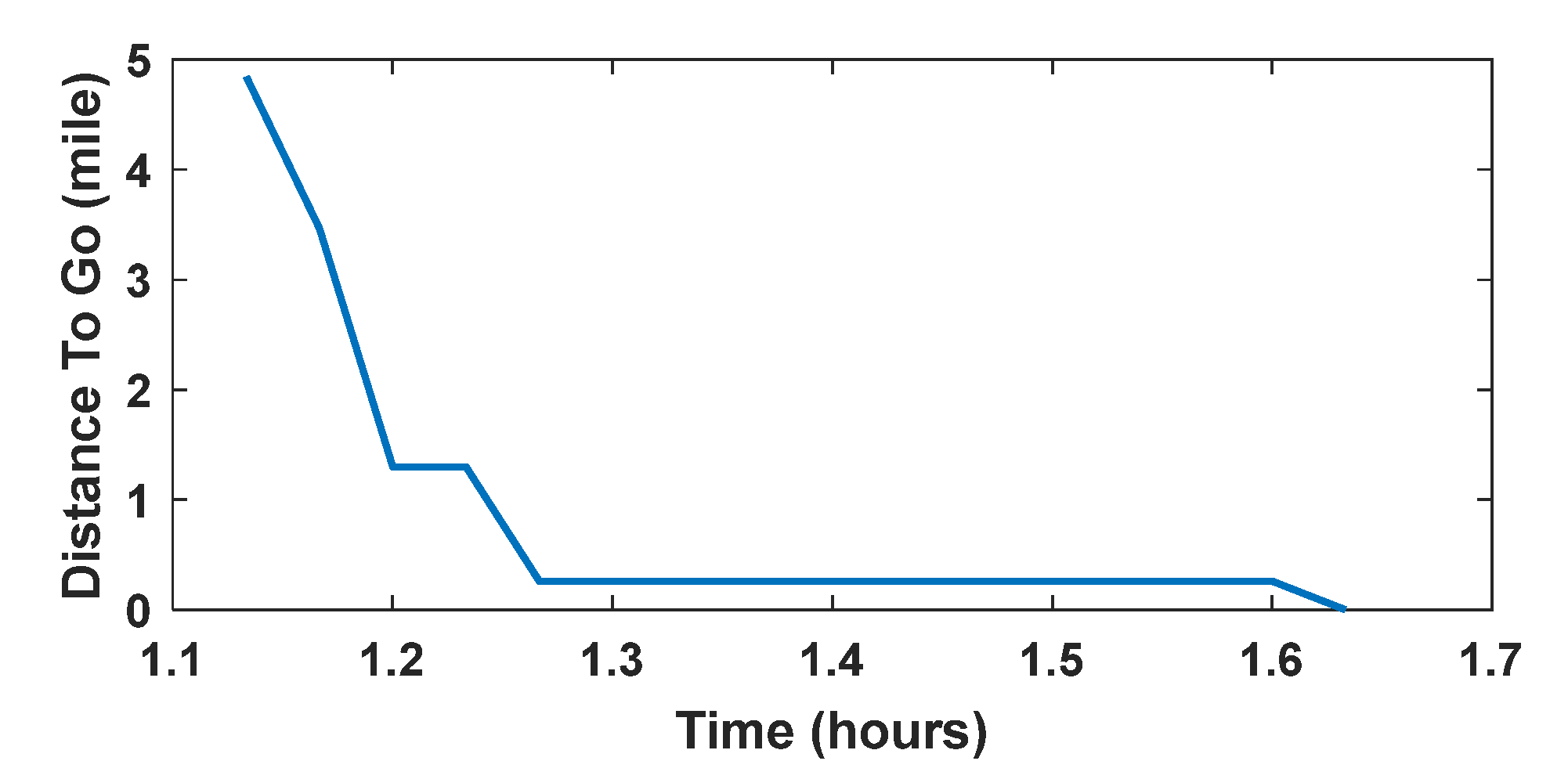
Furthermore, Table 1 reveals that John faced congestion at Intersection 3165, where John needed about 20 min to leave the branching place of the intersection. Such a situation is expected to happen during the evacuation since everyone is competing to evacuate. Intersection 3165 is the intersection of an urban road with NC State 62. John tries to merge with the highway traffic, where priority is given to the traffic on the highway. Therefore, the traffic on the urban road is expected to face extra delays. So, the CDSPN model has the ability to locate the congestion nodes in the roads network system. The distance that John needs to drive to his target is 4.85 miles.
Figure 6 reveals the distance that John has covered at every timestamp. The figure shows that John needs about half an hour to arrive at his target. John had to stop at one intersection at 1.2 h (after the start of evacuation) for about 2 min. Moreover, he faced congestion in clearing two intersections, which consumed 20 min of his time. Therefore, for 73% of the time, John was waiting to clear two intersections, driving at a reasonable speed only for 27% of the time.
5.2. Following a Group of People Living around the Same Intersection
The dynamics of a group of people living around the same intersection will be examined. For example, Intersection 826 is located in the northwest of the GC. There are 20 persons living immediately close to this intersection, and their targets are (2 persons ‘Self-ambulanced’, 4 persons ‘Transit-dependent’, and 14 persons ‘Self-transit’.
Table 2 exposes the paths for three classes of people (1) Self-ambulanced, (2) Transit-dependent, and (3) Self-transit. The path to class 1 (closest hospital) splits early on the second intersection (5078). This path is almost independent of the paths of the other two classes of people. Classes 2 and 3 are sharing most of the route. They split at intersection 3083, as shown in Table 2. Moreover, the table includes the meantime of evacuation for each target of the group.
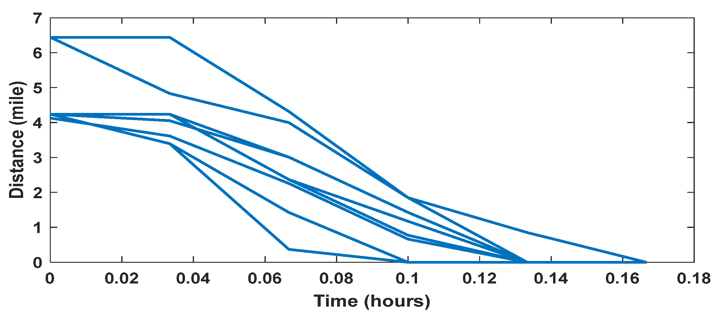
Figure 7 shows the distance that 14 people in class 3 ‘Self-transit’ cover over time. The starting times for different people are shifted to zero to facilitate comparison. The lines overlap for the people who share the same route or part of the route at the same time. The distance for the people who are heading to class 1 is the longest, and so is their travel time. However, the travel time for the other two classes is almost the same.
5.3. Tracking the Whole Population of GC
The dynamics of the whole population of GC will be examined. The population is divided into three different classes based on the corresponding targets. The number of people in each class in GC is 53,110 persons ‘Self-ambulanced’, 48,057 persons ‘Transit-dependent’, and 430,428 persons ‘Self-transit’.
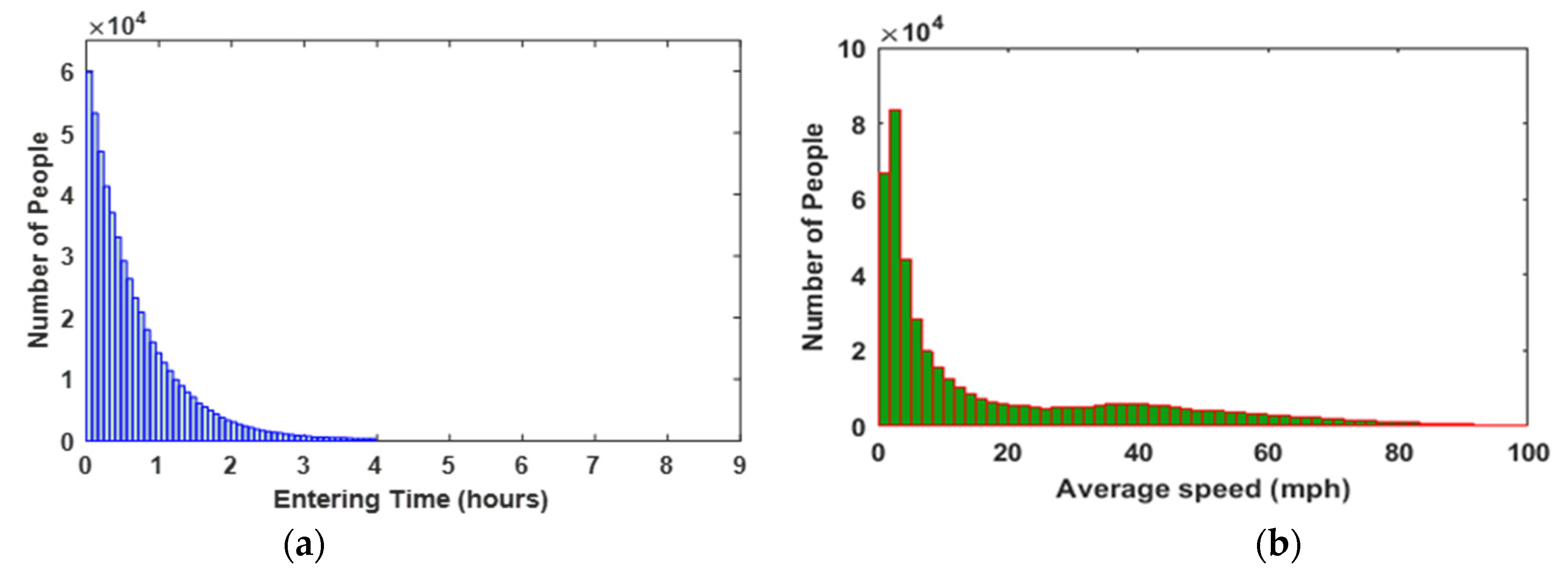
Once the evacuation alert takes place, people will start to leave their homes at randomly assigned times, reflecting that individual reaction time will vary. Many of them will leave right away, while others will need longer or may not leave at all. A random, exponentially distributed time with an average of 40 min is assigned to each person in GC as an entering time. Figure 8a demonstrates how many people will enter the system over different periods of time. By the second hour of the simulation, the majority of the population has entered the system. In contrast, the rest of the population enters the system over the next two hours of the simulation.
After entering the system, people start to drive to their targets. Individual driving speeds on an uncongested road segment will be based on the speed limit of the road segment and will range between 80% and 120% of the speed limit. The overall average speed for each person is computed based on the distance and the travel time to the target. The travel time includes waiting and congestion times. Figure 8b shows the distribution of people’s overall average speeds. Most of the people have an overall average speed of less than 20 mph. Therefore, most people have faced significant congestion along the way to their targets.
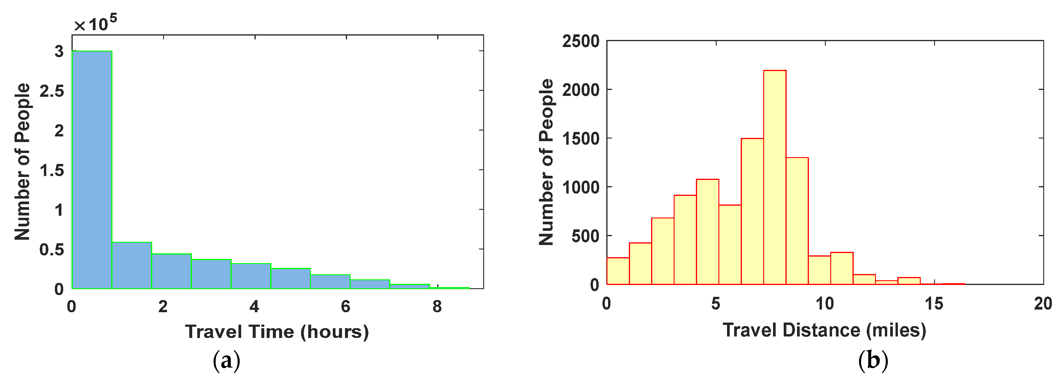
The fact that most of the people have 20 mph as an average speed demands additional scrutiny. About 300,000 vehicles will arrive at their targets in less than 1 h, as shown in Figure 9a. The mean travel time for the whole population is 1.53 h. However, a minority of the people needed more than 4 h to reach their targets. Such time is relatively high when compared to the average travel time.
The travel distance from starting addresses to the targets is also examined. Self-transit people are expected to have the longest travel distance because they have to leave the county. The mean travel distance is 7.35 miles for this group. The mean distance is slightly higher than 1/4th of the longest side of GC. The people heading to exit points are grouped based on their travel distance in Figure 9b.
The exit time for a person is the time when that person leaves the county, indicating that this person has arrived at his/her target. As can be seen in Figure 10a, many people will exit the system after the first hour of the emergency warning. The time needed for the whole population to arrive at their targets was less than 9 h, which is longer than the travel considering that some people will enter the system quite late, as described above. The mean exit time for overall vehicles is 2.19 h.
The number of people who pass through the intersections is shown in Figure 10b. The figure is sorted from the intersections with the highest usage to the intersections with the lowest usage. The figure shape shows an exponential decay. Isolated intersections will get little usage, while major intersections are heavily used and often congested. The exit points will get the highest usage.
5.4. Visualization of Self-Transit Evacuees
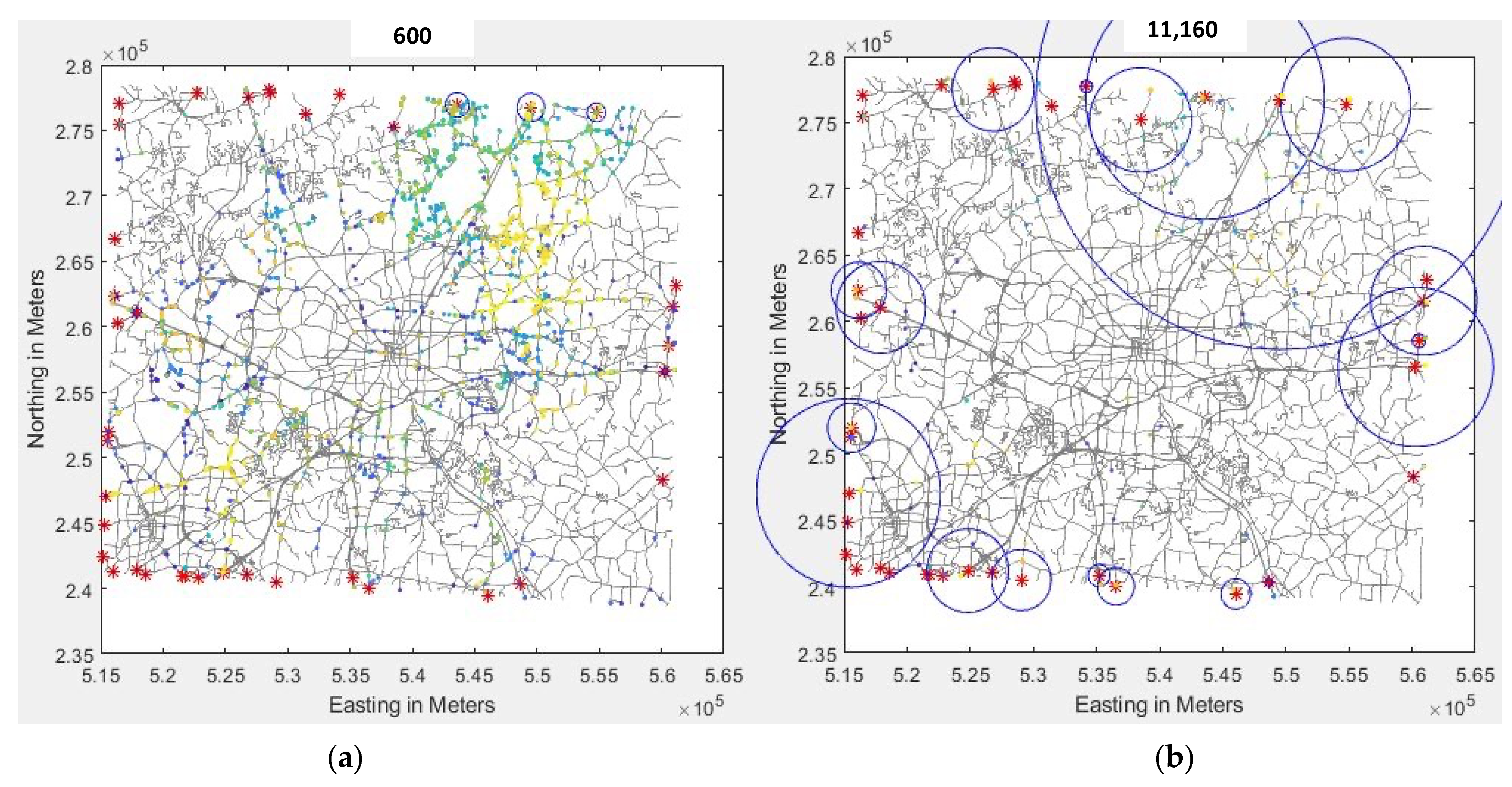
To visualize the movement of the population along with the highway system during the evacuation, a sample of 10,000 self-transit people is randomly chosen to create a movie. In the movie, each person is represented by a colored dot, and the Evacuation Exit Intersection (EEI) is represented by red stars. Around the used EEI, a blue circle is drawn. The size of the blue circle is scaled based on the number of people who use that EEI. When the movie starts, people are assumed to be at their home addresses. The EEIs are highlighted with red stars on the borders of the GC; no blue circle is shown since no one has exited yet.
Figure 11 shows the evacuees moving along the roads system. Figure 11a displays the state of the system 600 s after the start of the simulation. At the top of the figure, the timestamp of the snapshot is shown. Small blue circles appear around some EEIs. The circles are small because few people have arrived at their target. The blue circles grow bigger as more people arrive at their targets. In the state of the system after 2520 s of the start of the simulation, more people are getting on the roads, and the distribution of the evacuees among the EEIs is not uniform. After 11,160 s, most of the evacuees have arrived at their targets, as shown in Figure 11b. NC 29 N, I-40 E, and I-40 W businesses have large blue circles, which means that they are mostly used during the evacuation.
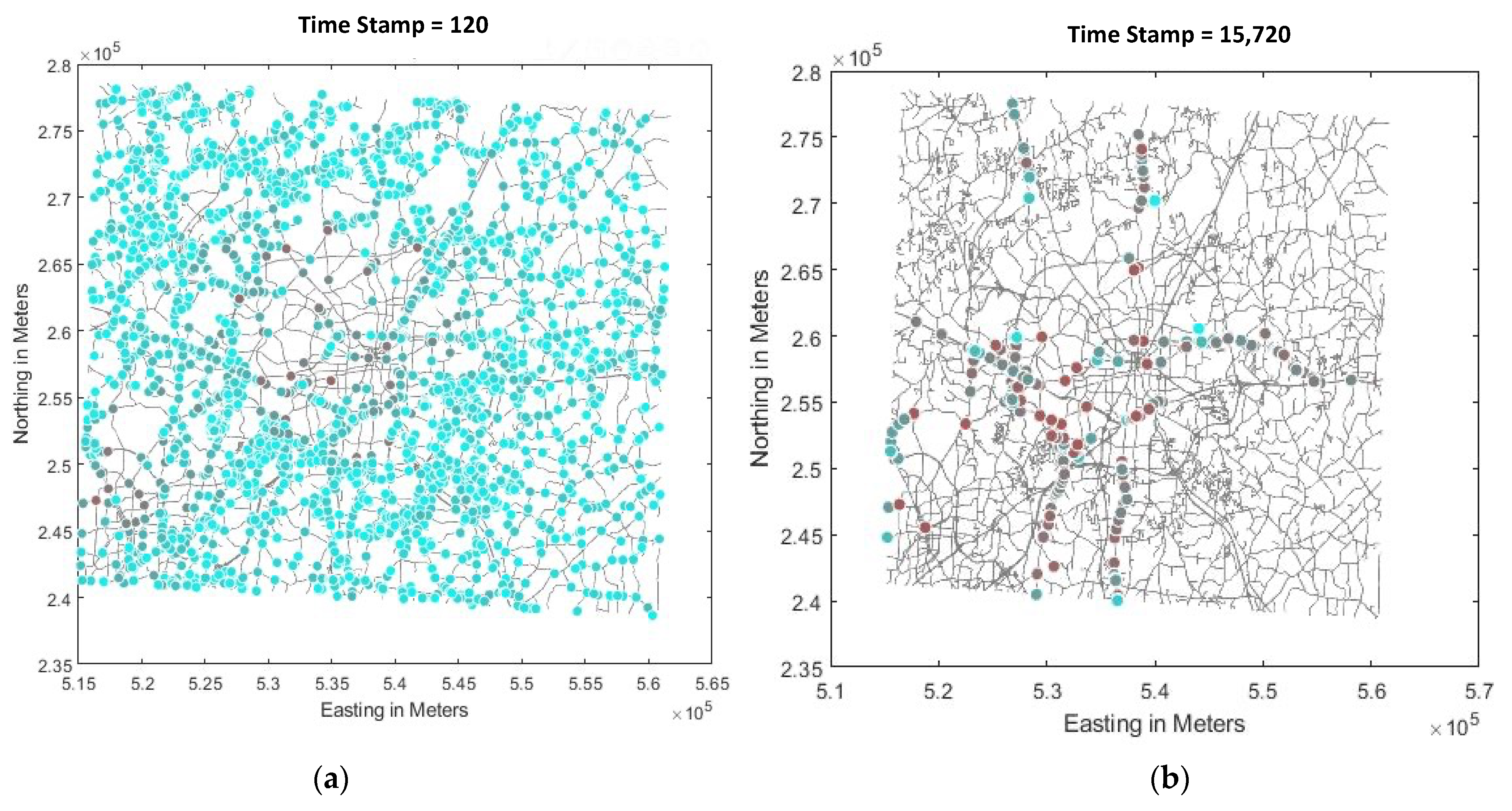
5.5. Visualizing the Traffic on Intersections
To visualize the traffic load on intersections during the evacuation, a movie is created based on the snapshots that have been taken during the evacuation of the GC population. When there is traffic at the intersection, a colored circle is drawn; otherwise, nothing will be drawn. The heavier the traffic, the darker the color. A circle disappears when the intersection becomes empty. A dark brown circle means that the traffic at that intersection is very heavy. Figure 12a shows the traffic at the intersections when the time is 120 s. Most of the intersections have light blue circles on them, which means that the traffic on them is light. Figure 12b shows clearly which roads are congested. Wendover E, Wendover W, I-40 E, I-40 W, and others are the congested roads. These roads are expected to be congested since these roads are primarily used roads or are Interstate roads.
6. Conclusions
We developed a mesoscopic modeling and simulation approach for modeling traffic flow over a large geographic area where people at addresses are assigned to vehicles, and their destinations and routes are computed. The approach is partly microscopic in the sense that individual vehicles are simulated and macroscopic in the sense that the highway system and vehicle interactions are simplified. To make the simulation specific, we considered the scenario in which most people self-evacuate GC through the closest exit points over the shortest path. Dijkstra’s algorithm is used to compute the shortest paths.
We also developed an automatic method to assemble the Petri net that represents the evacuation of Guilford County (GC). The Petri net includes 35,476 places and 43,540 transitions with 531,595 tokens, where each token represents a single person in GC. We simulated the evacuation and developed statistics and evaluations for the results. From the simulation, the evacuation took about 8.7 h, and most of the population entered the system in the first 2 h. The distribution of people’s overall average speeds has two peaks at 20 mph and 40 mph. The mean travel time for the whole population is 1.53 h. However, a minority of the people needed more than 4 h to reach their targets. The mean travel distance is 7.35 miles for self-transit people.
The mean of the exit time overall vehicles is 2.19 h. The usage of intersections has an exponential distribution. Isolated intersections will get a small number of users, while major intersections will get more usage. The exit points will get the highest usage. We have created two movies. The first movie visualizes the movement of a sample of 10,000 self-transit people who are randomly picked up along the highway system. The distribution of the evacuees among the EEIs is not uniform. NC 29 N, I-40 E, and I-40 W business are mostly used during the evacuation. The second movie visualizes the traffic load at intersections during the evacuation. From this movie, it can be noted that Wendover E, Wendover W, I-40 E, I-40 W, and others are the congested roads. These roads are expected to be congested since these roads are primarily used roads or are Interstate roads. For future work, first, considering emergency tasks, such as rescuers, volunteers, organizers, and some agents who have to cooperate with other agents, if necessary, will add to the paper. Second, considering a different geographical location will also enrich and validate the model. Proposing the model was the first step in this study, and we plan to use a different dataset considering the results of this study as a baseline. Another way that we will investigate is to reproduce results from previous studies for comparison purposes.
Author Contributions
Conceptualization, H.Q. and M.B.; methodology, H.Q., M.I.A. and M.B.; software, H.Q. and M.I.A.; validation, H.Q. and M.I.A.; formal analysis, H.Q. and M.I.A.; investigation, H.Q. and M.I.A.; resources, H.Q. and M.I.A.; data curation, H.Q. and M.I.A.; writing—original draft preparation, H.Q., M.I.A. and M.B.; writing—review and editing, M.B. and H.I.A.; visualization, H.Q., M.I.A. and H.I.A.; supervision, M.B.; project administration, M.B. and H.I.A. All authors have read and agreed to the published version of the manuscript.
Funding
This research received no external funding.
Data Availability Statement
The data presented in this study are available on request from the corresponding author.
Conflicts of Interest
The authors declare no conflict of interest.
References
- Song, W.; Zhu, L.; Li, Q.; Wang, X.-D.; Liu, Y.; Dong, Y.-C. Evacuation Model and Application for Emergency Events. In Proceedings of the 2009 Fourth International Conference on Computer Sciences and Convergence Information Technology, Seoul, Korea, 24–26 November 2009; pp. 1325–1329. [Google Scholar]
- Robinson, R.M.; Khattak, A. Route change decision making by hurricane evacuees facing congestion. Transp. Res. Rec. 2010, 2196, 168–175. [Google Scholar] [CrossRef] [Green Version]
- Von Neuman, J.; Burks, A.; Gardner, M.; Wolfram, S.; Wolfram, S.; Sipper, M.; Wolfram, S.; Wolfram, S.; Wolfram, S.; Baldwin, J.; et al. Theory of Self Reproducing Automata; University of Illinois Press: Urbana, IL, USA, 1966. [Google Scholar]
- Chen, B.; Cheng, H.H. A review of the applications of agent technology in traffic and transportation systems. IEEE Trans. Intell. Transp. Syst. 2010, 11, 485–497. [Google Scholar] [CrossRef]
- Santos, G.; Aguirre, B.E. A Critical Review of Emergency Evacuation Simulation Models. Disaster Res. Cent. 2004. Available online: http://udspace.udel.edu/handle/19716/299 (accessed on 15 September 2022).
- Cova, T.J.; Johnson, J.P. A network flow model for lanebased evacuation routing. Transp. Res. Part A Policy Pract. 2003, 37, 579–604. [Google Scholar] [CrossRef]
- Ren, C.; Yang, C.; Jin, S. Agent-Based Modeling and Simulation on Emergency Evacuation. In International Conference on Complex Sciences; Springer: Berlin/Heidelberg, Germany, 2009; pp. 1451–1461. [Google Scholar]
- Wang, C.; Wang, J.; Bao, Q. A Cellular Automaton Model Based on Dynamic Floor-Field for Evacuation Process with Multi-Egress. In Proceedings of the 2014 IEEE International Conference on Systems, Man, and Cybernetics (SMC), San Diego, CA, USA, 5–8 October 2014; pp. 930–934. [Google Scholar]
- Vihas, C.; Georgoudas, I.G.; Sirakoulis, G.C. Cellular automata incorporating follow-the-leader principles to model crowd dynamics. J. Cell. Autom. 2013, 8, 333–346. [Google Scholar]
- Di Febbraro, A.; Giglio, D.; Sacco, N. A Deterministic and Stochastic Petri Net Model for Traffic-Responsive Signaling Control in Urban Areas. IEEE Trans. Intell. Transp. Syst. 2015, 17, 510–524. [Google Scholar] [CrossRef]
- Yuan, S.-X.; An, Y.-S.; Zhao, X.-M.; Fan, H.-W. Modeling and Simulation of Dynamic Traffic Flows at Non-Signalized t-Intersections. In Proceedings of the 2009 2nd International Conference on Power Electronics and Intelligent Transportation System (PEITS), Shenzhen, China, 19–20 December 2009; Volume 2, pp. 1–5. [Google Scholar]
- Wang, J.; Jin, C.; Deng, Y. Performance Analysis of Traffic Networks Based on Stochastic Timed Petri Net Models. In Proceedings of the Fifth IEEE International Conference on Engineering of Complex Computer Systems (ICECCS’99) (Cat. No. PR00434), Las Vegas, NV, USA, 18–21 October 1999; pp. 77–85. [Google Scholar]
- Chiu, Y.-C.; Zheng, H.; Villalobos, J.A.; Peacock, W.; Henk, R. Evaluating Regional Contra-Flow and Phased Evacuation Strategies for Texas Using a Large-Scale Dynamic Traffic Simulation and Assignment Approach. J. Homel. Secur. Emerg. Manag. 2008, 5, 1. [Google Scholar] [CrossRef]
- Bellemans, T.; De Schutter, B.; De Moor, B. Models for traffic control. J. A 2002, 43, 13–22. [Google Scholar]
- Kabir, S.; Papadopoulos, Y. Applications of Bayesian networks and Petri nets in safety, reliability, and risk assessments: A review. Saf. Sci. 2019, 115, 154–175. [Google Scholar] [CrossRef]
- Yin, D.; Wang, S.; Ouyang, Y. ViCTS: A novel network partition algorithm for scalable agent-based modeling of mass evacuation. Comput. Environ. Urban Syst. 2020, 80, 101452. [Google Scholar] [CrossRef]
- Hwang, Y.; Heo, G. Development of a radiological emergency evacuation model using agent-based modeling. Nucl. Eng. Technol. 2021, 53, 2195–2206. [Google Scholar] [CrossRef]
- Wu, W.; Li, J.; Yi, W.; Zheng, X. Modeling Crowd Evacuation via Behavioral Heterogeneity-Based Social Force Model. IEEE Trans. Intell. Transp. Syst. 2022, 23, 15476–15486. [Google Scholar] [CrossRef]
- Kaur, N.; Kaur, H. A Multi-agent Based Evacuation Planning for Disaster Management: A Narrative Review. Arch. Comput. Methods Eng. 2022, 29, 4085–4113. [Google Scholar] [CrossRef]
- Di Gangi, M. Modeling Evacuation of a Transport System: Application of a Multimodal Mesoscopic Dynamic Traffic Assignment Model. IEEE Trans. Intell. Transp. Syst. 2011, 12, 1157–1166. [Google Scholar] [CrossRef]
- Kubisch, S.; Stötzer, J.; Keller, S.; Bull, M.T.; Braun, A. Combining A Social Science Approach and GIS-Based Simulation to Analyse Evacuation in Natural Disasters: A Case Study in the Chilean Community of Talcahuano. In ISCRAM. (May 2019). Available online: https://www.researchgate.net/publication/333430720_Combining_a_social_science_approach_and_GIS-based_simulation_to_analyse_evacuation_in_natural_disasters_A_case_study_in_the_Chilean_community_of_Talcahuano (accessed on 15 September 2022).
- Gaddouri, R.; Brenner, L.; Demongodin, I. Controlled Triangular Batches Petri Nets for Hybrid Mesoscopic Modeling of Traffic Road Networks Under VSL Control. In Proceedings of the 2016 IEEE International Conference on Automation Science and Engineering (CASE), Fort Worth, TX, USA, 21–25 August 2016; pp. 427–432. [Google Scholar]
- Riouali, Y.; Benhlima, L.; Bah, S. An Integrated Turning Movements Estimation to Petri Net Based Road Traffic Modeling. J. Sens. Actuator Netw. 2019, 8, 49. [Google Scholar] [CrossRef] [Green Version]
- Ng, K.M.; Reaz, M.B.I.; Ali, M.A.M. A review on the applications of petri nets in modeling, analysis, and control of urban traffic. IEEE Trans. Intell. Transp. Syst. 2013, 14, 858–870. [Google Scholar] [CrossRef]
- Tolba, C.; Lefebvre, D.; Thomas, P.; El Moudni, A. Continuous Petri Nets Models for the Analysis of Traffic Urban Networks. In Proceedings of the 2001 IEEE International Conference on Systems, Man and Cybernetics. e-Systems and e-Man for Cybernetics in Cyberspace (Cat. No. 01CH37236), Tucson, AZ, USA, 7–10 October 2001; Volume 2, pp. 1323–1328. [Google Scholar]
- Badamchizadeh, M.; Joroughi, M. Deterministic and Stochastic Petri Net for Urban Traffic Systems. In Proceedings of the 2010 the 2nd International Conference on Computer and Automation Engineering (ICCAE), Singapore, 26–28 February 2010; 5, pp. 364–368. [Google Scholar]
- Makela, M.; Lahtinen, J.; Ojala, L. Performance Analysis of Traffic Control Systems Using Stochastic Petri Nets, Helsinki University of Technology, Digital Systems Laboratory, Helsinki, Finland. Ser. B Tech. Rep. 19 1998. Available online: https://research.aalto.fi/en/publications/performance-analysis-of-a-traffic-control-system-using-stochastic (accessed on 15 September 2022).
- Ashqer, M.I.; Ashqar, H.I.; Elhenawy, M.; Almannaa, M.; Aljamal, M.A.; Rakha, H.A.; Bikdash, M. Evaluating a Signalized Intersection Performance Using Unmanned Aerial Data. arXiv 2022, arXiv:2207.08025. [Google Scholar] [CrossRef]
- Basile, F.; Chiacchio, P.; Teta, D. A hybrid model for real time simulation of urban traffic. Control Eng. Pract. 2012, 20, 123–137. [Google Scholar] [CrossRef]
- Dotoli, M.; Fanti, M.P. An urban traffic network model via coloured timed Petri nets. Control Eng. Pract. 2006, 14, 1213–1229. [Google Scholar] [CrossRef]
- Demongodin, I. Modeling and Analysis of Transportation Networks Using Batches Petri Nets with Controllable Batch Speed. In International Conference on Applications and Theory of Petri Nets; Springer: Berlin/Heidelberg, Germany, 2009; pp. 204–222. [Google Scholar]
- Tolba, C.; Lefebvre, D.; Thomas, P.; El Moudni, A. Continuous and timed Petri nets for the macroscopic and microscopic traffic flow modelling. Simul. Model. Pract. Theory 2005, 13, 407–436. [Google Scholar] [CrossRef]
- Ransikarbum, K.; Kim, N.; Ha, S.; Wysk, R.A.; Rothrock, L. A Highway-Driving System Design Viewpoint Using an Agent-Based Modeling of an Affordance-Based Finite State Automata. IEEE Access 2017, 6, 2193–2205. [Google Scholar] [CrossRef]
- Chanthakhot, W.; Ransikarbum, K. Integrated IEW-TOPSIS and Fire Dynamics Simulation for Agent-Based Evacuation Modeling in Industrial Safety. Safety 2021, 7, 47. [Google Scholar] [CrossRef]
Figure 1.
Flowchart of the proposed model for simulating evacuation.

Figure 2.
Representation of a 4-way intersection j.

Figure 3.
Petri net for a 4-way intersection j.

Figure 4.
Petri net model for j→j1 direction of two-way road segment i1.

Figure 5.
Petri net model for an intersection that has a sink place.

Figure 6.
Distance that a specific person drove vs. time.

Figure 7.
Distance that a specific group of people drove over time to their different targets, aligned to the same departure time.
Figure 7.
Distance that a specific group of people drove over time to their different targets, aligned to the same departure time.

Figure 8.
(a) Number of people entering the system vs. time (hours) (b) Overall average speed for the population during the evacuation simulation (T.Ts = 1 s).
Figure 8.
(a) Number of people entering the system vs. time (hours) (b) Overall average speed for the population during the evacuation simulation (T.Ts = 1 s).

Figure 9.
(a) Number of people vs. travel time intervals (hours) (b) Number of people grouped based on the travel distance to an EEI.
Figure 9.
(a) Number of people vs. travel time intervals (hours) (b) Number of people grouped based on the travel distance to an EEI.

Figure 10.
(a) Number of people exiting the system vs. time (hours) (b) Number of people passing through intersections in GC (sorted).
Figure 10.
(a) Number of people exiting the system vs. time (hours) (b) Number of people passing through intersections in GC (sorted).

Figure 11.
Evacuees moving along the roads system where (a) t = 600 s, and (b) t = 11,160 s.

Figure 12.
Snapshot of the movie at (a) t = 120 s and (b) t = 15,720 s. Colored circle indicates traffic at the intersection. The heavier the traffic, the darker the color. A dark brown circle means that the traffic at that intersection is very heavy.
Figure 12.
Snapshot of the movie at (a) t = 120 s and (b) t = 15,720 s. Colored circle indicates traffic at the intersection. The heavier the traffic, the darker the color. A dark brown circle means that the traffic at that intersection is very heavy.


Table 1.
Marking for a person (P.ID = 114,359).
| Time (s) | PN.M. Current Road | PN.M. Current Intersection | PN.M. Distance to Go | PN.M. Speed (mph) | PN.P |
|---|---|---|---|---|---|
| 0 | 5549 | 5213 | 872.748 | 30.781 | .R{11,978} |
| … | … | … | … | … | … |
| 4440 | 3734 | 3593 | 0 | 30.625 | .I{3593} |
| 4560 | 4766 | 4377 | 0 | 61.513 | .branching{3165} |
| … | … | … | … | … | … |
| 5640 | 4766 | 4377 | 0 | 61.513 | .branching{3165} |
| 5760 | 3879 | 4377 | 0 | 39.856 | .R{10,143} |
| 5880 | 4560 | 6575 | 0 | 28.053 | PN.S.Target{3} |
Table 2.
Paths for Different Classes of People Living PN I-826.
| P.Target | Path (List of Intersections) | Mean Time to Reach Destination |
|---|---|---|
| 1 | {826, 5078, 2993, 4474, 1565, 1564, 1566, 1064, 1567, 1569,1568, 1570, 1555, 1552, 1551, 4242, 3743, 4106, 4107,6573} | 7.96 min |
| 2 | {826, 5078, 3054, 3053, 3905, 3904, 555, 6266, 6265, 3083, 2977, 2976, 4177, 4181, 6574} | 5.87 min |
| 3 | {826, 5078, 3054, 3053, 3905, 3904, 555, 6266, 6265, 3083,3116, 2977, 2976, 5256, 6575} | 5.7 min |
Disclaimer/Publisher’s Note: The statements, opinions and data contained in all publications are solely those of the individual author(s) and contributor(s) and not of MDPI and/or the editor(s). MDPI and/or the editor(s) disclaim responsibility for any injury to people or property resulting from any ideas, methods, instructions or products referred to in the content. |
© 2023 by the authors. Licensee MDPI, Basel, Switzerland. This article is an open access article distributed under the terms and conditions of the Creative Commons Attribution (CC BY) license (https://creativecommons.org/licenses/by/4.0/).
Share and Cite
MDPI and ACS Style
Qabaja, H.; Ashqer, M.I.; Bikdash, M.; Ashqar, H.I. A Meso-Scale Petri Net Model to Simulate a Massive Evacuation along the Highway System. Future Transp. 2023, 3, 311-328. https://doi.org/10.3390/futuretransp3010019
AMA Style
Qabaja H, Ashqer MI, Bikdash M, Ashqar HI. A Meso-Scale Petri Net Model to Simulate a Massive Evacuation along the Highway System. Future Transportation. 2023; 3(1):311-328. https://doi.org/10.3390/futuretransp3010019
Chicago/Turabian StyleQabaja, Hamzeh, Mujahid I. Ashqer, Marwan Bikdash, and Huthaifa I. Ashqar. 2023. "A Meso-Scale Petri Net Model to Simulate a Massive Evacuation along the Highway System" Future Transportation 3, no. 1: 311-328. https://doi.org/10.3390/futuretransp3010019