Article

Identification of Aggregate Urban Mobility Patterns of Nonregular Travellers from Mobile Phone Data

1
LICIT-ECO7 Lab, ENTPE, Université Gustave Eiffel, 69675 Bron, France
2
Citepa, 42 rue de Paradis, 75010 Paris, France
*
Authors to whom correspondence should be addressed.
Future Transp. 2023, 3(1), 254-273; https://doi.org/10.3390/futuretransp3010015
Submission received: 2 December 2022 / Revised: 13 January 2023 / Accepted: 29 January 2023 / Published: 21 February 2023

Abstract

:
Over the last two decades, mobile phone data have appeared to be a promising data source for mobility analysis. The structure, abundance, and accessibility of call detail records (CDRs) make them particularly suitable for such use. However, their exploitation is often limited to estimating origin–destination matrices of a restricted part of the population: regular travellers. Although these studies provide valuable information for policymakers, their scope remains limited to this subpopulation analysis. In the present work, we develop a collective mobility reconstruction method adapted to nonregular travellers. The method relies on the notion of the detour ratio, which makes it robust to the lack of mobile phone data as well as its application to large instances (large and dense telecommunication networks). It is used to conduct a longitudinal analysis of the macroscopic mobility patterns in Santiago de Cali, Colombia, thanks to call detail data shared by communication provider CLARO as part of a research project conducted by Citepa, Paris, the Green City Big Data Project.

1. Introduction

A clear description of mobility patterns is essential for policymakers to identify mobility needs, anticipate the effects of planning decisions, and adapt the network management strategies in real-time to short and long-term disruptive phenomena (accidents, climatic phenomena, pandemics). Over the last two decades, mobile phone data have gained increasing interest as data sources for analysing these mobility patterns [1]. Compared to more traditional datasets (surveys, ticketing or loop detectors), these data offer several advantages. They can capture macroscopic mobility geographic patterns and dynamics [2,3,4] across different modes of transport and have a high penetration rate among populations, almost regardless of the territory studied.
Call detail records (CDRs) are the most popular and accessible mobile phone data type. They are passively generated by mobile phone users when communicating and initially stored by providers for billing purposes. Each record characterises a subscribed user’s communication activity, whether incoming or outgoing. The data attributes specify the user’s ID, the communication type (call, text message, internet browsing session), the time of the communication event, and the ID of the base station that processed the event. The records can also include additional data, such as the base station type (2G, 3G, 4G).
Although their structure is well suited to mobility analysis, CDRs have two significant limitations. First, their spatial granularity depends on the local density of the network base stations: the denser the network, the higher the spatial resolution of the data. Second, the dependence of the data collection on user communication activities implies varying sampling rates. Users who emit or receive no communication event generate no location information. Then, their mobility tracks are either partially or entirely missing [5,6,7].
To overcome this latter limitation, the mobility analyses conducted in the literature were often restricted to a subset of advantageous mobile phone users. For instance, the origin–destination matrices (the most frequently evaluated variable, [8,9,10]) are estimated from users characterised by their regular activities and mobility patterns [9,11,12]. Those users’ available data history and mobility regularity allow for reconstructing their mobility through user-centric approaches [7,13] and mitigating the mobility information gaps caused by the significant inter-event times. By excluding other travellers, these methods will likely exclude peculiar mobility patterns. It can be problematic to characterise the overall traffic or externalities such as traffic air emissions.
In particular, two types of travellers are disregarded in these approaches. The first type corresponds to individuals observed daily but characterised by nonregular mobility patterns. It can include taxi or delivery drivers who travel greater distances than regular users. The second type corresponds to travellers observed too occasionally in the dataset, such as visitors. Taken individually, these users have a limited contribution to the overall and long-term mobility and urban traffic. However, they may be highly mobile during their short time in the city and contribute, as a group, to significant mobility externalities. To date, only a few studies have focused on the contribution of those user profiles to urban mobility. For instance, some works [14] have analysed visitor patterns using roaming phone data, which is peculiar to foreign visitors and, therefore, inadequate for studying national tourism flows. Other authors [15] have looked into detecting tourists from CDR data without analysing their contribution to urban mobility patterns.
Several studies have demonstrated the utility of applying an aggregated approach to monitoring the mobility of various groups of users at a large scale, defined according to gender or professional activity [16], or tracking the response of the population to the COVID-19 sanitary measures [17]. In this paper, we question the possibility of reconstructing such aggregate mobility patterns for nonregular users from mobile phone data. We design a collective and macroscopic mobility reconstruction methodology, which can profitably complement individual-centred methodologies of the literature applied to regular users.
Our main contributions to the field are the following:
  • We argue that estimating origin–destination matrices of nonregular users is pointless due to representativity issues and focus instead on estimating total travelled distances.
  • We define a methodology to select CDR users with reliable mobility information.
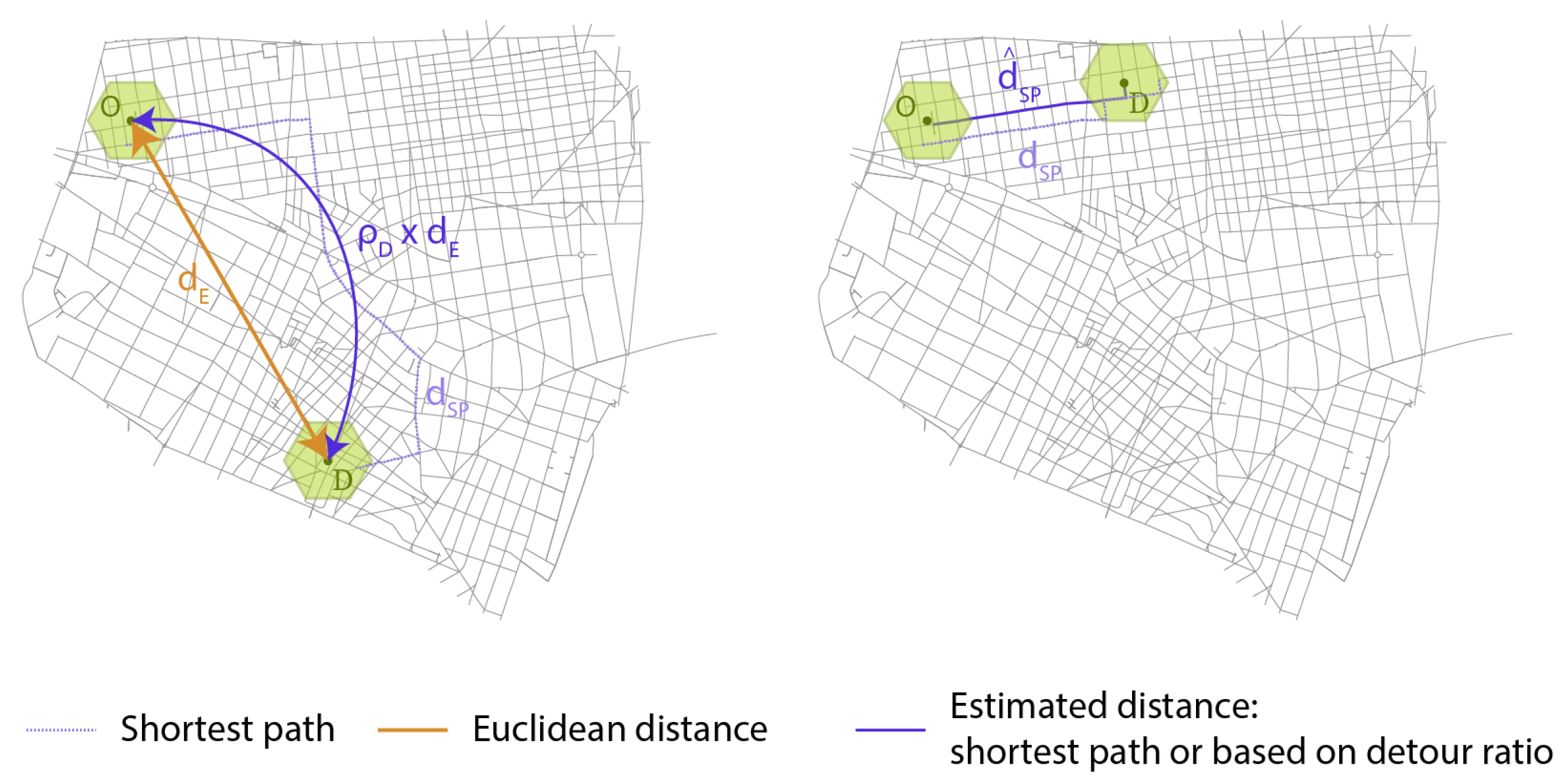
  • We develop a cost-efficient method to infer travelled distances based on origin and destination positions and detour ratio.
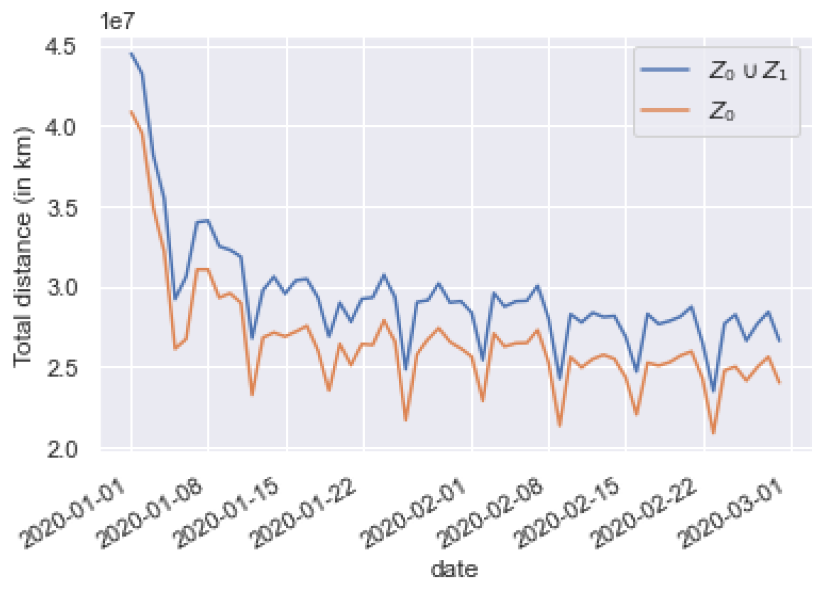
  • We test the method on two months of data covering the Colombian city of Santiago de Cali and evidence macroscopic patterns in the daily total travelled distances of nonregular travellers, including weekly seasonality and longer-term trends.
  • We additionally explore the macroscopic patterns of the overall population and draw research perspectives from the results.
The American communication provider CLARO provided the evaluation data to Citepa (a non-profit organisation and state operator for the French Environment Ministry) as part of a research and development project named Green City Big Data.
The rest of this article is structured as follows. Section 2 presents our methodology. Section 3 presents our case study and the available data. Section 4 displays the results of our method applied to that case study. Section 5 finally discusses the results and the improvement we consider as the following work.

2. Methodology

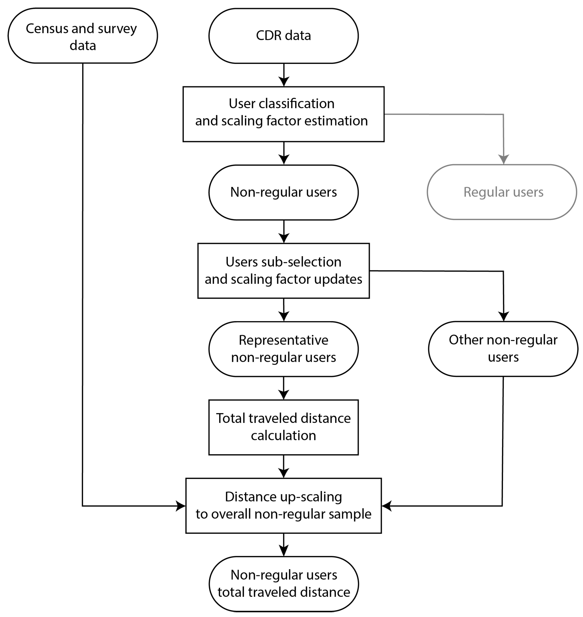
2.1. Design and Method Outline

We assume that travellers can be divided into two categories: regular and nonregular travellers. Considering an urban study area of limited extent, nonregular travellers include both occasional visitors and travellers that are frequently observed in the area but have non-recurrent activity chains. Therefore, a preliminary step of our work is to separate CDR users into such two classes (Section 2.2).
Then, reconstructing the mobility patterns of nonregular users raises the question of determining an analysis variable adapted to this population. Origin–destination matrices are the most frequent mobility variable estimated to represent mobility patterns based on the extraction of trips from mobile phone data. However, their upscaling to the overall population implicitly assumes that the sampled user activity chains are representative of the overall population. This assumption can be considered satisfactory when considering travellers moving regularly. However, when analysing nonregular travellers, it is not valid anymore; the global mobility of such users cannot be abstracted from observations made on a single day. This problem, often neglected in the literature, requires defining a larger scale of analysis and selecting mobility variables, such as distance travelled, appropriate for studying nonregular users.
To estimate those distances, one must overcome the bias that incomplete mobility data (as derived from CDRs) imply. To this end, we design a collective mobility reconstruction approach involving the definition of a data completeness attribute and the selection of representative nonregular users on that basis (Section 2.3). Then, we develop a method to estimate efficiently travelled distances from mobility data limited to origin and destination information (Section 2.4), well adapted to the scarce trajectory information characterising CDR data. The method relies on the concept of detour ratio, introduced in [18]. We apply it to the subsample of users whose communication activity provides reliable distance estimation, then upscale the results to represent the overall nonregular population. Figure 1 illustrates this overall process.

2.2. Nonregular Travellers Extraction

The first stage of our methodology involves identifying nonregular travellers from CDR data. Two successive classification methods are proposed to reach this objective.
The first classification step aims at categorising users according to their daily presence profile in the area. The main objective is to identify local users versus visitors. The literature proposes many different approaches to carry out rich classifications [19,20,21,22,23]. We adopt a binning approach based on the definition of some simple rules that allow us to separate the population into three subgroups: residents, commuters, and visitors. Macroscopic indicators derived from census and survey data helped calibrate the binning rules. This classification process is presented in Appendix A and further details of this approach can be found in [24]. Once users are classified, we can relate the sample sizes | s | (e.g., detected residents, commuters, or visitors) to the size of the corresponding groups | P s | within the overall population (respectively, overall population of residents, commuters, or visitors) to associate to each a scaling factor f s :
f s = | P s | | s |
The second classification step involves identifying nonregular users from residents and commuters (local users). Visitors are considered nonregulars by default. The classification of local users relies on the measurement of their temporal–uncorrelated entropy S u [25]:
S u = i = 1 N u p u ( i ) · l o g 2 p u ( i )
where p u ( i ) is the historical probability of user u visiting location i, i.e., the total number of times user u visited location i over the study period, divided by the total number of visits generated by u over the study period [25,26]. The users whose entropy is below one standard deviation above the mean value are considered regular travellers, others as nonregulars. In our case study, Santiago de Cali, this results in a classification of 11% of the local (residents and commuters) population as nonregular. At the same time, we estimate that nonregular users are slightly more represented in the commuter population (13%) than in the resident one.

2.3. Subsample Selection for Collective Mobility Reconstruction

The second stage of the method focuses on identifying a subsample of users with fully characterised mobility patterns.
Users’ sparse communication rates may prevent observing their mobility patterns to their full magnitude. Not detecting a trip or visit because of long interevent times can result in misunderstanding the user’s activity chain, trajectories, and overall travelled distance. The literature provides user-centric latent mobility reconstruction approaches [7,13] to tackle this issue, filling the mobility gaps with history-based automatic learning. These methods are adapted to regular users, but the little history or lack of redundancy of mobility patterns of nonregular users prevent using such a method. Therefore, a more collective mobility reconstruction approach is needed.
We make the following hypothesis. We assume that the distance travelled by users is independent of their communication rates. Under this hypothesis, the most active share of the population (whose mobility patterns can be considered complete) is considered statistically representative of the less communicating users.
We introduce metric ρ c to measure individual daily data completeness and suppose that we can identify a minimum threshold ρ c m i n above which the travel distances are well estimated.
Different completeness metrics can be defined. In [13], authors use “the fraction of time intervals [of one hour] for which [they] have at least one location sample”. Due to the specific features of the data used in this paper (cf. Section 3), we instead choose as a metric the daily time with known positioning. For a given user, let S be the set of sequences of consecutive communication events occurring at the same location, and let δ s be the duration of such a sequence s. We define daily completeness as:
ρ c = s S δ s Δ d
where Δ d is the duration of the day.
Note that when sequences are made of a single communication event, i.e., their duration is null, we disregard them from the completeness computation. In practice, the literature generally considers those nonlasting sequences as pass-by points of a trip, as opposed to the long sequences assimilated to static activities. Therefore, our approach bases the study of completeness on the static activities of users.
Thereafter, we will note U d i r r the set of irregular users observed on day d, and U d i r r , c the subset of irregular users observed on day d whose data completeness exceeds ρ c m i n :
U d i r r , c = { u U d i r r | u . ρ c > ρ c m i n }
On the contrary, let U d i r r , p be the set irregular users observed on day d that display partial mobility data. We propose to estimate the distance travelled by the subpopulation U d i r r , p before expanding the conclusions to the overall nonregular users U d i r r .

2.4. Travel Distance Calculation

2.4.1. Metric Definition

The distance calculation method we apply to users in U d i r r , c relies on an initial data processing phase to identify the different locations visited during the day by travellers. This topic is out of the scope of this paper, especially as the method applied is extracted from well-known literature addressing the issue [10,27]. The method consists of classifying communication events as either static or dynamic. Static events are aggregated into mobility phases called stays, whereas dynamic events characterise trajectories in between stays.
However, the burstiness of human communication patterns [6,28,29,30] and the spatial resolution of the data often result in trajectories too sparse for the direct estimation of distances travelled. Instead, we use the shortest path between consecutive static communication sessions as a proxy for the distance travelled. Depending on the network density and size, computing the shortest paths can be costly; we develop a lightweight hybrid approach which does not systematically rely on actual shortest path computation.
We adapt the concept of detour ratio, first introduced by [18] to nominate the ratio of the trip length d with a baseline distance d R , e.g., the Euclidean distance [3,18] or the shortest path distance [3]. This concept characterises the extra amount of distance travelled compared to the baseline distance. We adjust this notion by defining a detour ratio ρ D as the ratio of the shortest path distance d S P with the Euclidean d E :
ρ D = d S P d E
The detour ratio ρ D can be calibrated as a function of Euclidean distance d E using a limited set of synthetic shortest paths on the studied network. Then, given the Euclidean distance between two geographic positions p and q, one can estimate the shortest path distance as:
d ^ S P ( p , q ) = ρ D ( d E ( p , q ) ) · d E ( p , q )
This approach provides a cost-effective method to estimate the shortest path distance from one position to the other and is particularly fitted to large networks. Its main limitation is that the detour ratio presents a significant variability for short Euclidean distances, for which it should not be trusted. We overcome this issue with a dedicated approach to small Euclidean distances, for which we resort to a direct shortest path distance calculation. This calculation is facilitated by the analysis of a limited spatial perimeter, and therefore short computation times.
To summarise, we define a hybrid method d H to estimate the shortest path distance between two consecutive visited locations, based on direct shortest path identification for short Euclidean distances and on a cost-efficient shortest path distance approximation with detour ratio for larger Euclidean distances. Plotting the detour ratio function can provide a reasonable value for the distance threshold d m i n determining for which distance each of those two approaches should be used. The metric d H is formally defined below:
d H : R 2 × R 2 R ( p , q ) d H ( p , q ) = d S P ( o d ) if d E ( p , q ) < d m i n d H ( p , q ) = ρ D ( d E ( p , q ) ) · d E ( p , q ) if d E ( p , q ) d m i n
where d S P ( p , q ) is the shortest path distance between positions p and q. Figure 2 provides an illustration for each of these methods. The overall daily distance travelled by a user is simply defined as the sum of distances of the trips of the user’s activity chain A = ( a 0 , , a n ) :
T T D u = i n 1 d H ( a i , a i + 1 )

2.4.2. Validation

Using a detour ratio function to estimate shortest path distances necessarily results in approximation in the distance estimations. These errors can be additionally fuelled by the coarse spatial resolution of the communication network; estimating distances from one base station to the other necessarily implies a bias compared to the distance between the microscopic origin and destination points. We propose a simple validation framework to evaluate these errors.
First, we generate synthetic trips at the scale of the road network by sampling origin and destination nodes and computing the shortest path between them. Second, we degrade the origin and destination positions to the corresponding base stations ( b o , b d ) , to represent the information retrieved from mobile phone data. Using those estimated origin and destination positions, we compute both the Euclidean distance d E ( b o , b d ) and the hybrid distance d H ( b o , b d ) , and compare both of them to the reference shortest path distance. The results of this analysis are presented in Section 4.2.

2.5. Distance Upscaling
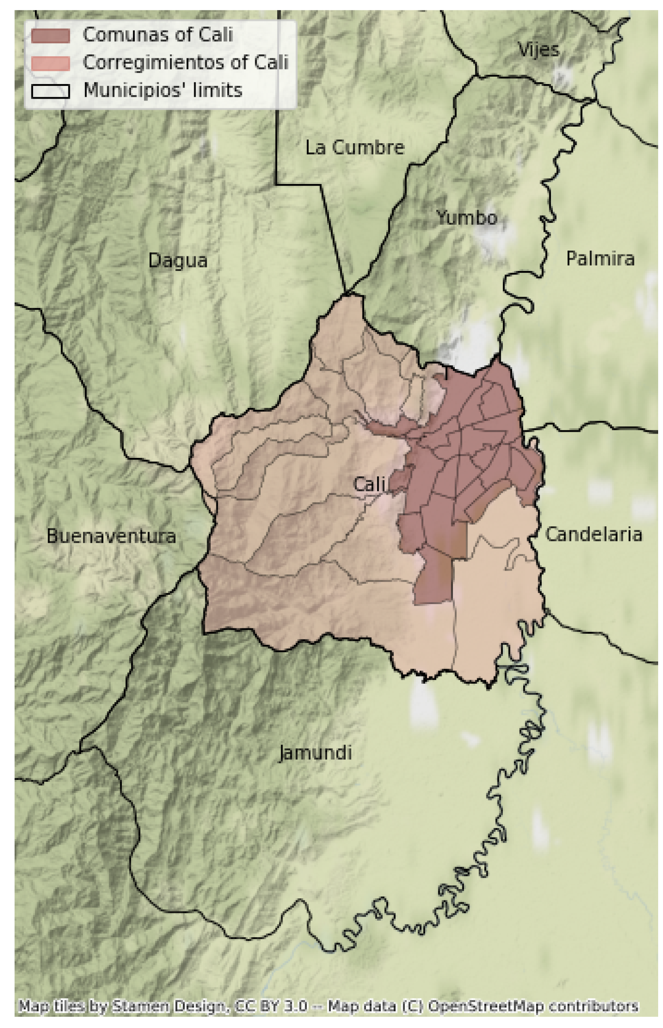
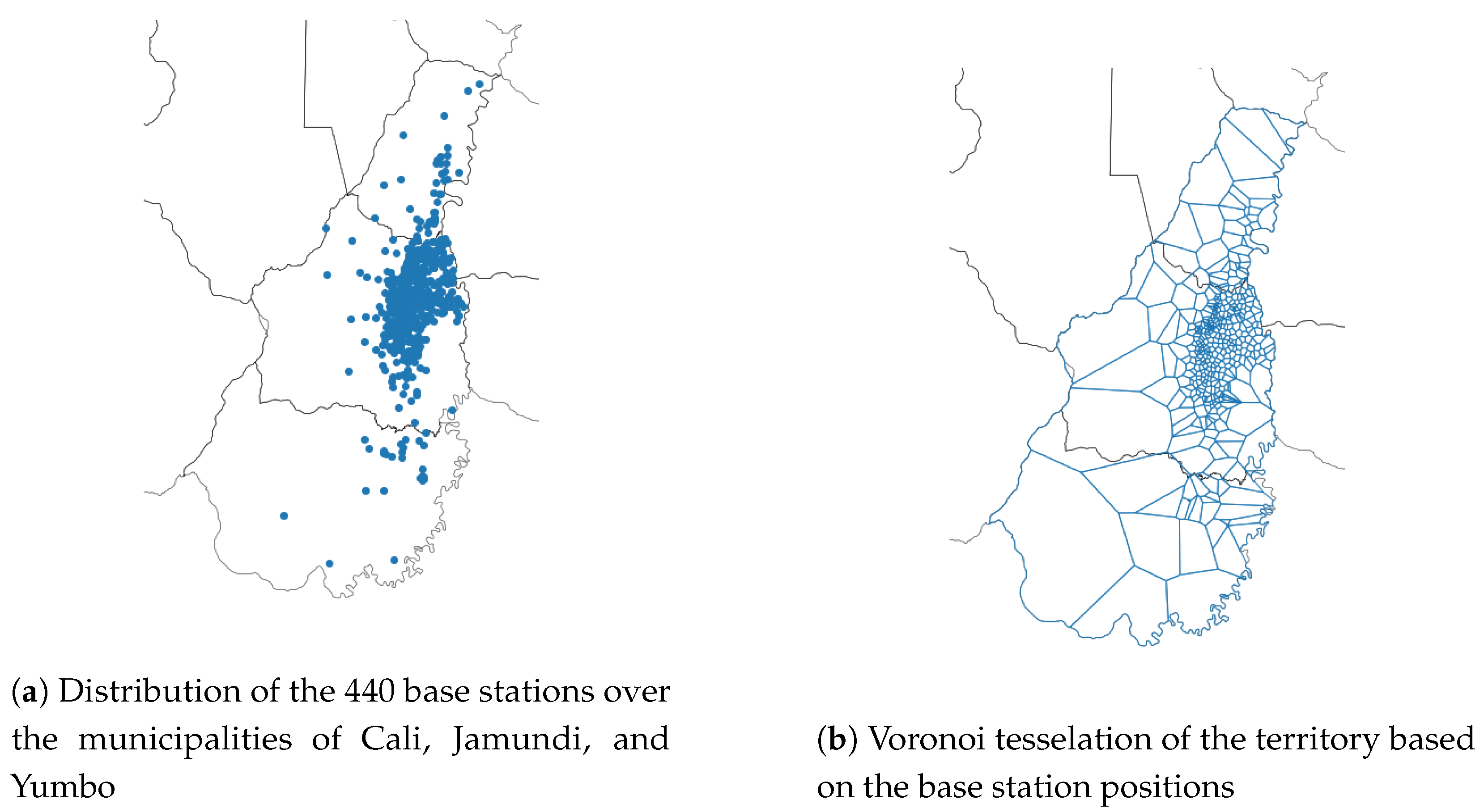
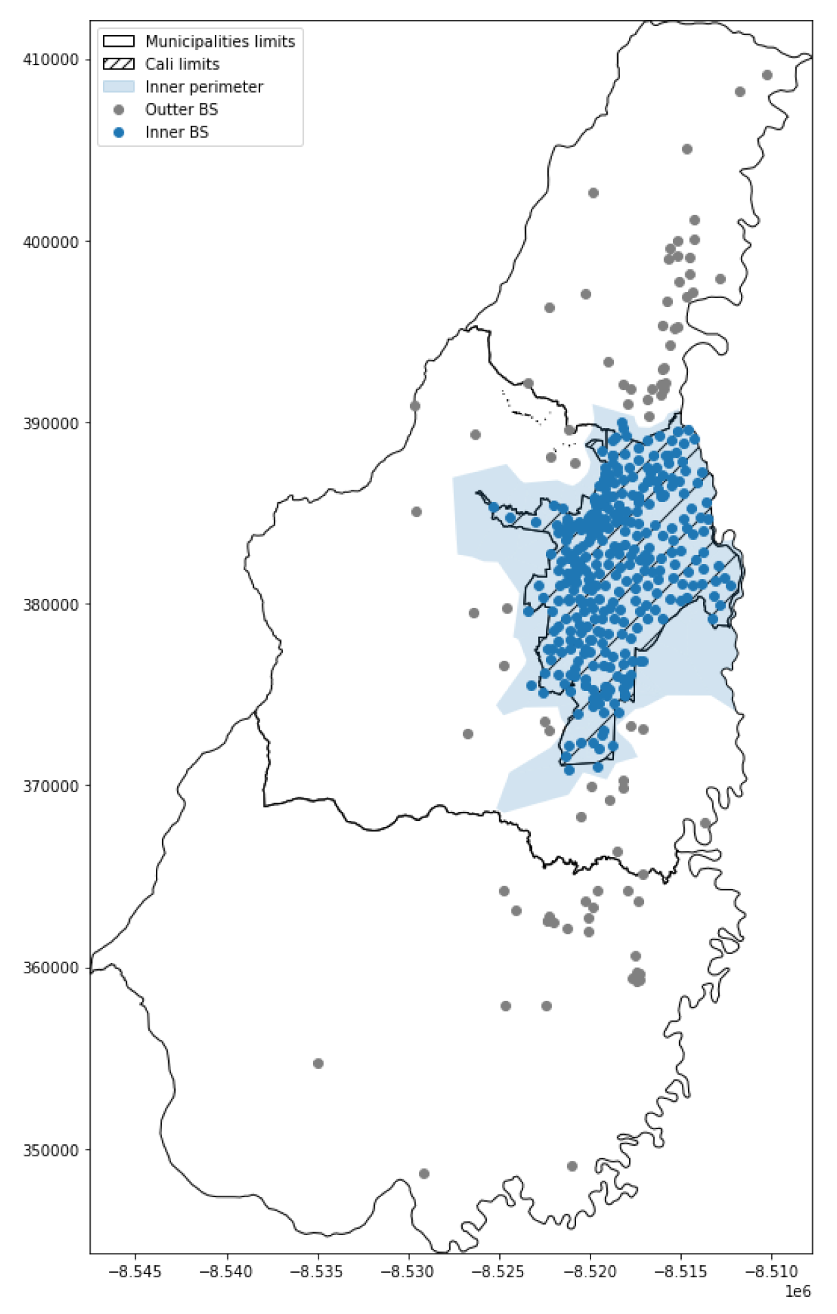
Once the daily travel distances of individuals in U d i r r , a have been estimated, we perform a double scaling to extrapolate the conclusions to the population it represents. First, the individual distances are upscaled according to the weight f u = f s of the sample s to which the user u belongs.
T T D i r r , a = u U d i r r , a T T D u f u
Then, the resulting total distance is further upscaled in order to represent as well the population that was filtered because of too little data completeness.
T T D i r r = T T D i r r , a · u U d i r r f u u U d i r r , a f u

3. Case Study

This methodology was applied to mobile phone data provided by the American communication provider CLARO to Citepa, the French state operator leading this research project. The data horizon length is two months of the pre-COVID-19 period (January and February 2020). Its spatial coverage consists of the greater area of the Colombian city of Santiago de Cali, the third most populous city in Colombia.
For privacy protection and transfer efficiency reasons, the data shared by CLARO was compressed and reduced to the mobility information only. Users’ consecutive communication events occurring at the same base station were aggregated into a unique communication sequence entry. The resulting communication sequences were characterised by the users id, the base station location, the timestamps of the first and last event of the sequence, and the number of events observed during the sequence. Table 1 and Table 2 provide an illustration of regular CDR data and the format of the data as shared by CLARO.
The shared data covers the 22 urban and 15 rural districts of Cali and two neighbouring municipalities, Yumbo in the north and Jamundi in the south (see Figure 3). Table 3 provides extensive population and surface indicators of the covered area.
A total number of 440 base stations are covering Cali, Yumbo, and Jamundi with an uneven density. The base station network is denser in the city centre than in the city surroundings, where approximately 70% of the base stations are located. The network density there is 2.79 base stations per square kilometre, whereas it is 0.16 base stations per square kilometre outside of Cali. Figure 4a illustrates the inhomogeneous distribution of the base stations over the area and Figure 4b represents the Voronoi’s tesselation of the base station network. This tesselation is classically used in the literature to represent the spatial resolution of the data. It identifies the theoretical geographical area covered by each base station. This tesselation is often used to infer the users’ positions by assuming that users’ events are processed by the closest base station.
In order to estimate the distance travelled both within the city and in its surrounding rural districts, we divide the base station network into two large subareas. As the tessellation defined by the Voronoi’s polygons of the BS network does not match the administrative boundaries of the city, we associate to the inner city of Cali all the base stations’ antennas located within a buffer of 700 metres outside of its administrative border. Note that since these base stations have variable spatial coverage, the resulting area boundary may be irregularly distant from the administrative city limits, as can be seen in Figure 5. Thereafter, we will call Z 0 the inner region and Z 1 the outer area.

4. Results

This section first presents three short methodological studies:
  • the calibration of the detour ratio function required to set up the parameters of d H ;
  • the evaluation of the approximations implied by d H ;
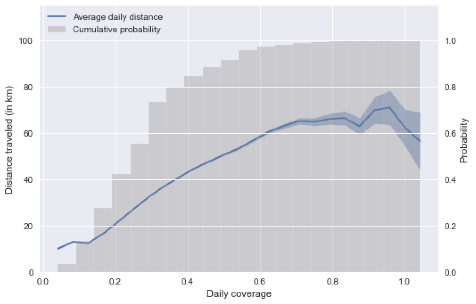
  • the determination of a reasonable individual data completeness threshold for selecting nonregular travellers used for mobility reconstruction.
Then, we conduct an extensive analysis of the mobility patterns over the two months of data.

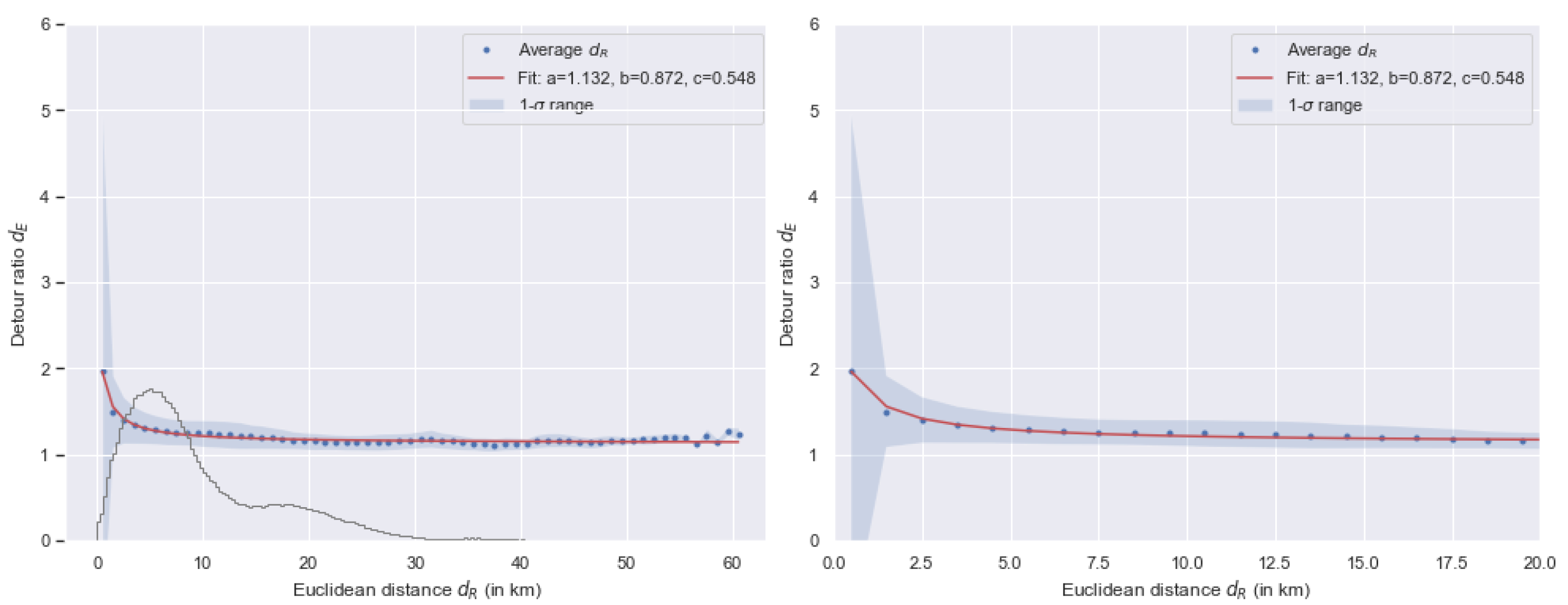
4.1. Detour Ratio Calibration

A set of synthetic origins and destinations are sampled from the network and used for calibrating the detour ratio function in Cali. For each trip, both the Euclidean and shortest path distance between the origin and the destination are measured. Applying Equation (5), we compute the corresponding detour ratio and relate it to the Euclidean distance. The detour ratio values are averaged by steps of 500 m, and those measurements are used to fit a decaying relationship describing ρ d as a function of d E , as illustrated in Figure 6. We found this curve can be fitted by:
ρ D = 1.132 + 0.872 d E + 0.548
with R 2 = 0.97 . This relationship provides the numerical values for estimating the shortest path distance directly from the Euclidean one.

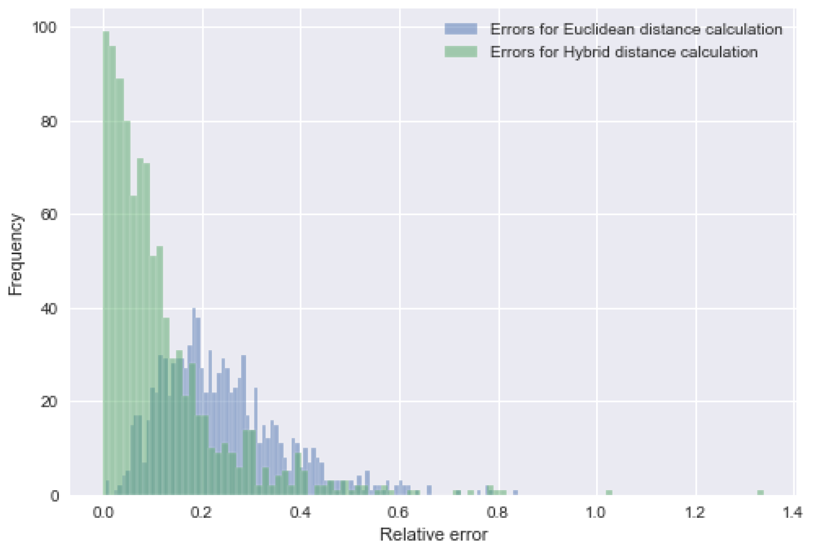
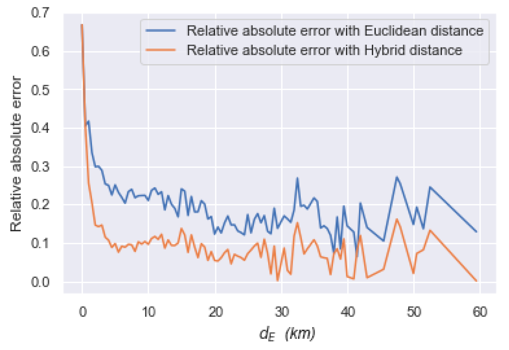
4.2. Hybrid Distance Metric Evaluation

In this section, we implement the evaluation protocol described in Section 2.4.2. The objective is twofold. First, it is a question of evaluating the estimation errors introduced by our method in comparison with the lengths actually travelled if travellers followed the shortest path. Secondly, it is also a question of identifying the gain compared to a simple calculation of distances based on Euclidean distances, used in some literature works.
Using 2000 synthetic trips on the city of Cali, we compare the real shortest path distance to the estimated distance using the hybrid metric d H and using the Euclidean distance d E instead. In both cases, we evaluate the absolute relative error. Figure 7 displays the distribution of these errors. The green distribution represents the error distribution for metric d H , whereas the blue one represents the error distribution for metric d E . The hybrid metric provides smaller errors than the Euclidean one, with most errors being bounded below 20%. In addition, we analyse the evolution of the average relative errors with the Euclidean distance. Results are presented in Figure 8. Since we are measuring relative errors, it is no surprise that the errors increase drastically when the Euclidean distance approaches 0. However, when d E increases, the average errors using the hybrid metric (orange line) quickly get bounded around 10%. This value oscillates around 20% for the Euclidean distance (blue line). The strong variability of the plot above a Euclidean distance of 30 km is explained by the limited sample of trips of such lengths.
On average, the deviation from the d S P distance is twice as small with the d H distance as with the Euclidean distance and remains contained around 10%.

4.3. Sensitivity Analysis

This section presents the analysis of the sensitivity of the individual distance estimate to the daily communication level.
We compute the daily data completeness ratio for a sample of 30,000 users and relate it to measured travelled distances. The objective is to determine if there is a data completeness threshold above which more communication information does not provide more mobility information. It is displayed in Figure 9 along with the cumulative distribution of the daily number of events. Up to a completeness of 0.6, we observe a linear growth of the average daily distance travelled with the daily number of events. After this completeness threshold, we observe a stabilisation of the average travel distance at a level of approximately 60 km. This stabilisation seems to confirm that beyond a certain completeness threshold, the estimated distances are well represented: more data does not mean more distance travelled. This 0.6 value is on a daily basis to set the completeness threshold ρ c m i n used to separate U d i r r , c and U d i r r , p . On a daily basis, U d i r r , c represents approximately 5% of U d i r r , which seems satisfactory to retrieve reliable statistics.

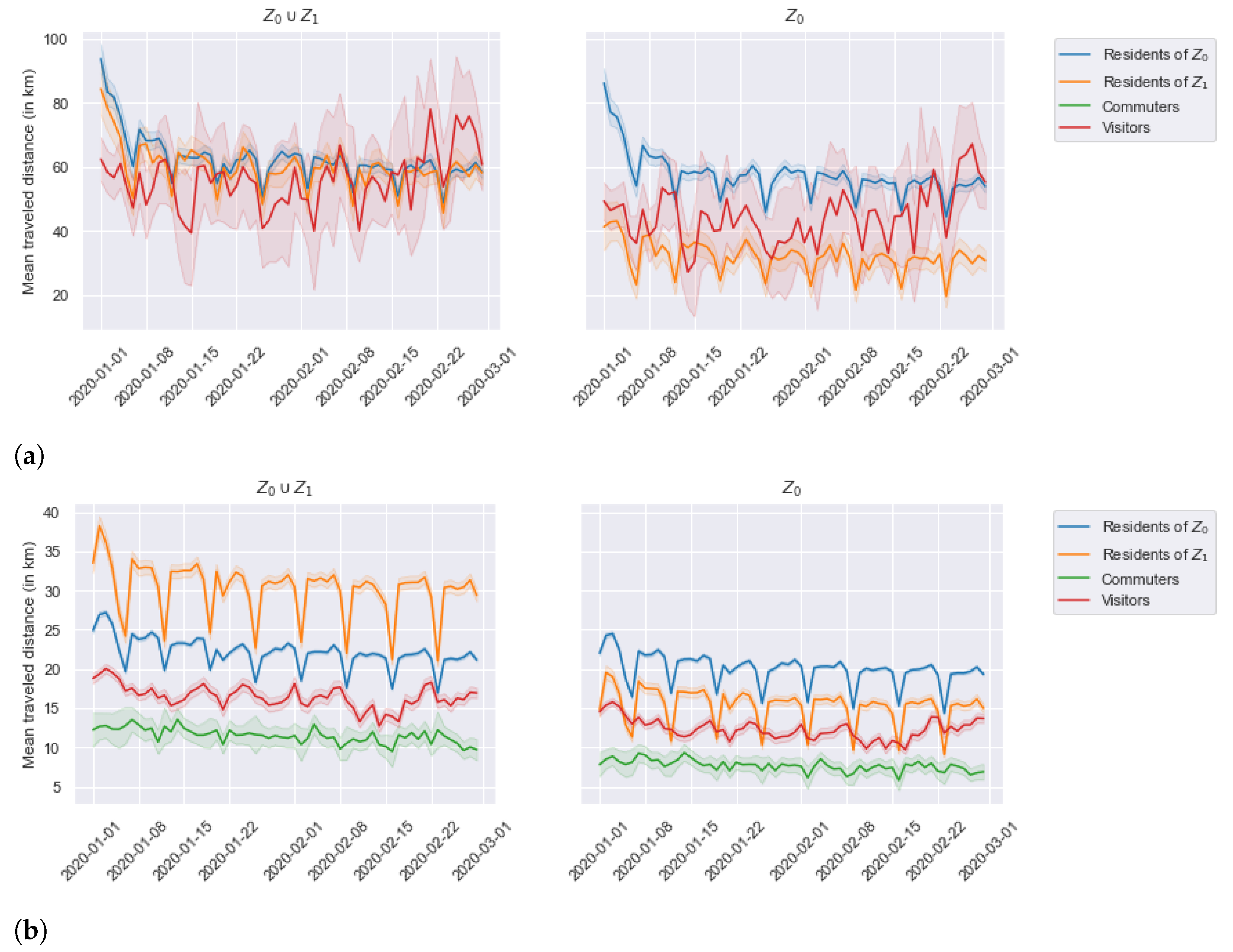
4.4. Application Analysis

In this section, we explore the results of the application of the detour ratio approach for estimated distances travelled by users. We first evaluate the total travel distances for the irregular population, then further investigate the distances travelled within the overall population for each different user category.
Figure 10 displays the total travel distances estimated for the irregular population U i r r , based on a estimation derived from users of U i r r , c and upscaled to the users of U i r r , p . The blue line represents the trend in the overall region Z 0 Z 1 , whereas the orange line represents the distance travelled within the city of Cali only ( Z 0 ). To allocate the distance travelled to the city centre ( Z 0 ) or the rural areas ( Z 1 ), we draw a straight line from the origin to the destination and simply evaluate in which proportion it intersects Z 0 or Z 1 . The distance allocation is distributed accordingly. It appears that the city of Cali represents a very significant share of the distances travelled in the agglomeration.
We observe clear weekly seasonality effects with distance drops on Sundays, coupled with a notable increase in the distance travelled at the beginning of the study period, which corresponds to the New Year celebrations and vacations. This increase can be explained by two factors: first, a probable influx of individuals considered irregular, the visitors; second, a possible increase in the average distance travelled by users during this holiday period. The number of kilometres travelled is significant. When compared to the total distance travelled, we estimate that irregular users contribute to 19 to 25% of the mobility volume.
Figure 11 illustrates this trend. Interestingly, it shows how the irregular users have an increased weight in the global mobility on a weekly basis as well. This weight rises every Sunday, which means that even though irregular users are relatively less mobile on Sundays, their mobility drop is weaker than for the regular users. Together, these plots show that irregular users contribute to an important share of the total travelled distance and therefore that they should not be neglected.
In Figure 12, the total travelled distances of the overall population is displayed, separated by presence profile (residents of Z 0 and of Z 1 , external commuters, and visitors), as identified using the binning classification. Here again, the visualisation of the total travel distance plays a weekly regularity. We observe the significant difference of magnitude between the total travelled distance by residents and other user categories. This observation can question the utility of considering the contributions of those trajectories to the distance travelled. However, a deeper investigation showed that commuters and visitors travelled close to 300,000 km on a daily basis in the overall metropolitan area of Cali, which is considerable.
Furthermore, we note a significant impact of the completeness filter on commuters, drastically reducing the sample size. This is explained by the fact that commuting users live outside of the study area, and hence almost never spend more than 60% of their daily time in the study area. Therefore, the completeness ratio as it is defined in the paper is not adapted to this share of the population. This is an important limitation that should be addressed in future improvements of the method.
To compare patterns on a similar scale, we plot with Figure 13 the total travel distance of the overall population normalised by the maximal daily distance of the category. We propose two versions of this graph, the first one in the standard case where the population is reduced to the users with a completeness higher than 0.6 (Figure 13a), the second one based on all the users, whatever their completeness level (Figure 13b). This distinction demonstrates that although commuters are poorly represented in the population reduced to the most complete users, they actually have aggregate mobility patterns as regular as the other categories of the population. In Figure 13b, we clearly observe the temporal shift between the profiles of the most regular users (residents and commuters) and the profiles of the visitors. In the version reduced to a subsample of the population (Figure 13a), the temporal regularities appear less clearly. Due to smaller sample sizes and less robust expansion processes, the results are more sensitive to individual variations. The integration of larger amounts of data should limit the noise observed on the curves.
Figure 14 displays, for the overall user population, the average distance travelled by users for each considered mobility profile, both in the overall studied perimeter ( Z 0 Z 1 ) and in the inner city ( Z 0 ), and the 95% confidence interval. Figure 14a represents results derived from the analysis of patterns of users with complete mobility upscaled to the remaining population. In comparison, Figure 14b represents results derived from the direct distance estimation of the whole population. We make several observations.
First, the two estimation approaches return different magnitudes for the travelled distances. The application of our methodology (Figure 14a) provides higher travelled distances than with a direct estimation from all nonregular users (Figure 14b). On average, at the Z 0 Z 1 scale, the daily travelled distances vary between 40 and 60 km per day if we consider the estimates based on a restricted sample, against 15 to 35 with direct estimation. Two factors explain this difference. On the one hand, the mobility of users from U i r r , p is likely partial, which contributes to underestimating the actual travelled distance in Figure 14b. On the other hand, contrary to the hypothesis that we have made, the mobility of users from U i r r , c may not be entirely representative of the actual mobility of U i r r , p , and a correlation may exist between the communication activities and the mobility of individuals.
Due to the lack of ground truth data, validating these orders of magnitude is challenging. The surveys conducted by the administration of Santiago de Cali focus more on the travel time than on the trip distances [31]. In a paper whose analysis may be out of date [32], the authors approximated the total distance travelled per type of vehicle (e.g., cars or buses). Assigning a transportation mode to users or trips is out of the scope of this work; therefore, comparing our results to this kind of reference is not straightforward. However, we use the results of similar works, albeit more recent and conducted in countries other than Colombia, to put our orders of magnitude into perspective. For example, Chinese drivers have recently been reported to travel an average of 28 km per day [33], French drivers 33 [34], and Americans 59 [35]. In comparison, our results indicate that Cali residents travel on average between 20 km (without selection of users with complete data) and 60 km per day (with selection). These figures confirm the above hypothesis that the mobility estimated from unfiltered data is underestimated but that the drastic user selection is likely to also result in overestimation. However, one can consider those results as an upper bound of the distance travelled, which we will refine in future works. We discuss how in the conclusions.
Second, we observe that the study scale influences the relative contribution of different user categories. With the restricted sample analysis (Figure 14a), residents from Z 0 and Z 1 are observed to travel equivalent distances (60 km on average) at the scale of Z 0 Z 1 . At the scale of Z 0 instead, the two resident categories display different contributions: residents of Z 0 travel similar distances, whereas residents of Z 1 travel less than 40 km on average. This suggests that the residents from Cali’s surroundings ( Z 1 ) tend to travel more in that area than residents of Cali city centre. Interestingly, when not restricting the analysis to complete activity chains (Figure 14b), the results provide a slightly different point of view regarding this contribution to the distances travelled in Z 0 Z 1 . Residents from Z 1 are estimated to travel more kilometres on average (above 30) than residents from Z 0 (around 25). This difference compared to Figure 14a shows the sensitivity of the analysis to the filters we set on communication level and suggests different communication properties between users of Z 0 and Z 1 . At the scale of Z 0 however, we observe relative contributions comparable to those of Figure 14a.
Lastly, the comparative analysis of Figure 14a,b illustrates the impact of the completeness filter on sample sizes and statistical representativity both for commuter and visitor categories, as Figure 14a displays high variability and large confidence intervals. Daily visitors may present similar presence patterns to commuters and suffer from the too-high 0.6 completeness threshold.

5. Conclusions

This paper addresses the question of characterising urban mobility patterns from sparse mobile phone data (CDR) for nonregular travellers. The mobility of those travellers is not easy to analyse because of several issues. In addition to suffering from the general limitations of CDR data (coarse spatial resolution and variable sampling rates), the historical mobility data of these users are not regular enough to reconstruct the missing mobility information at an individual level. Furthermore, origin–destination matrices, traditionally used to represent mobility patterns, are inappropriate for representing the mobility of nonregular users because their activity chains cannot be considered representative.
We propose to evaluate mobility patterns through the scope of the total travel distances. We propose a collective mobility reconstruction approach: a subsample of nonregular travellers (with mobility chains weakly impacted by the mobile phone data sparsity) supports estimating the distances travelled by the whole group. The sample is selected according to a completeness threshold following a sensitivity analysis. The distance travelled by those users is estimated based on a hybrid distance estimation method. We consider that the shortest path distance is a reliable approximation of the distance travelled by the users, but avoid the costly computation of those shortest paths by designing a method relying on the concept of detour ratio. The detour ratio considered here compares the shortest path distance to the Euclidean distance. We show that this method generates limited errors in estimating the shortest path distance.
We apply our method to compressed call detail records provided by the American provider CLARO for Santiago de Cali, Colombia. The method is first applied only to nonregular users. This analysis evidences that nonregular users often dismissed from mobility analysis contribute to regular weekly macroscopic patterns of significant magnitude. Those results justify including such users more systematically in urban mobility analyses and suggest macroscopic approaches can better cope with those travellers than user-centric approaches.
We also explore the macroscopic mobility patterns of the overall population, classified according to different mobility profiles (residents, commuters, and visitors). This extensive analysis allows for identifying the critical limits of our method: the completeness threshold selected appears to be restrictive for commuters, and to some extent to visitors. As they live outside the study area, those users generally spend too little time within the area to reach the selected threshold. Therefore, the samples of “complete” users selected are too limited to provide representative mobility patterns. A solution to this issue will be defining a specific completeness threshold for each presence profile.
As often when processing mobile phone data, a challenging aspect of this study is the validation of the method outcomes. Our longitudinal analysis provides convincing results: increased weight of nonregular mobility on weekends, weekly seasonality of travelled distances, or impact on the mobility of events such as holidays. The lack of appropriate ground truth data prevents accurate validation of the numerical values. However, their comparison with some literature works on different study areas evidenced consistent orders of magnitude while suggesting a slight overestimation of our results. The hypothesis we make in this work, which assumes that individuals’ communication and mobility activities are independent, is likely to be responsible for this overestimation, as there might be a positive correlation between those two variables [36]. Characterising this relation will allow us to calibrate and apply correction factors to rectify this bias and refine our estimates. Besides, ongoing works for identifying modal share should allow us to estimate travel distances per mode and relate our analysis to some more ground truth statistics.
This latter research direction is also promising as it opens the door to other assessment perspectives, such as estimating air emissions from road traffic. In this direction, a key step will be to couple our collective nonregular mobility reconstruction approach with finer user-centric methods within a global, multiscale pattern evaluation framework.

Author Contributions

Conceptualization, M.S., L.L. and A.F.; methodology, M.S., L.L. and A.F.; software, M.S.; validation, M.S., L.L. and A.F.; data curation, T.V.d.R., J.-M.A. and J.B.; writing—original draft preparation, M.S.; writing—review and editing, M.S., L.L., A.F., T.V.d.R., J.-M.A. and J.B.; visualization, M.S.; supervision, L.L., A.F. and T.V.d.R.; project administration, T.V.d.R., J.-M.A. and J.B.; funding acquisition, T.V.d.R., J.-M.A. and J.B. All authors have read and agreed to the published version of the manuscript.

Funding

This research was funded by Citepa (French state operator on behalf of the French Ministry of the Environment) through a Cifre (French Industrial Agreements for Training through Research) contract (grant number 2018/0626).

Institutional Review Board Statement

Not applicable.

Informed Consent Statement

Not applicable.

Data Availability Statement

Restrictions apply to the availability of these data. Data was obtained through an industrial partnership with Claro, Bogota, Colombia and are not available for sharing.

Acknowledgments

This research was initiated by Citepa. It was carried out jointly by Citepa and the LICIT-ECO7 laboratory as part of a larger research project conducted by Citepa, named Green City Big Data. This research project is supported by a partnership with the Colombian data operator CLARO, which provided the mobile phone data.

Conflicts of Interest

The authors declare no conflict of interest.

Appendix A

Here, we present the main elements of the users classification according to their presence profile in Santiago de Cali and its greater area. The different classes targeted are defined as follows.
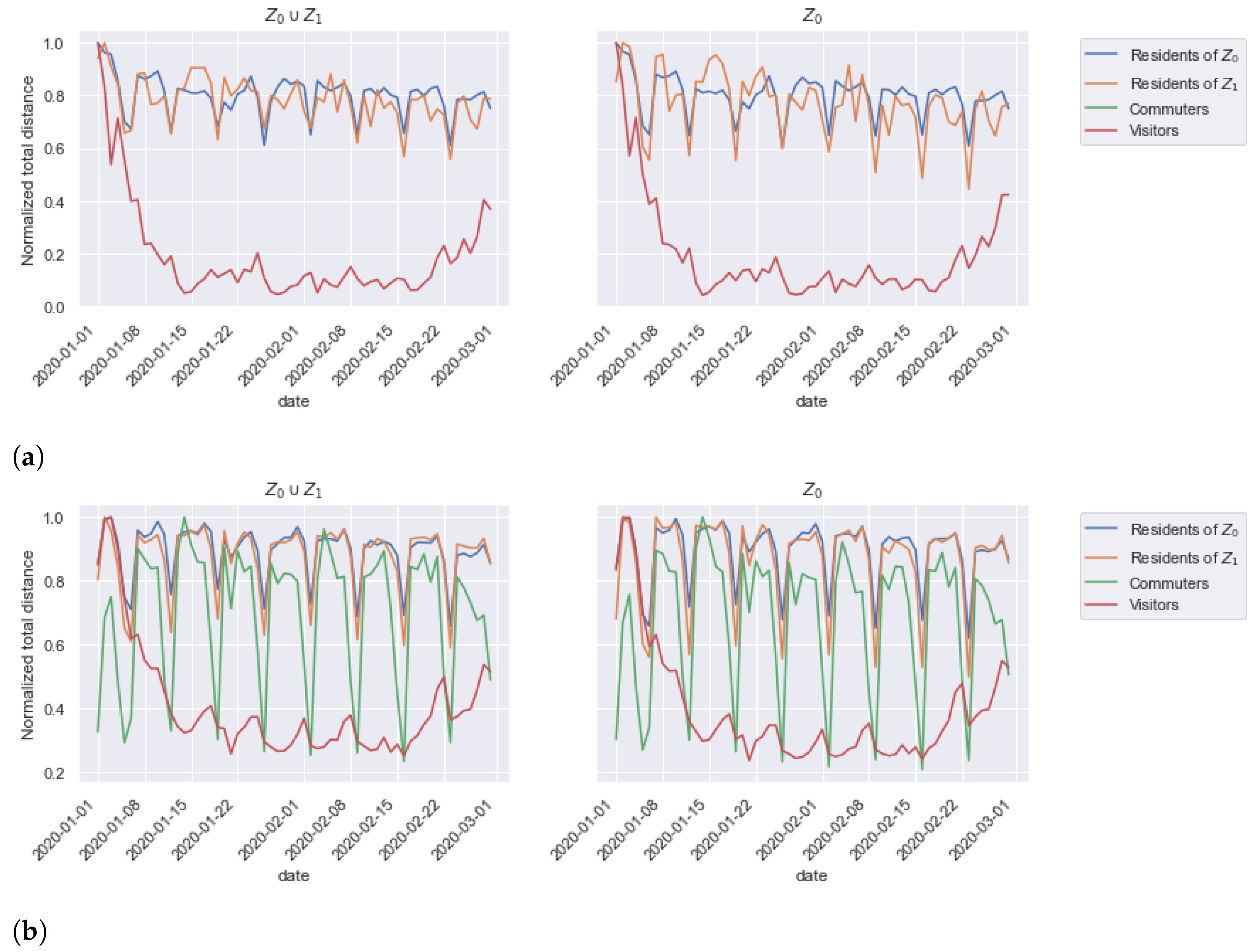
  • Residents R: individuals living in the area covered by the antennas;
  • Commuters C: individuals that live outside of the area but enter it on a frequent basis;
  • Visitors V: individuals that mainly live and work outside of the area, but may visit the studied territory, either for touristic reasons with a dense stay, or from time to time with shorter stays.

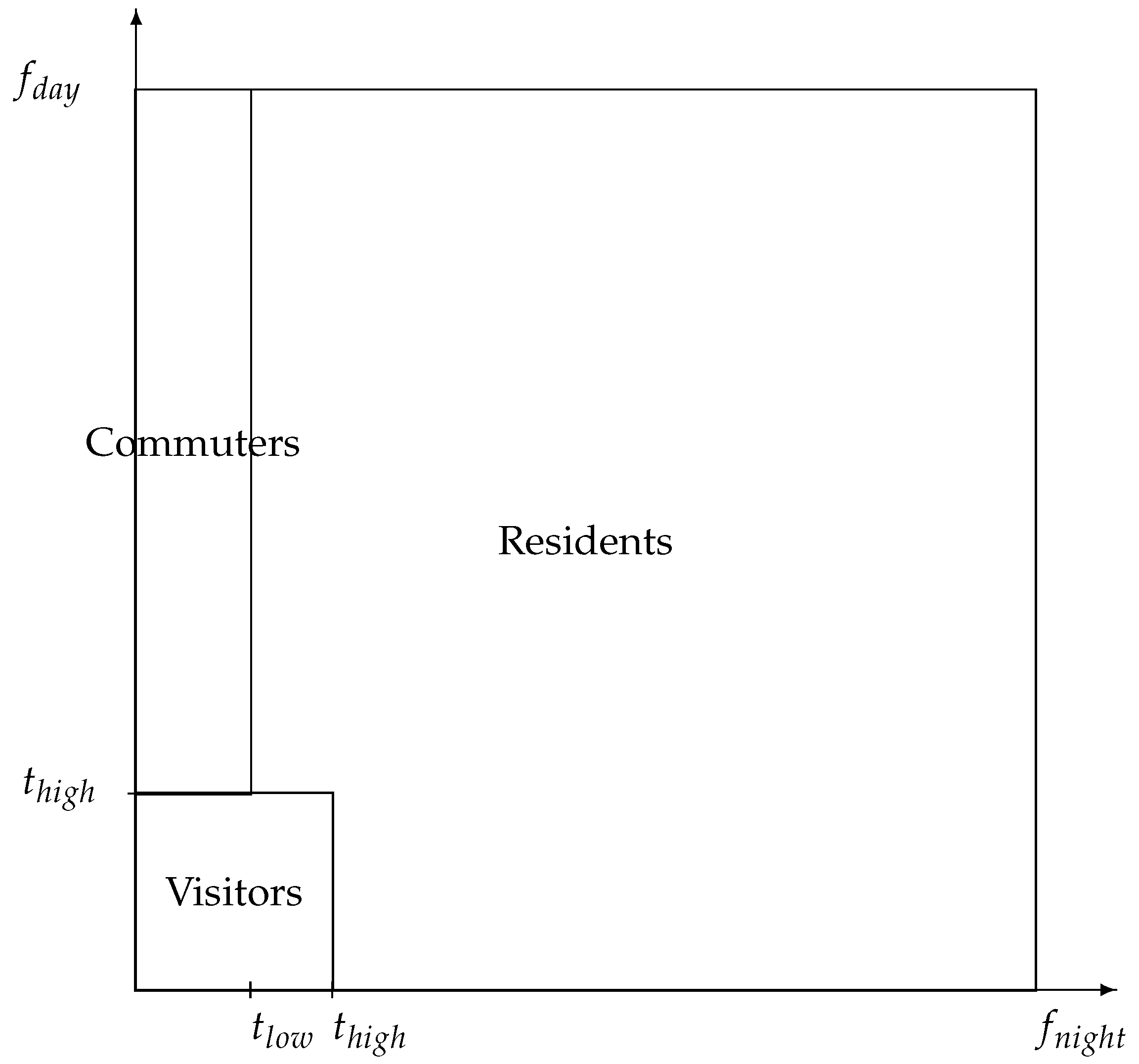
Appendix A.1. A Binning Approach

We use a simple binning approach, where the limits of the clusters are calibrated based on our observations of the individual behaviors. Based on the definitions selected previously, we consider as significant discriminating features the following ones:
  • f d a y : the number of days of observation in the area;
  • f w e e k D a y : the number of weekdays of observation in the area;
  • f n i g h t : the number of nights with observation in the area;
  • f m a x S t a y : the shortest stay (in number of consecutive days) observed over the historical period.
The parameters f d a y and f w e e k D a y isolate local users (residents and commuters) from visitors, whereas f n i g h t separates within local users the commuters from the residents. Introducing f m a x S t a y allows enriching the distinction between residents and commuters, commuters being expected not to appear in the area for too many consecutive days because of weekends. We partition the day into four time windows: night (8p.m.–7a.m.), early morning (7a.m.–9a.m.), restricted day (9a.m.–6p.m.), and late afternoon (6p.m.–8p.m.). Daily and nightly features are extracted from the night and the restricted day periods only, considering that the activities during early morning and late afternoon can vary from one day to the other.
We make explicit a set of binning rules, summarised in Table A1. Those rules rely on only two threshold parameters, t h i g h and t l o w . The threshold t h i g h aims at setting a high presence threshold that guarantees the users meeting these criteria are local users: they are present enough in the area, at night or day, to be considered either residents or commuters. The proposal of threshold t l o w is to extend the resident category to users who are sufficiently observed at day to be considered locals, and sufficiently observed at night to be considered residents instead of commuters.
Table A1. Binning rules.
Binning Rules Role
f n i g h t > t h i g h Present at night
Residentsor f n i g h t > t l o w and f d a y > t h i g h orpresent at day (w/ softer night condition)
or f m a x S t a y > t h i g h orhas at least a long stay
Commuters f w e e k D a y > t h i g h Present at day
and not a resident
Visitors User is not a resident Other users
nor a commuter.
Figure A1. User classification diagram in the ( f n i g h t , f d a y ) plan.
Futuretransp 03 00015 g0a1

Appendix A.2. Threshold Calibration

Let R 0 r e f and R 1 r e f be, respectively, the population of residents of the city of Cali ( Z 0 ) and of its greater area ( Z 1 ). Let also C 1 0 r e f be the populations of residents of Z 1 that commute to work in Z 0 . We assume that:
  • the penetration rates of the mobile technology within R 0 r e f and R 1 r e f are identical;
  • the penetration rates of the mobile technology within C 1 0 r e f and R 1 r e f are identical.
Note that these assumptions may not hold at a fine geographic scale or when comparing two different regions or differently urbanized areas, due to socio-economic characteristics. However, the geographic consistency and the aggregated spatial scale considered here support these assumptions in our case.
They allow us to define two macroscopic constants r 1 r e f and r 2 r e f (derived from census data [37] and local mobility survey [38]) that the groups of classified CDR data users should respect:
r 1 r e f = | R 1 r e f | | R 0 r e f | = 12 %
r 2 r e f = | C 1 0 r e f | | R 1 r e f | = 33 %
The ratio r 1 r e f describes the relation between the suburban and city population sizes, whereas ratio r 2 r e f characterizes the share of the suburban population that commutes to the city. We calibrate the thresholds t l o w and t h i g h so that the corresponding sampled population groups R 0 , R 1 , and C 1 0 respect those ratios. This is conducted with a systematic exploration of the ( t l o w , t h i g h ) plan, which results in setting t h i g h to 11 and t l o w to 7.
In this work, the resident and commuter classes are aggregated under the local users class. We look into their mobility regularity to identify regular and nonregular users, whereas visitor users are by default considered nonregular.

References

  1. Toch, E.; Lerner, B.; Ben-Zion, E.; Ben-Gal, I. Analyzing large-scale human mobility data: A survey of machine learning methods and applications. Knowl. Inf. Syst. 2018, 58, 501–523. [Google Scholar] [CrossRef]
  2. Bonnetain, L.; Furno, A.; El Faouzi, N.E.; Fiore, M.; Stanica, R.; Smoreda, Z.; Ziemlicki, C. TRANSIT: Fine-grained human mobility trajectory inference at scale with mobile network signaling data. Transp. Res. Part C Emerg. Technol. 2021, 130, 103257. [Google Scholar] [CrossRef]
  3. Paipuri, M.; Xu, Y.; González, M.C.; Leclercq, L. Estimating MFDs, trip lengths and path flow distributions in a multi-region setting using mobile phone data. Transp. Res. Part C Emerg. Technol. 2020, 118, 102709. [Google Scholar] [CrossRef]
  4. Seppecher, M.; Leclercq, L.; Furno, A.; Lejri, D.; Vieira da Rocha, T. Estimation of urban zonal speed dynamics from user-activity-dependent positioning data and regional paths. Transp. Res. Part C Emerg. Technol. 2021, 129, 103183. [Google Scholar] [CrossRef]
  5. Hoteit, S.; Chen, G.; Viana, A.C.; Fiore, M.C. Spatio-Temporal Completion of Call Detail Records for Human Mobility Analysis. In Proceedings of the Rencontres Francophones sur la Conception de Protocoles, l’Évaluation de Performance et l’Expérimentation des Réseaux de Communication, Quiberon, France, 29 May–2 June 2017. [Google Scholar]
  6. Chen, G.; Hoteit, S.; Carneiro Viana, A.; Fiore, M.; Sarraute, C. Enriching sparse mobility information in Call Detail Records. Comput. Commun. 2018, 122, 44–58. [Google Scholar] [CrossRef] [Green Version]
  7. Zhao, Z.; Koutsopoulos, H.N.; Zhao, J. Identifying Hidden Visits from Sparse Call Detail Record Data. Trans. Urban Data Sci. Technol. 2021, 1, 121–141. [Google Scholar] [CrossRef]
  8. Iqbal, M.S.; Choudhury, C.F.; Wang, P.; González, M.C. Development of origin–destination matrices using mobile phone call data. Transp. Res. Part C Emerg. Technol. 2014, 40, 63–74. [Google Scholar] [CrossRef] [Green Version]
  9. Alexander, L.; Jiang, S.; Murga, M.; González, M.C. Origin–destination trips by purpose and time of day inferred from mobile phone data. Transp. Res. Part C Emerg. Technol. 2015, 58, 240–250. [Google Scholar] [CrossRef]
  10. Toole, J.L.; Çolak, S.; Sturt, B.; Alexander, L.P.; Evsukoff, A.; González, M.C. The path most traveled: Travel demand estimation using big data resources. Transp. Res. Part C Emerg. Technol. 2015, 58, 162–177. [Google Scholar] [CrossRef]
  11. Nanni, M.; Trasarti, R.; Furletti, B.; Gabrielli, L.; Van Der Mede, P.; De Bruijn, J.; De Romph, E.; Bruil, G. Transportation Planning Based on GSM Traces: A Case Study on Ivory Coast. In Proceedings of the Citizen in Sensor Networks, Barcelona, Spain, 19 September 2013; Nin, J., Villatoro, D., Eds.; Springer International Publishing: Cham, Switzerland, 2014; pp. 15–25. [Google Scholar]
  12. Çolak, S.; Alexander, L.P.; Alvim, B.G.; Mehndiratta, S.R.; González, M.C. Analyzing cell phone location data for urban travel: Current methods, limitations, and opportunities. Transp. Res. Rec. J. Transp. Res. Board 2015, 2526, 126–135. [Google Scholar] [CrossRef]
  13. Chen, G.; Viana, A.C.; Fiore, M.; Sarraute, C. Complete trajectory reconstruction from sparse mobile phone data. EPJ Data Sci. 2019, 8, 30. [Google Scholar] [CrossRef]
  14. Nilbe, K.; Ahas, R.; Silm, S. Evaluating the Travel Distances of Events Visitors and Regular Visitors Using Mobile Positioning Data: The Case of Estonia. J. Urban Technol. 2014, 21, 91–107. [Google Scholar] [CrossRef]
  15. Sikder, R.; Uddin, M.J.; Halder, S. An efficient approach of identifying tourist by call detail record analysis. In Proceedings of the 2016 International Workshop on Computational Intelligence (IWCI), Dhaka, Bangladesh, 12–13 December 2016; pp. 136–141. [Google Scholar] [CrossRef]
  16. Arai, A.; Fan, Z.; Matekenya, D.; Shibasaki, R. Comparative Perspective of Human Behavior Patterns to Uncover Ownership Bias among Mobile Phone Users. ISPRS Int. J. Geo-Inf. 2016, 5, 85. [Google Scholar] [CrossRef] [Green Version]
  17. Arai, A.; Witayangkurn, A.; Kanasugi, H.; Fan, Z.; Ohira, W.; Cumbane, S.; Miyazawa, S.; Ranjit, S.; Batran, M.; Shibasaki, R. Building a Data Ecosystem for Using Telecom Data to Inform the COVID-19 Response Efforts; Zenodo: Geneva, Switzerland, 2020. [Google Scholar] [CrossRef]
  18. Yang, H.; Ke, J.; Ye, J. A universal distribution law of network detour ratios. Transp. Res. Part C Emerg. Technol. 2018, 96, 22–37. [Google Scholar] [CrossRef]
  19. Furletti, B.; Gabrielli, L.; Renso, C.; Rinzivillo, S. Identifying Users Profiles from Mobile Calls Habits. In Proceedings of the ACM SIGKDD International Workshop on Urban Computing, Beijing, China, 12 August 2012; ACM: New York, NY, USA, 2012; pp. 17–24. [Google Scholar] [CrossRef]
  20. Furletti, B.; Gabrielli, L.; Renso, C.; Rinzivillo, S. Analysis of GSM calls data for understanding user mobility behavior. In Proceedings of the 2013 IEEE International Conference on Big Data, Santa Clara, CA, USA, 6–9 October 2013; pp. 550–555. [Google Scholar] [CrossRef]
  21. Gabrielli, L.; Furletti, B.; Trasarti, R.; Giannotti, F.; Pedreschi, D. City users’ classification with mobile phone data. In Proceedings of the 2015 IEEE International Conference on Big Data (Big Data), Santa Clara, CA, USA, 29 October–1 November 2015; pp. 1007–1012. [Google Scholar] [CrossRef]
  22. Mamei, M.; Colonna, M. Analysis of tourist classification from cellular network data. J. Locat. Based Serv. 2018, 12, 19–39. [Google Scholar] [CrossRef]
  23. Thuillier, E.; Moalic, L.; Lamrous, S.A.; Caminada, A. Clustering Weekly Patterns of Human Mobility Through Mobile Phone Data. IEEE Trans. Mob. Comput. 2018, 17, 817–830. [Google Scholar] [CrossRef] [Green Version]
  24. Seppecher, M. Mining Call Detail Records to Reconstruct Global Urban Mobility Patterns for Large Scale Emissions Calculation. Ph.D. Thesis, ENTPE, Univ. Gustave Eiffel, Univ. Lyon, Citepa, Paris, France, 2022. [Google Scholar]
  25. Song, C.; Qu, Z.; Blumm, N.; Barabasi, A.L. Limits of Predictability in Human Mobility. Science 2010, 327, 1018–1021. [Google Scholar] [CrossRef] [Green Version]
  26. Lin, Z.; Lyu, S.; Cao, H.; Xu, F.; Wei, Y.; Samet, H.; Li, Y. HealthWalks: Sensing Fine-Grained Individual Health Condition via Mobility Data. Proc. ACM Interact. Mob. Wearable Ubiquitous Technol. 2020, 4, 1–26. [Google Scholar] [CrossRef]
  27. Jiang, S.; Fiore, G.A.; Yang, Y.; Ferreira, J.; Frazzoli, E.; González, M.C. A review of urban computing for mobile phone traces: Current methods, challenges and opportunities. In Proceedings of the UrbComp@KDD, Chicago, IL, USA, 11 August 2013. [Google Scholar]
  28. Candia, J.; González, M.C.; Wang, P.; Schoenharl, T.; Madey, G.; Barabási, A.L. Uncovering individual and collective human dynamics from mobile phone records. J. Phys. A Math. Theor. 2008, 41, 224015. [Google Scholar] [CrossRef] [Green Version]
  29. Gonzalez, M.C.; Hidalgo, C.A.; Barabási, A.L. Understanding individual human mobility patterns. Nature 2008, 453, 779–782. [Google Scholar] [CrossRef]
  30. Calabrese, F.; Di Lorenzo, G.; Liu, L.; Ratti, C. Estimating Origin-Destination flows using opportunistically collected mobile phone location data from one million users in Boston Metropolitan Area. IEEE Pervasive Comput. 2011, 10, 36–44. [Google Scholar] [CrossRef]
  31. Armitage Cadavid, M.; Londoño Gomez, E.; Cancelado Sanchez, U.D.; Escobar Morales, G.; Perilla Galvis, D.M. Cali en cifras 2018–2019; Technical Report; Departamento Administrativo de Planeacion, Alcadia de Santiago de Cali: Santiago de Cali, Colombia, 2019.
  32. Möller, R. Movilidad de personas, transporte urbano y desarrollo sostenible en Santiago de Cali, Colombia. Ph.D. Thesis, Kassel University, Kassel, Germany, 2003. [Google Scholar]
  33. Ma, D.; Wu, X.; Sun, X.; Zhang, S.; Yin, H.; Ding, Y.; Wu, Y. The Characteristics of Light-Duty Passenger Vehicle Mileage and Impact Analysis in China from a Big Data Perspective. Atmosphere 2022, 13, 1984. [Google Scholar] [CrossRef]
  34. Guillon, N.; Wemelbeke, G.; Dubujet, F. Bilan Annuel des Transports en 2019: Bilan de la Circulation; Technical Report; Ministère Français de la Transition Ecologique: Paris, France, 2019.
  35. FHA. Highway Statistics; Technical Report; Federal Highway Adminstration, U.S. Department of Transportation: Washington, DC, USA. Available online: https://www.fhwa.dot.gov/policyinformation/statistics.cfm (accessed on 14 February 2022).
  36. Couronne, T.; Smoreda, Z.; Olteanu, A.M. Chatty Mobiles: Individual mobility and communication patterns. arXiv 2013, arXiv:1301.655. [Google Scholar]
  37. DANE. Proyecciones DE Población; Technical Report; Departamento Administrativo Nacional de Estadística: Bogota, Colombia, 2020.
  38. Metro Cali. Encuesta de Movilidad; Technical Report; Metro Cali S.A.: Santiago de Cali, Colombia, 2015.
Figure 1. Nonregular travelled distance estimation process.
Futuretransp 03 00015 g001
Figure 2. Illustration of the hybrid approach for estimating the distances travelled by an individual between two base stations. Left: for long distances, we resort to an approximation of d S P through the use of a detour ratio function and the Euclidean distances between the base stations. Right: for short distances, we proceed to a calculation of the shortest paths, allowed by the analysis of limited geographical areas.
Futuretransp 03 00015 g002
Figure 3. Valle del Cauca administrative division.
Futuretransp 03 00015 g003
Figure 4. Cali’s base station network.
Futuretransp 03 00015 g004
Figure 5. Partitioning of the network into two subnetworks.
Futuretransp 03 00015 g005
Figure 6. Detour ratio function calibration: global and zoomed-in plots.
Futuretransp 03 00015 g006
Figure 7. Relative error distribution with hybrid distance and Euclidean distance.
Futuretransp 03 00015 g007
Figure 8. Average relative error evolution with Euclidean distance d E .
Futuretransp 03 00015 g008
Figure 9. Evolution of the daily distance travelled with the daily data coverage.
Futuretransp 03 00015 g009
Figure 10. Irregular users: total travel distance.
Futuretransp 03 00015 g010
Figure 11. Irregular users: weight in the overall population TTD.
Futuretransp 03 00015 g011
Figure 12. Overall population: total travel distance per category.
Futuretransp 03 00015 g012
Figure 13. Normalised total travel distances of the overall population: (a) with completeness-based user selection (standard method), (b) without completeness-based user selection.
Futuretransp 03 00015 g013
Figure 14. Average travel distances of the overall population: (a) with completeness-based user selection (standard method), (b) without completeness-based user selection.
Futuretransp 03 00015 g014
Table 1. Raw data structure.
User IDBase StationTimestampEvent TypeTechnologyEmission/Reception
A B S 1 09:10sms3Gincoming
A B S 1 09:20sms3Goutgoing
A B S 1 17:40call3Goutgoing
A B S 2 21:30data4Gincoming
Table 2. Compressed data structure.
User IDBase StationFirst TimestampLast Timestamp# of Events
A B S 1 09:1017:403
A B S 2 21:3021:301
Table 3. Comparison of the perimeter properties in term of geography and available data.
Total Municipality
JamundiYumboCali TotalUrban AreaRural Area
Population (mil.)2.720.130.132.462.430.03
Area (km2)1434632234569123446
# of BS440264137133932
# of BS per km20.360.040.180.652.790.7
Disclaimer/Publisher’s Note: The statements, opinions and data contained in all publications are solely those of the individual author(s) and contributor(s) and not of MDPI and/or the editor(s). MDPI and/or the editor(s) disclaim responsibility for any injury to people or property resulting from any ideas, methods, instructions or products referred to in the content.

