Calibration of the Microsimulation Traffic Model Using Different Neural Network Applications

Abstract

The efficacy of the application of traffic models depends on a successful process of model calibration. Microsimulation models have a significant number of input parameters that can be optimized in the calibration process. This paper presents the optimization of input parameters that are difficult to measure or unmeasurable in real traffic conditions and includes parameters of the driver’s behavior and parameters of Wiedemann’s psychophysical car-following model. Using neural networks, models were generated for predicting travel time and queue parameters and were used in the model calibration procedure. This paper presents the results of a comparison of five different applications of neural networks in calibrating the microsimulation model. The VISSIM microsimulation traffic model was selected for calibration and field measurements were carried out on two roundabouts in a local urban transport network. The applicability of neural networks in the process of calibrating the microsimulation models was confirmed by comparison of the modelled and measured data of traffic indicators in real traffic conditions. Methods of calibration were validated with two sets of new measured data at the same intersection where the calibration of the model was carried out. The third validation was made at the intersection in a different location. The selection of the optimal calibration methodology is based on the model accuracy between the simulated and measured data of traveling time, as well as queue parameters. The microsimulation model provides access to the raw data of observed traffic parameters for each vehicle in the simulation. The dataset of the calibrated model simulation results of all travel times of the selected traffic flow was compared with the dataset of the measured field data to determine whether the data are statistically significantly different or not.

1. Introduction

The nature of the traffic systems is stochastic and depends on a large number of parameters. Experimenting on such real traffic systems is time-consuming and disadvantageous for the traffic safety criterion, and for this reason, in the middle of the last century, the development of traffic models that served for different traffic analyses began. Depending on the time and spatial extent of the model, macrosimulation, mesoscopic and microsimulation models are used.

In recent years, a significant number of traffic models have been developed, which are suitable for different types of traffic analysis [1,2,3,4,5]. To select the appropriate model, it is necessary to analyze the context of modelling, temporal and spatial extent, availability and quality of the input data, and the possibility of evaluating the reality of modelling results.

To match the real traffic conditions, these models should envelope numerous parameters that are locally conditioned, such as different driver behavior, different environments, infrastructure and predominant vehicle types. These input parameters are included in the simulation models, but their value needs to be adapted to local conditions. Having this in mind, there is no universally applicable traffic model for any type of sensible traffic analysis. Some of the input parameters can be measured in actual traffic conditions and some are determined by the optimization process. Therefore, a calibration procedure is required to determine the values of the input parameters of the simulation models.

Common methodology for the calibration of microsimulation models has not yet been adopted, but various approaches exist [4,5,6,7,8,9,10]. An overview of the different approaches to the calibration of traffic models [11,12,13] based on a different selection of input parameters [6,7], different optimization of dynamic traffic distribution [1] and daily mobility [14] is available in the literature.

Since the research of the potentially optimal combinations of input parameter values of a microsimulation model is time-consuming, the idea of computer program calibration seems to be very logical. Calibration methods based on the neural network prediction have shown that a neural network is applicable in the process of calibration of the microsimulation traffic model [15].

The VISSIM microsimulation software was used to evaluate the implementation of neural networks in the optimization process of input model parameters, while two existing urban single-lane roundabouts served as the research basis.

Microsimulation models have a large number of input parameters that can be optimized in the calibration process. Some of the input parameters of the model are measurable in real traffic conditions, such as traffic load, traffic distribution, traffic structure (percentage of personal vehicles, buses, freight and heavy goods vehicles, number of pedestrians at crosswalks, etc.). In this paper, the measurable input parameters are entered into VISSIM as they were measured in real traffic conditions in order to achieve the highest possible accuracy of the model. The subjects of optimization are the hard-to-measure and unmeasurable model input parameters that are dominantly related to the parameters of driver’s behavior and parameters of Wiedemann’s car-following model. The parameters that were the subject of optimization are explained in detail in Section 3.

The aim of this research is to make a comparison and evaluation of different neural network application methods in the calibration of the microsimulation model. The neural network models were used to predict the results of the simulation for the observed output traffic parameters. The neural network models applied in the calibration procedure, as well as the accuracy of the prediction results, are presented in Section 3, where the applied methodology is described. The MATLAB computer code automatically created different sets of input parameters of the microsimulation model within the specified ranges and with a given set of steps. The five calibration methods differ in the number of neural networks that are used to predict the results of simulations for various traffic indicators, such as traveling time and/or queuing parameters. By connecting the predict-function of the neural network and the MATLAB code, the calibration process runs automatically.

In this research, model accuracy (Ac) was used to evaluate the performance of different calibration methods. Validation of different calibration methods was carried out iteratively in three steps and the calibration method that gave the best results in all validation steps was selected. Two validations were made on datasets collected at the same intersection where the model calibration was made, but in different traffic conditions. The third validation was carried out at another intersection, with the aim of checking whether the calibrated model is applicable to different intersections of the same type of the observed local network, or whether the calibrated model is applicable only to the intersection where it was calibrated.

The last evaluation was made on the raw data database of individual travel times of each vehicle of the observed traffic stream for data obtained by simulation with a calibrated model and data measured in the field. Non-parametric statistical tests were used to analyze whether two sets of data were statistically significantly different.

In the Section 2, a brief overview of the literature is presented. The Section 3 provides a description of the methodology. Five different calibration methods using neural networks were analyzed. In the Section 4, the results of the calibration and validation of the microsimulation traffic model with aggregate and disaggregate data are shown. The following two Sections are a discussion of the results and concluding considerations of the different methods of applying neural networks in microsimulation model calibration.

2. Literature Review

Calibration procedure is focused on optimizing values of input model parameters. Microsimulation models have a lot of input parameters that can be introduced into the calibration procedure, and an important step in the optimization process is to select those input parameters that have a significant impact on the result in the observed optimization problem. Research activity in the field of microsimulation model calibration is significant, and in this brief overview of the existing literature, only part of the research is discussed.

A framework for the calibration of the microscopic traffic simulation model, using aggregate data was presented in [12]. The framework takes into account the interactions between the model parameters and the O–D flows.

Park and Qi, 2005 [6] showed the results of the development of a calibration procedure for the microsimulation traffic model. The validity of the proposed procedure is shown in the case study of a signalized intersection in Virginia.

Kim, 2006 [7] developed a methodology to calibrate the O–D matrix jointly with model behavior parameters using a bi-level calibration framework.

Cunto and Saccomanno, 2008 [13] presented a systematic procedure for calibrating and validating a microscopic model of safety performance. The procedure effectively estimated the model input parameters that closely matched safety performance measures in the observed validation data.

Llorca et al., 2015 [3] presented the development and calibration of a passing maneuver model in microsimulation software. The result of the study is a modified car-following and passing model implemented in microsimulation model software, which can estimate adequately the operation of single passing zones.

Paza et al.’s 2015 study [8] proposed a memetic algorithm for the calibration of a microscopic traffic flow simulation model. The memetic algorithm included a combination of genetic and simulated annealing algorithms. The calibration results showed that all parameters after the calibration were within reasonable boundaries.

Chiappone et al. [9] showed the results obtained by applying a genetic algorithm in the microsimulation traffic model calibration process. The calibration was formulated as an optimization problem in which the objective function was defined to minimize the differences of the simulated measurements from those observed in the speed–density diagram. The research results indicated that the procedure gave a good fit, both in the calibration and validation steps.

Yu and Wei, 2017 [10] presented metaheuristic algorithms to calibrate a microscopic traffic simulation model. The genetic algorithm, tabu search, and a combination were implemented and compared as part of the research. Objective functions are defined to minimize the difference between the simulated and field traffic data obtained based on the flow and speed of the selected urban freeway in Los Angeles.

Chen et al., 2019 [4] analyzed the effects of weather on traffic flow characteristics using a driving simulator and microsimulation model. For collecting data on driving behaviors by conducting weather-related driving simulation experiments, a driving simulator was used, while microscopic traffic simulations were applied to evaluate the changes in traffic flow characteristics by inputting driving behavior parameters coming from the driving simulator. In this research, data on driving behavior was used to calibrate the microsimulation model, and model validation was carried out by comparing the simulated and measured speeds.

Severino et al., 2021 [16] carried out a microsimulation approach to evaluate benefits in terms of safety obtained with flower roundabouts [17] in a scenario where traffic is characterized by conventional vehicles and connected autonomous vehicles. The calibration of the microsimulation model was made by analyzing the simulated and measured traffic flow data, using statistical methods.

Pan et al., 2021 [18] presented a methodological procedure for the determination of the displaced left-turn lane length, based on the entropy method, considering multiple performance measures, including traffic efficiency index, environment effect index, and fuel consumption. Microsimulation traffic model was used to simulate the operational and safety performance, and model calibration was made by comparing the simulated and actual capacity of the intersection.

Fang et al., 2022 [5] demonstrated the potential effects of the introduction of highly autonomous vehicles and connected and automated vehicles in mixed traffic flow on a real-life network. A microscopic traffic simulation framework that integrates vehicle models with different automated driving functions was constructed. These functions were implemented as an external driver model in the microscopic traffic simulator. The VISSIM-COM programming enables the connection of MATLAB subprograms with the original programming code for the co-simulation framework, which allows the user to calibrate parameters with a programming approach.

Table 1. Overview of the different approaches to the calibration of microsimulation traffic models.

Authors	Traffic Network Segment	Software	Algorithm	Metric
Toledo et al.,2004 [12]	Intersections, freeways	MITSIMLab	Box’s complex algorithm	O–D flows, travel time
Park and Qi, 2005 [6]	Signalized intersection	VISSIM	Genetic algorithm	Travel time
Kim, 2006 [7]	Urban arterial and freeway	VISSIM	Genetic algorithm	Travel time and the O–D matrix
Cunto et al., 2008 [13]	Signalized intersections	VISSIM	Genetic algorithm	Vehicle tracking data
Ištoka Otković et al., 2013 [15]	Urban roundabouts	VISSIM	Neural networks	Travel time, queue parameters
Llorca et al., 2015 [3]	Two-lane rural roads	AIMSUN	Manual calibration procedure using mathematical tools	Passing maneuvers tracking data, traffic flow, percent followers and number of passing maneuvers
Paz et al., 2015 [8]	Arterial road links	CORSIM	Memetic algorithm	Vehicle count and speed
Chiappone et al., 2016 [9]	freeway	AIMSUN	Genetic algorithm	speed–density relationships
Yu and Wei, 2017 [10]	Urban freeway	VISSIM	Metaheuristic algorithms	Traffic flow and speed
Chen et al., 2019 [4]	Urban expressway	VISSIM	Experimental driving simulator data	Driving behavior data, speed
Severino et al., 2021 [16]	Flower roundabout	VISSIM	Statistical methods (GEH)	Traffic flow data
Pan et al., 2021 [18]	Intersection	VISSIM	Statistical method (MAPE)	Traffic flow data, capacity
Fang et al., 2022 [5]	Motorway	VISSIM	Programming code for the co-simulation framework	Average speed, traveltime, average delay

provides a brief overview of the literature related to the calibration of microsimulation traffic models.

3. Calibration Methods

3.1. Basic Premises of the Calibration Procedure

The basic steps in the calibration procedure are as follows: the analysis of the context of a considered problem, the choice of input parameters of the model that will be used in the calibration procedure and their initial range, the choice of output traffic parameters of the model to be analyzed and compared with measured values, the creation of a database of the measured values of the observed traffic parameters and the creation of a model that will serve as the calibration base. Validation of the calibrated model is conducted on new sets of measured data and on a different roundabout.

The number of input parameters, which are introduced into the analysis, and the range of each parameter directly correlates with the number of possible combinations of input parameters that need to be analyzed in the calibration procedure.

VISSIM has two types of parameters that can be entered into the model, which are the measurable and difficult to measure or the non-measurable traffic parameters. Both types of parameters have a significant impact on the simulation results.

Measurable input parameters are related to traffic volume, traffic distribution, traffic structure, traffic regulation, timetable of public city transport vehicles, traffic infrastructure features and dynamic traffic flow characteristics. Microsimulation traffic modeling is applied in a smaller spatial frame, in this case an intersection and these input parameters are easily measurable in the field. Entering the actual values of the measurable parameters into the model significantly affects the accuracy of the model. In the framework of this work, the measurable traffic parameters were obtained in the field and the database in [19] are entered into the model. The exception in this example are the incoming speeds that were not measured, so they were generated programmatically. Measurable model input parameters are not the object of optimization.

The object of optimization in this article is the dominantly hard-to-measure and unmeasurable input parameters of the microsimulation model, which are related to the driver’s behavior and are locally conditioned.

The following VISSIM input parameters for the calibration procedure were chosen for this specific traffic-spatial problem (one-lane approaches in the single-line roundabout) not including lane changing:

P1

Simulation resolution (time steps per simulation second) in the range {3, 9} by step 1;

P2

Number of observed proceeding vehicles in the range {2, 4} by step 1;

P3

Maximum looking ahead distance (m) in the range {100, 300} by step 1;

P4

Minimum looking ahead distance (m) in the range {0, 20} by step 1;

P5

Average standstill distance (m) in the range {1, 3} by step 0.1;

P6

Additive part of the desired safety distance (m) in the range {1, 5} by step 0.1;

P7

Multiplicative part of the desired safety distance (m) in the range {1, 6} by step 0.1;

P8

Desired speed in the range {30, 50} by step 10.

Parameter P1 refers to the resolution of the simulation and the number of calculations of positions and interactions of all traffic participants in the model, including vehicles, pedestrians, public city transport vehicles, etc., per second of the simulation. It has an impact on the duration of the simulation itself and the precision of the results.

Parameter P2 is connected to parameter P1 and determines the number of vehicles in relation to which interactions of each entity in the simulation are calculated (right-of-way rules, in the car-following modeling, behavior of traffic users in conflict zones, etc.). This parameter has an influence on the duration of the simulation and could theoretically have an impact on the results.

Parameters P3 and P4 are related to the driver’s behavior and are not measurable in the field conditions.

Parameters P5–P7 are also driver behavior parameters, but related to the Wiedemann 74 psychophysical car-following model implemented in VISSIM. The Wiedemann 74 model was chosen, because the observed problem is within the framework of the urban transport network.

In the VISSIM, the car-following input parameters of the Wiedemann 74 psychophysical model are described by three parameters:

• Average standstill distance (ax)—defines the average desired distance between stopped cars (P5);
• Additive part of the desired safety distance (bx_add) (P6);
• Multiplicative part of the desired safety distance (bx_mult) (P7).

The distance d between two vehicles is computed using this formula [19]:

d = ax + bx

(1)

where:

ax is the standstill distance,

bx = (bx_add + bx_mult  ×  z)  ×  v

(2)

v is the vehicle speed, m/s,

z is a value of range [0.1] which has a normal distribution with mean 0.5 and standard deviation of 0.15,

bx_add is the additive part of the desired safety distance,

bx_mult is the multiplicative part of the desired safety distance.

The parameter of the desired vehicle speed (P7) may be modelled but, in order to achieve the reality of the model, it is recommended that velocity be measured on site.

The calibration of the microsimulation model is a process aimed at optimizing (fine-tuning) the values of the input parameters to achieve the minimum difference between the simulated and measured traffic indicators. The subjects of optimization are the non-measurable input parameters; therefore, their optimal values can only be evaluated indirectly, through the simulation results for traffic indicators that we can measure in the field.

The output results of the simulation model are operational characteristics, such as travel time, queue parameters, delays, dynamic characteristics; environmental parameters, such as air pollution; economic parameters, such as fuel consumption, etc. The criterion for selecting parameters that will be used to compare the measured and simulated values is their simple measurability in real traffic conditions.

Operational characteristics measured in situ are:

• Traveling time between the measurement points; and
• Queue parameters: maximum queue at the entrance (m), number of stoppings at the intersection entrance.

By comparing the simulation results and the measured values in real conditions for the following operational indicators, the reality of modelling could be assessed.

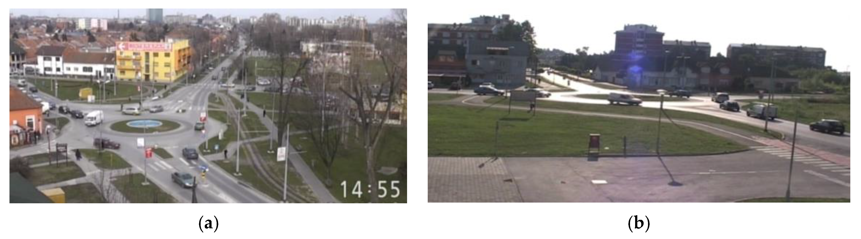
Two roundabouts enabled a comparison of field measurements and modelling results obtained with different methods of calibration. The first roundabout was used for model calibration and validation methods with new sets of measured data (Figure 1a), while the second roundabout allowed for the final validation of the calibrated model (Figure 1b).

The first data collection (operational indicators, the number of vehicles and traffic distribution at the intersection) for the first observed roundabout was made in the peak hour of the working day (a Wednesday in March), in the period between 15:00 and 16:00 (the calibration set is shaded in the

Table 2. The measured values of the observed traffic indicators.

	First Roundabout			Second Roundabout
	3 March 15:00–16:00	3 March 16:00–17:00	14 July 14:00–15:00.	14 July 08:00–09:00
Mean value of traveling time (s)	21.8	19.9	18.1	13.3
Maximum queue (m)	26	21	15.5	23
Number of stops at the entrance	89	61	54	56

). Traffic data were collected by one-hour video camera recordings, and the mean values of the traffic indicators are shown in Table 2 (detailed in [19]). The shaded dataset measured in situ was used to calibrate the model. Model validation in the comparisons of the models was carried out with two new sets of measured data at the same location and with one set of measured data at another location, (i.e., the second observed roundabout).

3.2. Comparison of the Different Methods of Computer Program Calibration

The role of neural networks is to provide a predict-function of the VISSIM simulation output values. MATLAB code creates all possible sets of input parameters to be used by the predict-function. It is important to emphasize that the predict-function gives almost an instant result, while the direct application of the VISSIM in the analysis of all sets of input parameters would be extremely time consuming.

The model approximates the satisfactory real traffic conditions if the Equation (3) is fulfilled for one observed traffic indicator and Equation (4) for the three traffic indicators.

$$\left|\frac{T_{MOD}-T_{MEAS}}{T_{MEAS}}\right|\le 5\%$$

(3)

$$\left|\frac{T_{MOD}-T_{MEAS}}{T_{MEAS}}\right|\mathrm{AND}\left|\frac{Q{\max }_{MOD}-Qma{x}_{MEAS}}{Qma{x}_{MEAS}}\right|\mathrm{AND}\left|\frac{STO{P}_{MOD}-STO{P}_{MEAS}}{STO{P}_{MEAS}}\right|$$

(4)

where:

T_MOD is the mean value of the modelled traveling time between measurement points,

T_MEAS is the mean value of the measured traveling time between measurement points,

Qmax_MOD is the mean value of the modelled maximum queue at the entrance,

Qmax_MEAS is the mean value of the measured maximum queue at the entrance,

STOP_MOD is the mean value of the modelled number of stops at the entrance, and

STOP_MEAS is the mean value of the measured number of stops at the entrance.

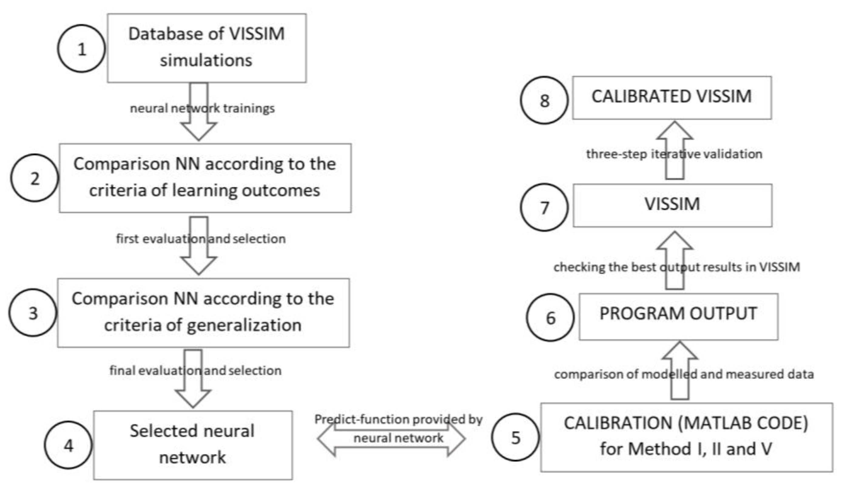
A scheme of a computer program for the calibration is shown in Figure 2. Databases of simulation results for observed traffic indicators were created in VISSIM, which was used for the training of the neural networks (step 1). Each of the four databases, on which the neural networks have been trained, consists of 1379 variations of model input parameter values.

All trained neural networks were compared according to the results achieved in the training and test database (step 2). In the process of validation, neural networks were examined according to the generalization capability of the new databases that were not used for the training of the neural networks (step 3). The predict-function of the neural networks that gave the most accurate prediction of the simulation results was used in a computer program of the microsimulation model calibration (steps 4 and 5 in Figure 2).

The comparison criterion of the modelled and measured values of traffic parameters created a set of potentially optimal combinations of the input parameter values in the calibration program output file (step 6). The final optimization of the input parameters from the set of potentially optimal solutions, generated by computer program, was performed on the basis of a comparison of the simulation results obtained by the original microsimulation traffic model (i.e., by VISSIM) and measuring the data in situ (steps 7 and 8 in Figure 2).

Different methods of computer program calibration were investigated and evaluated. The number of neural networks used for the prediction and the observed output parameter for each calibration method is shown in the

Table 3. Various applications of neural networks in the calibration.

Methods	Database of VISSIM Simulations	Input Parameters	Output Traffic Indicators	Neural Network	Response of Neural Network (Correlations) 1
Method I	Database I	8	1 (Travel time)	1	88%
Method II	Database II	8	3 (Travel time, max. queue, no. of stops)	1	83% 52% 45%
Method III	Database III	8	1 (Max. queue)	1	40%
Method IV	Database IV	8	1 (No. of stops)	1	52%
Method V	Database I, III and IV	8	3 (Travel time, max. queue, no. of stops)	3	88% 40% 52%

¹ Prediction of the neural network vs. VISSIM simulations on the trained database.

. Table 3 lists the correlations achieved by the neural network in relation to the target data, which are the results of the VISSIM simulation for the observed parameters.

Use of Neural Networks Prediction of the VISSIM Simulation

Within the present paper, four models were formed using neural networks, (Table 3). The last method of applying neural networks combines three previously created models in predicting traffic indicators.

The training of the neural networks and the analysis of the prediction results were made using the NeuroShell2 program. The following networks were tested: ward nets, standard nets, jump connection nets, Jordan–Elman nets and general regression net [20]. When creating a neural network learning database, the NeuroShell2 program can extract certain data percentages of the test dataset, which the network will not use for training but for the testing of the learning success on the training dataset (the remaining data of the database). In this analysis, 20% of the data obtained by random selection from the input database were used for the test dataset. For the back-propagation type of neural networks, the best prediction results were preserved for the test and training dataset. For the training dataset, the neural network gives predictions for the data about which it has learnt, whereas the test dataset is not available to the learning network and is used, therefore, for the evaluation of the network generalization ability. For regressive networks, the two network sub-types were analyzed: the adaptive and iterative network types.

The number of hidden layers and neurons in hidden layers varied due to the neural network reaction on the change of layers and number of neurons (better or worse prediction results). Altogether, 176 neural networks were analyzed during testing and evaluation of the optimal neural networks for prediction needs by all calibration methods. Neural networks (70) trained on Database I differed in architecture, the number of hidden layers, the number of neurons in hidden layers, and activation functions. Neural networks, 72 of them, were trained on Database II. Networks tested on Databases III (20) and IV (14) were selected on the basis of the results that they gave in Database II.

All trained neural networks were compared according to the results achieved on the training dataset (evaluation of the network trainings) by using the following criteria: correlation, mean absolute error, maximum absolute error and percentage of results with error smaller than 5%, detailed learning and generalization results of the trained neural networks shown in [20].

In the process of test validation (Figure 2), all networks were examined according to generalization capability (the ability to predict the unknown input data).

The final selection of the neural network, which gives the most accurate prediction of the simulation results for each database, was made on the basis of the validation results. The validation dataset consisted of 64 new combinations of input parameter values and output traffic parameters. Prediction error is calculated as the absolute difference value between prediction results obtained by the neural network and values obtained by the VISSIM simulation. The criterion for selection of a neural network to be used in the calibration procedure for each calibration method is a minimum mean absolute error on the validation dataset. The best results were achieved by the general regression neural network type for all databases on which the neural networks were trained.

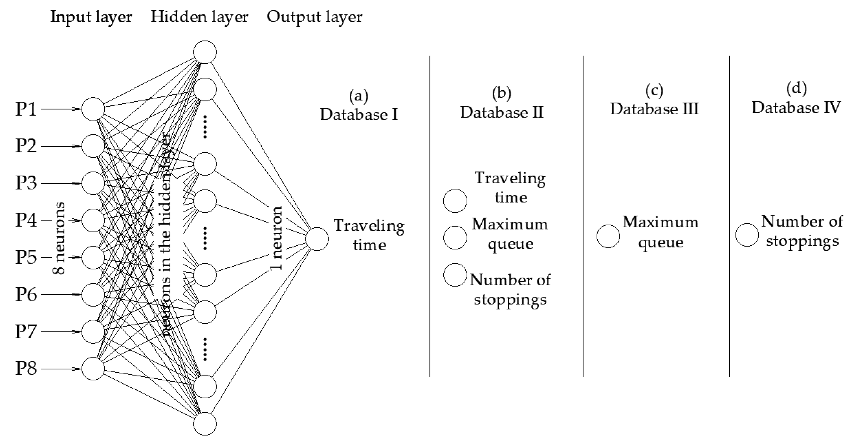
Networks that gave the best prediction results in relation to expected results (VISSIM simulation results) according to the criterion of the minimum mean absolute error were (Figure 3):

• Database I: General regression type networks, one hidden layer with 5500 neurons, modified activation function in the logistic function, an iterative type of network (GR5500-logist IT) (Figure 3a);
• Database II: General regression type networks, one hidden layer with 2500 neurons, modified activation function in logistic function, an iterative type of network (GR2500-logist IT) (Figure 3b);
• Database III: General regression type networks, one hidden layer with 2500 neurons, scale function-non, genetic, adaptive type of network, genetic breeding pool size 100 (GR2500-non AD100) (Figure 3c);
• Database IV: General regression type networks, one hidden layer with 2500 neurons, scale function-non, genetic, adaptive type of network, genetic breeding pool size 100 (GR2500-non AD100) (Figure 3d).

Method V using uses the predict-function of three neural networks of Databases I, III and IV.

Mathematical models (prediction-functions) generated by trained neural networks can be obtained in mathematical notation, but due to its length and complexity, it is not directly applicable in practice for calculating the prediction value (it is described in detail in [19]). In the calibration program, the predict-function was used as a subroutine in MATLAB, and it is possible to import the predict-function into Excel to check the prediction on an unknown dataset and evaluate the generalization of the model, which was carried out in the framework of this work on an independent database.

The calibration of the microsimulation model is a process aimed at fine-tuning the values of the input parameters that will give a minimum discrepancy between the simulated and measured traffic indicators.

In this study, the objective functions are formulated as mean absolute normalized error (MANE) [10] are provided by Equations (5)–(8).

$$\min MANE\left(T\right)=\frac{1}{N}{{\displaystyle \sum }}_{j=1}^N\left(\frac{\left|T_{mod}-T_{meas}\right|}{T_{meas}}\right)$$

(5)

$$\min MANE\left(Q_{max}\right)=\frac{1}{N}{{\displaystyle \sum }}_{j=1}^N\left(\frac{\left|Qma{x}_{mod}-Qma{x}_{meas}\right|}{Qma{x}_{meas}}\right)$$

(6)

$$\min MANE\left(STOP\right)=\frac{1}{N}{{\displaystyle \sum }}_{j=1}^N\left(\frac{\left|STO{P}_{mod}-STO{P}_{meas}\right|}{STO{P}_{meas}}\right)$$

(7)

$$\min MANE\left(T,Qmax,STOP\right)=\frac{1}{N}{{\displaystyle \sum }}_{j=1}^N\left(\frac{\left|T_{mod}-T_{meas}\right|}{T_{meas}}+\frac{\left|Qma{x}_{mod}-Qma{x}_{meas}\right|}{Qma{x}_{meas}}+\frac{\left|STO{P}_{mod}-STO{P}_{meas}\right|}{STO{P}_{meas}}\right)$$

(8)

The modeled and measured values of the observed traffic parameters were compared (explained in more detail in Section 3.2), and N is the number of observations. The objective Equations (5)–(7) were applied to Methods I, III and IV respectively, and the objective Equation (8) was applied to Methods II and V.

According to the correlations achieved by the neural network in relation to VISSIM (Table 3), Methods III and IV did not achieve satisfactory correlations, so they will not be further analyzed as potential calibration methods. The results obtained by Methods I, II and V are analyzed in detail below.

4. Results

4.1. Testing of the Output Program Results in VISSIM

The process of program calibration was achieved with MATLAB code, designed for the needs of each individually analyzed calibration method, discussed in more detail in [19]. The prediction-function obtained by training the neural network (NeuroShell2) was used as a sub-program in the calibration program. Output data files of each method were created for specified statistical criteria according to expression (3) for Method I and to expression (4) for Methods II and V. Correspondence evaluation (correspondence of datasets obtained by computer program calibration (output file) and the set of real VISSIM simulation values for the same values of input parameters) of each output dataset, which was based on actual VISSIM simulation results, was crucial for the assessment of the applicability of neural networks in the computer program calibration. Due to the size of the output dataset, the correspondence evaluation was made based on the dataset of 100 VISSIM simulations for each method, which can be considered only as a relative indicator intended for method comparison.

For Method I, which analyzed one traffic indicator—travel time, the results’ correspondence of the output dataset and actual VISSIM simulation values was 80%. If the set of potentially optimal combinations of input parameters with 80 combinations is analyzed in the context of calibration by queue parameters obtained by VISSIM simulations, it results in 13 combinations (

Table 4. Validation by the other traffic indicators (set I of the measured data)—Method I.

Combination of the Input Parameters								Neural Net. Prediction	VISSIM Result
P1	P2	P3	P4	P5	P6	P7	P8	T	T	Qmax	STOP
6	4	164	8	2.4	2	3.3	40	21.267	20.8	25	86
6	4	172	8	2.4	1.9	3.4	40	21.303	20.8	25	90
6	4	172	8	2.4	1.9	3.5	40	21.295	20.9	25	89
6	4	172	8	2.5	1.9	3.3	40	21.295	20.8	25	86
6	4	172	12	2.4	1.9	3.4	40	21.271	20.8	25	90
6	4	172	12	2.4	1.9	3.5	40	21.264	20.9	25	89
6	4	172	12	2.5	1.9	3.3	40	21.283	20.8	25	86
6	4	173	8	2.4	1.9	3.4	40	21.298	21.1	25	85
6	4	173	12	2.4	1.9	3.4	40	21.298	21.1	25	85
6	4	175	8	2.5	1.9	3.5	40	21.262	21.0	25	85
6	4	176	8	2.4	1.8	3.5	40	21.275	21.4	27	88
6	4	176	8	2.5	1.8	3.4	40	21.273	20.9	27	90
6	4	176	12	2.5	1.8	3.4	40	21.273	20.9	27	90

) of input parameters that satisfy all three indicators according to expression (4). In the field, measured maximum queue for the calibration dataset was 26 m and number of stoppings at the entrance was 89 (Table 2).

Combinations of the input parameters that were the closest to the measured values in situ (21.8 s) are shaded in Table 3. Two bolded combinations of input parameters, which present the best result, entered the second step of the evaluation procedure. The value of the simulated time of 21.4 s was the best result and, for the second combination, one of two practically identical combinations was selected. VISSIM, unlike neural networks, gave the same values of traffic indicators (P4 = 8 and P4 = 12), such that one of two combinations, which differs only by the fourth input parameter P4, was selected.

For Method II, the correspondence of all three parameters was 2% for the output data file of Method II (

Table 5. The best combinations of input parameters of Method II.

Combination of the Input Parameters								Neural Network Prediction			VISSIM Result
P1	P2	P3	P4	P5	P6	P7	P8	T	Qmax	STOP	T	Qmax	STOP
9	4	250	0	2.1	3.1	3.8	40	20.18	24.72	80.13	20.9	25	87
9	4	250	0	2.1	3.1	4.0	40	20.20	24.72	80.16	20.8	25	87

), and for the output files of Method V, was 7% (

Table 6. The best combinations of input parameters of Method V.

Combination of the Input Parameters								Neural Network Prediction			VISSIM Result
P1	P2	P3	P4	P5	P6	P7	P8	T	Qmax	STOP	T	Qmax	STOP
9	2	247	8	2.1	2.7	4.3	40	20.94	24.71	85.31	20.8	27	88
9	2	266	8	2.1	2.8	4.3	40	20.94	24.71	85.31	21.0	25	86
9	2	272	8	2.1	2.9	4.2	40	20.93	24.71	85.96	21.3	25	87
9	2	264	8	2.1	2.8	4.2	40	20.93	24.71	85.96	20.9	25	85
9	2	254	8	2.1	2.8	4.3	40	20.92	24.751	85.31	20.8	25	87
9	2	264	8	2.1	3.1	4.3	40	20.92	24.71	85.31	21.3	25	91
9	2	255	8	2.1	2.7	4.2	40	20.92	24.71	85.96	21.3	25	86

).

An interesting insight can be obtained by analyzing the number of vehicles that the model could not generate in the designated simulation time (one hour). Having in mind that the recorded number of vehicles de facto went through the roundabout in real field conditions in the examined time interval, it can be concluded that some combinations of input parameter values significantly reduce the modelled capacity of the intersection.

The final selection criterion for the two combinations by Method V was the magnitude of simulation error, which VISSIM registered after a one-hour simulation. The microsimulation tool reported an error for all three combinations, failing to generate any of the vehicles during the simulation process. For a small number of vehicles, it is generally not a problem because VISSIM does not simulate the exact number of vehicles, only the traffic distribution of the vehicles. For the first combination of input parameters, the model did not generate eight vehicles and, for the third, 10. Yet, this did not significantly change the final traffic image. For the second parameter combination, however, the model did not generate 35 vehicles, which means that the combination of input parameters reduces the capacity of the roundabout and, after all, might have affected simulated traffic indicators. Therefore, the first and third shaded combinations of input parameters were selected for the validation procedure.

4.2. Methods Validation by Comparison of VISSIM Simulation Results and Measured Indicators

The first validation was performed at the same roundabout at which the calibration procedure was carried out. The first dataset of traffic parameters for the validation was measured on a Wednesday in March, between 16:00 and 17:00. Measured values of traffic parameters and values obtained by VISSIM simulation for default values of input parameters, as well as the two best parameter combinations obtained by each calibration method, are shown and compared in

Table 7. Comparison of the traffic indicators—first validation.

Input Parameters of the VISSIM Model								Traffic Indicators
P1	P2	P3	P4	P5	P6	P7	P8	T	Qmax	STOP
Measured Values
								19.9	21	61
Values Obtained by the VISSIM Model Simulations
Default Values of the Input Parameters
5	2	250	0	2	2	3	40	20.3	15	60
Method I
6	4	176	8	2.4	1.8	3.5	40	19.8	22	58
6	4	173	8	2.4	1.9	3.4	40	20.2	15	63
Method II
9	4	250	0	2.1	3.1	3.8	40	19.9	19	63
9	4	250	0	2.1	3.1	4.0	40	20.0	15	55
Method V
9	2	272	8	2.1	2.9	4.2	40	20.2	15	57
9	2	255	8	2.1	2.7	4.2	40	19.6	15	52

.

For the first validation procedure, simulation results closest to the measured values were provided by the combination of input parameters obtained by calibration, according to Method I (shaded in Table 7).

The second validation model (the comparison of the measured and simulated values) was based on the data measured on a Wednesday in July, between 14:00 and 15:00, at the same location at which the calibration was performed (

Table 8. Comparison of the traffic indicators—second validation.

Input Parameters of the VISSIM Model								Traffic Indicators
P1	P2	P3	P4	P5	P6	P7	P8	T	Qmax	STOP
Measured Values
								18.1	15.5	54
Values Obtained by the VISSIM Model Simulations
Default Values of the Input Parameters
5	2	250	0	2	2	3	40	17.6	23	50
Method I
6	4	176	8	2.4	1.8	3.5	40	17.6	15	52
6	4	173	8	2.4	1.9	3.4	40	17.8	15	53
Method II
9	4	250	0	2.1	3.1	3.8	40	17.6	24	46
9	4	250	0	2.1	3.1	4.0	40	17.5	24	44
Method V
9	2	272	8	2.1	2.9	4.2	40	18.0	24	50
9	2	255	8	2.1	2.7	4.2	40	18.3	24	52

). Table 8 shows that default values of the input parameters resulted in correct simulation results for traveling time; this was not the case with the queue parameters, which did not enter specified statistical limits. Both parameter combinations obtained by calibration procedures of Method I (shaded) satisfied the limit set by expression (4) when approaching the values measured in the field.

The third validation was made at the new location, the second observed roundabout (Figure 1b). The second observed intersection is an urban one-lane roundabout, with similar geometric characteristics and the same functional level as the first roundabout. Both roundabouts introduce traffic from the express city road into the city network. The measured traffic indicators for the second intersection are presented in Table 2. Data were collected and traffic parameters measured on a Wednesday morning in July, between 08:00 and 09:00. Traffic volume, distribution and traffic structure for both roundabouts are presented in more detail in [19]. VISSIM simulation values for the default values of the input parameters and the two best parameter combinations, which were obtained by each calibration method, were compared with measured values of traffic parameters and are presented in

Table 9. Comparison of the traffic indicators—third validation.

Input Parameters of the VISSIM Model								Traffic Indicators
P1	P2	P3	P4	P5	P6	P7	P8	T	Qmax	STOP
Measured Values
								13.3	23	56
Values Obtained by the VISSIM Model Simulations
Default Values of the Input Parameters
5	2	250	0	2	2	3	40	13.1	27	50
Method I
6	4	176	8	2.4	1.8	3.5	40	13.1	22	58
6	4	173	8	2.4	1.9	3.4	40	13.1	22	54
Method II
9	4	250	0	2.1	3.1	3.8	40	13.6	21	62
9	4	250	0	2.1	3.1	4.0	40	13.7	21	64
Method V
9	2	272	8	2.1	2.9	4.2	40	13.6	20	63
9	2	255	8	2.1	2.7	4.2	40	13.6	22	65

.

Default values of the input parameters gave simulation values of traveling time within specified limits, but the queue parameter results were not within the expected range. Both parameter combinations obtained by calibration procedures of Method I (shaded) satisfied the limit set by expression (4) for the second roundabout.

The iterative evaluation process of the calibration results is presented in Table 7, Table 8 and Table 9. The overview of the obtained simulation results with default input parameters, as well as two selected combinations of input parameters of each calibration method, gave the summary presented in

Table 10. Summary evaluation of the simulated traffic parameters in relation to the measured ones.

	Default			Method I						Mathod II						Method V
	Time	Queue		Time		Queue				Time		Queue				Time		Queue
	T	Qmax	STOP	T		Qmax		STOP		T		Qmax		STOP		T		Qmax		STOP
				1 1	2 2	1	2	1	2	1	2	1	2	1	2	1	2	1	2	1	2
Calibration	✕	✕	✕	✓	✓	✓	✓	✓	✓	✓	✓	✓	✓	✓	✓	✓	✓	✓	✓	✓	✓
Validation I	✓	✕	✓	✓	✓	✓	✕	✓	✓	✓	✓	✕	✕	✓	✕	✓	✓	✕	✕	✕	✕
Validation II	✓	✕	✕	✓	✓	✓	✓	✓	✓	✓	✓	✕	✕	✕	✕	✓	✓	✕	✕	✕	✓
Validation III	✓	✕	✕	✓	✓	✓	✓	✓	✓	✓	✓	✕	✕	✕	✕	✓	✓	✕	✓	✕	✕

¹ first selected combination of input parameters; ² second selected combination of input parameters.

. Traffic parameter values, which met the statistical criteria set by mathematical expression (4) are indicated by a tick (✓), while those that did not are indicated by a cross mark (✕).

Table 10. shows that the combination of input parameters with default values that give the biggest differences between the simulation values in relation to the measured ones.

It is evident from Table 10 that both combinations of input parameters obtained by all calibration methods for the output indicator of the traveling time gave simulation values within the pre-set statistical criterion (3).

By analyzing and comparing the results of the traffic parameter values shown in Table 7, Table 8 and Table 9, and particularly by analyzing summary Table 10, one can notice the combination of input parameters that satisfied all of the observed indicators within the pre-set limits, which is the first combination of input parameters obtained by the calibration procedure in Method I (Table 10, shaded), according to expression (4).

The optimal parameter values of the VISSIM simulation model obtained by the calibration and the iterative validation procedure for single-lane roundabouts in Osijek are shown in

Table 11. Optimal values of the VISSIM input parameters for single-lane roundabouts.

Optimal Values of the VISSIM Model Input Parameters
P1 Simulation resolution	6
P2 Number of observed proceeding vehicles	4
P3 Maximum looking ahead distance (m)	176
P4 Minimum looking ahead distance (m)	8
P5 Average standstill distance (m)	2.4
P6 Additive part of the desired safety distance (m)	1.8
P7 Multiplicative part of the desired safety distance (m)	3.5
P8 Desired speed	40

.

The analysis of the influence of each individual input parameter on the prediction result given by the neural network, which is presented in more detail in [19], did not eliminate parameter 2, but its influence in the application of the microsimulation model was not significant.

According to the obtained results at the new location, the second observed roundabout (Table 8), the optimal combination of parameters is applicable to the reference problem (single-lane roundabout) in the local condition, and is not only applicable on the roundabout that was used for model calibration.

4.3. Statistical Comparison of the Raw Datasets of the Simulated and Measured Data

The dataset of measured travel times between the selected measuring points was formed in a one-hour recording of the roundabout. The left turn traffic flow was chosen, because it takes the longest time in the roundabout, has the lowest speed, and shows the greatest sensitivity to the design elements of the intersection.

Bearing in mind the stochastic nature of the traffic flow, various scenarios of vehicle arrivals in the observed time of one hour were analyzed using a calibrated model. The travel time dataset obtained by simulation was formed as the mean value of ten different vehicle arrival scenarios, the initial value of the random number generator (random seed) was 42, and the increment was 10.

In all observed scenarios, the same measurable elements of traffic regulation were used, which have a significant impact on traffic conditions, such as the actual timetable of trams and buses for public transport. The tram line passes over the observed incoming traffic lane into the roundabout (Figure 1a), which significantly affects the dynamic characteristics of the incoming flows of the observed traffic flow of vehicles.

Near the observed roundabout there is an intersection with traffic lights, which, due to its location has a significant influence on the traffic flows of the observed roundabout, so the traffic lighted intersection is included in the model of the observed roundabout. In the simulations, a real signal program of the traffic light regulation was used, which regulates the traffic at the intersection near the observed roundabout and has an impact on the incoming and outgoing flows of vehicles.

Table 12. Basic statistical indicators for the measured and simulated travel times.

	N	Mean	StDev	Median	Min	Max	A–D Test	p-Value
Measured	135	21.8	6.046	21.00	12.00	43.00	2.952	<0.005
Simulated	135	21.4	5.875	20.00	12.00	40.00	4.306	<0.005

shows the basic statistical indicators for the measured and simulated travel times simulated with the calibrated VISSIM, for all vehicles of the observed traffic flow in the roundabout.

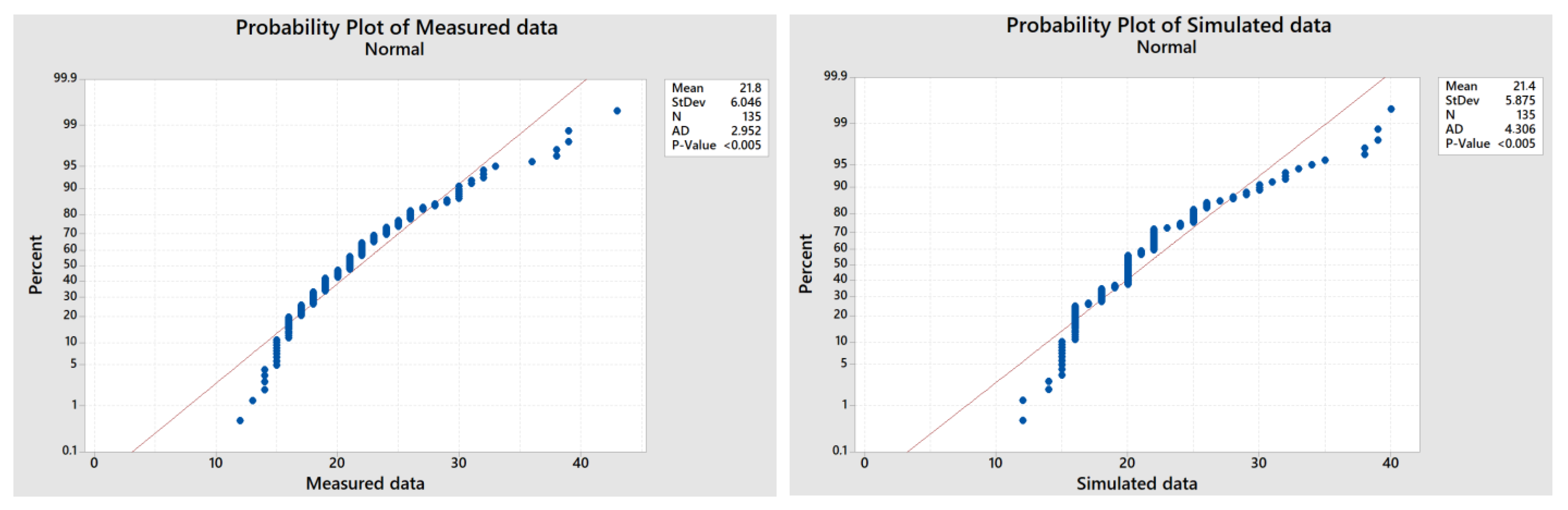
The normality of the data distribution test for the two observed datasets serves as an initial test for choosing a statistical test for comparing two observed datasets.

The normality of the data distribution for the two observed datasets was tested by performing the Anderson–Darling test. The null hypothesis of the test is that data follow a normal distribution and a significance level of 0.05 was set. The probability plot for each dataset is shown in Figure 4. According to the results of the Anderson–Darling test (Table 12, Figure 4), the p-value is less than the set threshold and the null hypothesis is rejected, which means none of the groups of observed data follow a normal distribution.

A parametric test (ANOVA) is applied to the normally distributed data, but according to the results, it is necessary to apply non-parametric tests, such as Bonett and Levene, for comparison. Datasets of measured and simulated travel times were compared with the aim of determining whether they are statistically significantly different or not. The null hypothesis was set that the relationship between the standard deviations and the variance of the two observed datasets is equal to 1, and a significance level of 0.05 was set. The results are presented in

Table 13. Standard deviations and variances.

	StDev	Ratio	Variance	Ratio
Measured	6.046	1.029	36.549	1.059
Simulated	5.875		34.510

and

Table 14. Statistical test results.

Method	Statistic Test	p-Value	CI for StDev Ratio	CI for the Variance Ratio
Bonett	0.06	0.806	0.816; 1.302	0.666; 1.695
Levene	0.43	0.514	0.857; 1.369	0.735; 1.874

CI—95% Confidence Intervals.

.

According to the results shown in Table 14, the null hypothesis cannot be rejected, which means that the difference between the two observed datasets is not statistically significant.

5. Discussion

By reviewing the literature (Section 2), it is possible to see a significant diversity in the approach to the calibration of microsimulation traffic models. Of the applied calibration algorithms, the genetic algorithm prevails. The methodological approach of applying neural networks has proven to be effective [15] and within the framework of this paper, different methods of applying neural networks in the process of calibrating a microsimulation traffic model were analyzed.

From the initial five, three methods of application of neural networks in the calibration were analyzed in detail. Calibration methods varied in the number of output traffic indicators predictable by a neural network and number of neural networks used in the program calibration procedure. Altogether, 176 predictive neural networks were trained and analyzed within the NeuroShell2 program. Each database for neural networks training has 1379 combinations of input parameters and output operational indicators of VISSIM simulations. The paper [20] presents the results of the comparison of learning results on the training dataset of all trained networks according to selected criteria. The neural network for each calibration method was chosen by the two-step evaluations (results of learning and generalization) of neural networks.

The process of program calibration was realized in the MATLAB program designed for the needs of each individually analyzed calibration method [19]. The exported prediction-function obtained by training the neural network (NeuroShell2) was used as a subroutine in the calibration program.

Model validation is the evaluation of calibration model efficiency by comparison of modelled and measured traffic parameters. The basic requirement, that every calibrated traffic microsimulation model must meet, is that it can be successfully validated with a new set of data of the same type, in this case traveling time between the measurement points. A higher standard of validation is reached if the model calibrated for traveling times data also gives good estimates of other parameters, such as queue parameters [21].

The validation activity in this research was performed iteratively, in three steps. For all three methods, there were three validations based on the comparison of correspondence aggregate data of the simulation results obtained by the calibrated VISSIM and new sets of measured data. Two validations were conducted at the same location at which the calibration was carried out. The third validation was performed at the new location in order to verify the applicability of selected parameters on the type of considered intersection, rather than only at the location where the calibration was carried out.

Validation of the computer program calibration method led to the selection of the optimal combination of input parameter values of the VISSIM model.

The comparison and evaluation of mean values of the simulation parameter in relation to those measured in the field for all field datasets is shown in Table 10. The method that gave the optimal combination of input parameters was the neural network-based method, which provided the prediction for the traveling time between the selected measurement points.

According to the results in Table 7, Table 8, Table 9 and Table 10, it was shown that the calibration method that uses travel time as a traffic indicator gives good results for the queue parameters, which were not used in the calibration procedure. This is a somewhat unexpected result, because the other two methods use neural network predictions for travel time and queue parameters in the calibration process. The result is nevertheless logical, when taking into account the results in Table 3, which show that the neural network does not give a good prediction for the queue parameters, while for the prediction of the travel time it gives a good correlation with the VISSIM data. The neural network that served as a prediction tool for the mentioned calibration method achieved the best correlation on the training dataset (88.3%) and generalization, i.e., the best prediction of traffic indicators on unknown data (it had the lowest mean absolute error).

The last step of the model validation made in this research is the analysis of disaggregated data for measured and simulated travel times of observed vehicle traffic flow, using statistical tools. The set of data obtained by simulation with a calibrated model is the mean value of ten different traffic scenarios of vehicle arrivals, in accordance with the stochastic nature of the traffic flow. Bearing in mind that the observed datasets do not follow a normal distribution, the Bonett and Levene tests for two variances and standard deviations were applied. According to the results of the conducted statistical tests, the difference between the two observed datasets is not statistically significant. This result is the expected confirmation of earlier results of the validation of the calibration method.

In the continuation of the research, the calibration methodology using neural networks was applied to another type of intersection in another city with significantly different local conditions and the results proved to be equally good in calibrating the microsimulation model.

6. Conclusions

The best insight into the success of the calibration of the model provides a comparison of the simulated and measured traffic indicators. For this study, we created four sets of measured data in two single-lane roundabouts. Measurement of traffic data in situ was made in real-life traffic conditions, measuring and recording traffic with a video camera for a period of one hour. Comparison of the measured data and those obtained by simulation with a calibrated and uncalibrated microsimulation model was also conducted. This paper presents the results of the comparison of different methods of neural network approaches for the calibration of microsimulation traffic models. From the initial five methods of applying neural networks in the calibration process, three methods were selected for detailed analysis according to the criterion of good correlation for at least one traffic indicator. The research results show that neural networks are applicable in the calibration of microsimulation traffic models.

The results lead to the following conclusions:

• The first combination of input parameters values of Method I satisfied the statistical criteria set by expression (4) for all validation procedures;
• Results of the simulated values of the output indicator, travel time, satisfied the statistical criteria by expression (3) according to all methods; and
• Simulation results with default values of input parameters least corresponded with the measured values.

The combination of input parameters (Table 11) that satisfied the statistical criteria set by expression (4) in each validation procedure with aggregate data, was the first combination of parameters obtained by a calibration method that uses neural network prediction for travel time. This method was based on the neural network that achieved the best correlation with the VISSIM simulations on the training dataset (88.3%) and which gave the smallest mean absolute error in the generalization procedure. This method, based on the VISSIM example, is generally recommended for use in the process of program calibration of traffic microsimulation models.

According to the obtained results, the optimal combination of parameters is applicable to the reference problem (single-lane roundabout) and is not locally conditioned (only on the observed roundabout). Such a conclusion should be taken with caution, considering the fact that this research was based only on two single-lane roundabouts. In that sense, the possibility of generalization of the obtained values of input parameters on other types of roundabouts, or intersections in local conditions in general, should be further researched. The most calibrated input parameters are related to drivers’ behavior (psychology), which is always territorially and culturally conditioned.

The other two researched methods of computer program calibration which are based on the simultaneous calibration of several traffic indicators, open the door to further research into appropriate configurations of neural networks that can provide a better correlation for queue parameters.

Table 6, Table 7, Table 8 and Table 9 show that the model calibrated with a recommended method of calibration gave simulation results that differ from the measured data for less than 5%, for all sets of measured data and for all observed traffic indicators.

To evaluate the difference between the two sets of disaggregated data for the measured and simulated travel times with the calibrated model, statistical tests were used and the results showed that there is no statistically significant difference between the two sets of data.

The scientific contribution of this article is that it analyzes in detail different methods of applying neural networks in the process of calibrating a traffic microsimulation model. The use of neural networks in the calibration process is an innovative methodological approach (Table 1) which, according to the obtained results, has potential.

The weaknesses of this research are that only two roundabouts were analyzed, which does not provide enough breadth for generalizing the conclusions. The neural networks used in this research are those available in NeuroShell2 expert software. It should certainly be taken into account that some other tools are available in the research of the optimal type and configuration of neural networks, which should be further investigated.

Comparison results of the modelled and measured data show that the calibrated VISSIM microsimulation model, by using a neural network, was able to provide modelling results that reflected real traffic characteristics at observed roundabouts in local conditions.

References

- Flötteröd, G.; Bierlaire, M.; Nagel, K. Bayesian demand calibration for dynamic traffic simulations. Transp. Sci. 2012, 45, 541–561. [Google Scholar] [CrossRef]
- Shahdah, U.; Saccomanno, F.; Persaud, B. Application of traffic microsimulation for evaluating safety performance of urban signalized intersections. Transp. Res. Part C Emerg. Technol. 2015, 60, 96–104. [Google Scholar] [CrossRef]
- Llorca, C.; Moreno, A.T.; Lenorzer, A.J. Casas and A. Garcia. Development of a new microscopic passing manoeuvre model for two-lane rural roads. Transp. Res. Part C Emerg. Technol. 2015, 52, 157–172. [Google Scholar] [CrossRef]
- Chen, C.; Zhao, X.; Liu, H.; Ren, G.; Zhang, Y.; Liu, X. Assessing the Influence of Adverse Weather on Traffic Flow Characteristics Using a Driving Simulator and VISSIM. Sustainability 2019, 11, 830. [Google Scholar] [CrossRef]
- Fang, X.; Li, H.; Tettamanti, T.; Eichberger, A.; Fellendorf, M. Effects of Automated Vehicle Models at the Mixed Traffic Situation on a Motorway Scenario. Energies 2022, 15, 2008. [Google Scholar] [CrossRef]
- Park, B.; Qi, H. Development and Evaluation of Simulation Model Calibration Procedure. Transp. Res Rec. 2005, 1934, 208–217. [Google Scholar] [CrossRef]
- Kim, S.J. Simultaneous Calibration of a Microscopic Traffic Simulation Model and OD Matrix. Ph.D. Thesis, Texas A&M University, College Station, TX, USA, 2006. [Google Scholar]
- Paz, A.; Molano, V.; Martinez, E.; Gaviria, C.; Arteaga, C. Calibration of traffic flow models using a memetic algorithm. Transp. Res. Part C Emerg. Technol. 2015, 55, 432–443. [Google Scholar] [CrossRef]
- Chiappone, S.; Giuffrè, O.; Granà, A.; Mauro, R.; Sferlazza, A. Traffic simulation models calibration using speed–density relationship: An automated procedure based on genetic algorithm. Expert Syst. Appl. 2016, 44, 147–155. [Google Scholar] [CrossRef]
- Yu, M.; Wei, D.F. Calibration of microscopic traffic simulation models using metaheuristic algorithms. Int. J. Transp. Sci. Technol. 2017, 6, 63–77. [Google Scholar] [CrossRef]
- Sacks, J.; Rouphail, N.; Park, B.; Thakuriah, P. Statistically Based Validation of Computer Simulation Models in Traffic Operations and Management. J. Transp. Stat. 2002, 5, 1–24. [Google Scholar]
- Toledo, T.; Ben-Akiva, M.E.; Darda, D.; Jha, M.N.; Koutsopoulos, H.N. Calibration of microscopic traffic simulation models with aggregate data. Transp. Res. Rec. 2004, 1876, 10–19. [Google Scholar] [CrossRef] [Green Version]
- Cunto, F.; Saccomanno, F.F. Calibration and validation of simulated vehicle safety performance at signalized intersections. Accid. Anal. Prev. 2008, 40, 1171–1179. [Google Scholar] [CrossRef] [PubMed]
- Flötteröd, G.; Chen, Y.; Nagel, K. Behavioral calibration and analysis of a large-scale travel microsimulation. Netw. Spat. Econ. 2011, 12, 481–502. [Google Scholar] [CrossRef]
- Ištoka Otković, I.; Tollazzi, T.; Šraml., M. Calibration of microsimulation traffic model using neural network approach. Expert Syst. Appl. 2013, 40, 5965–5974. [Google Scholar] [CrossRef]
- Severino, A.; Pappalardo, G.; Curto, S.; Trubia, S.; Olayode, I.O. Safety Evaluation of Flower Roundabout Considering Autonomous Vehicles Operation. Sustainability 2021, 13, 10120. [Google Scholar] [CrossRef]
- Tollazzi, T.; Renčelj, M.; Turnšek, S. New type of roundabout: Roundabout with “depressed” lanes for right turning-“Flower roundabout”. Promet-Traffic Transp. 2011, 23, 353–358. [Google Scholar] [CrossRef]
- Pan, B.; Luo, S.; Ying, J.; Shao, Y.; Liu, S.; Li, X.; Lei, J. Evaluation and Analysis of CFI Schemes with Different Length of Displaced Left-Turn Lanes with Entropy Method. Sustainability 2021, 13, 6917. [Google Scholar] [CrossRef]
- Ištoka Otković, I. Using Neural Networks in the Process of Calibrating the Microsimulation Models in the Analysis and Design of Roundabouts in Urban Areas. Ph.D. Thesis, University of Maribor, Faculty of Civil Engineering, Maribor, Slovenia, 2011. [Google Scholar]
- Ištoka Otković, I.; Varevac, D.; Šraml., M. Analysis of neural network responses in calibration of microsimulation traffic model. Adv. Civ. Eng. 2015, 6, 67–76. [Google Scholar] [CrossRef]
- Hollander, Y.; Liu, R. The principles of calibrating traffic microsimulation models. TRANS 2008, 35, 347–362. [Google Scholar] [CrossRef]
Figure 1.
Observed roundabouts. (a) First roundabout; (b) second roundabout.
Figure 2.
Scheme of the computer program calibration.
Figure 3.
Neural network architecture used for the databases: (a) Database I; (b) Database II; (c) Database III; (d) Database IV.
Figure 4.
The probability plot for the measured and simulated data.