
Driving Behaviour and Usability: Should In-Vehicle Speed Limit Warnings Be Paired with Overhead Gantry?


Abstract
:1. Introduction
2. Method
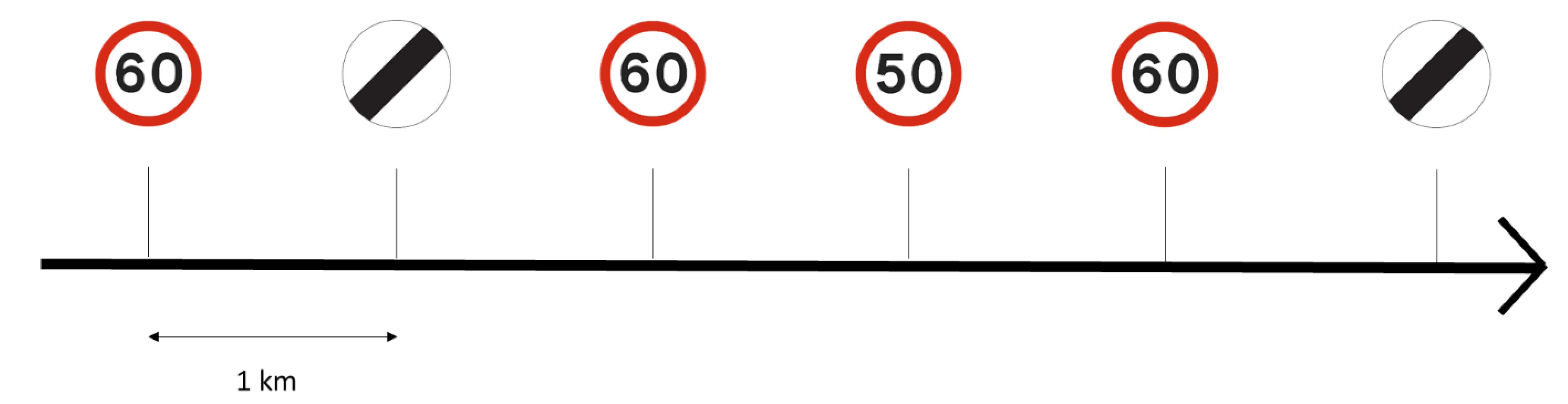
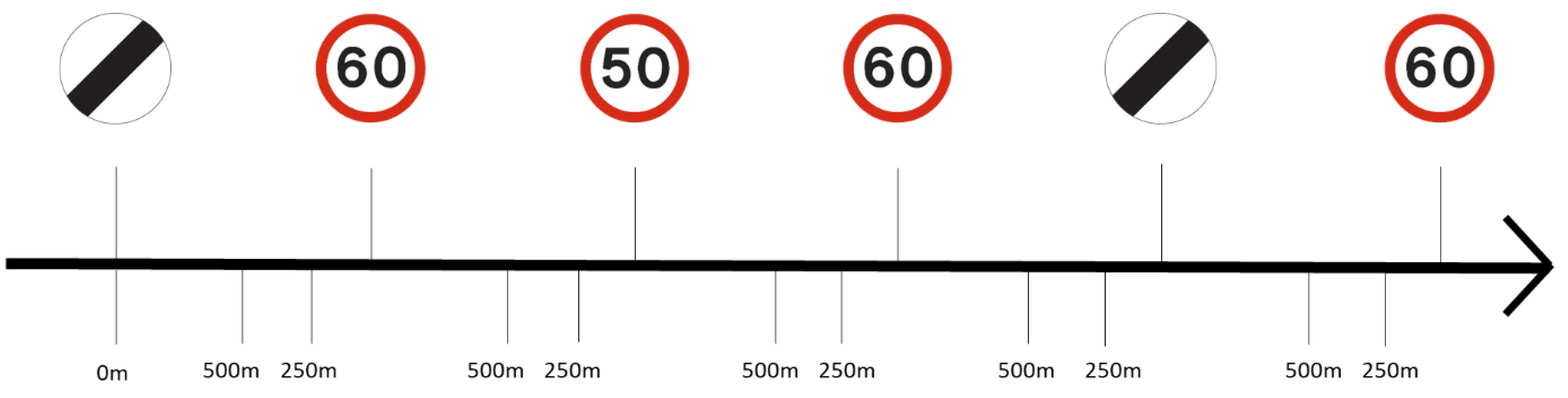
2.1. Experimental Design
2.2. Procedure
2.3. Participants
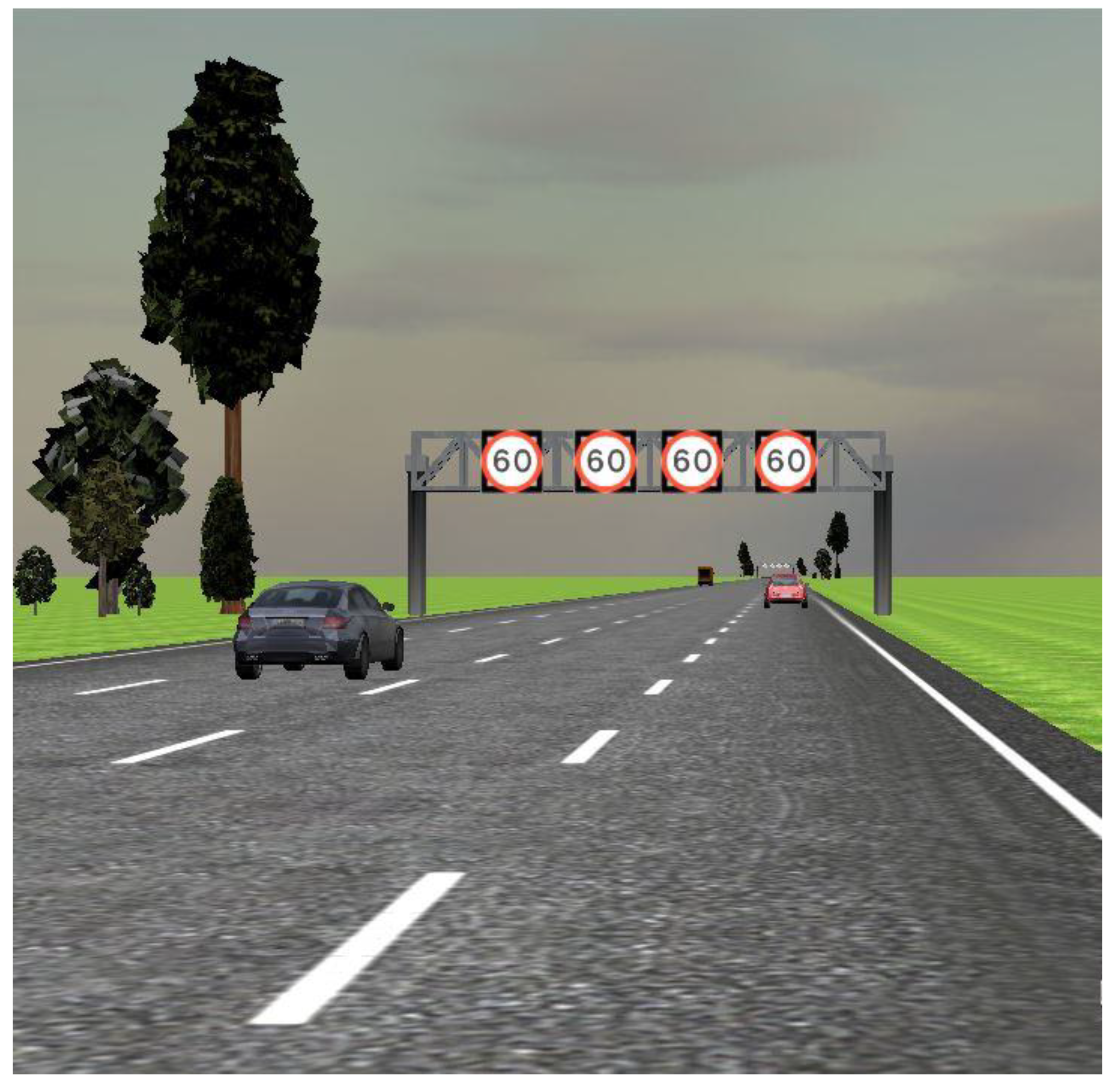
2.4. Simulator Equipment
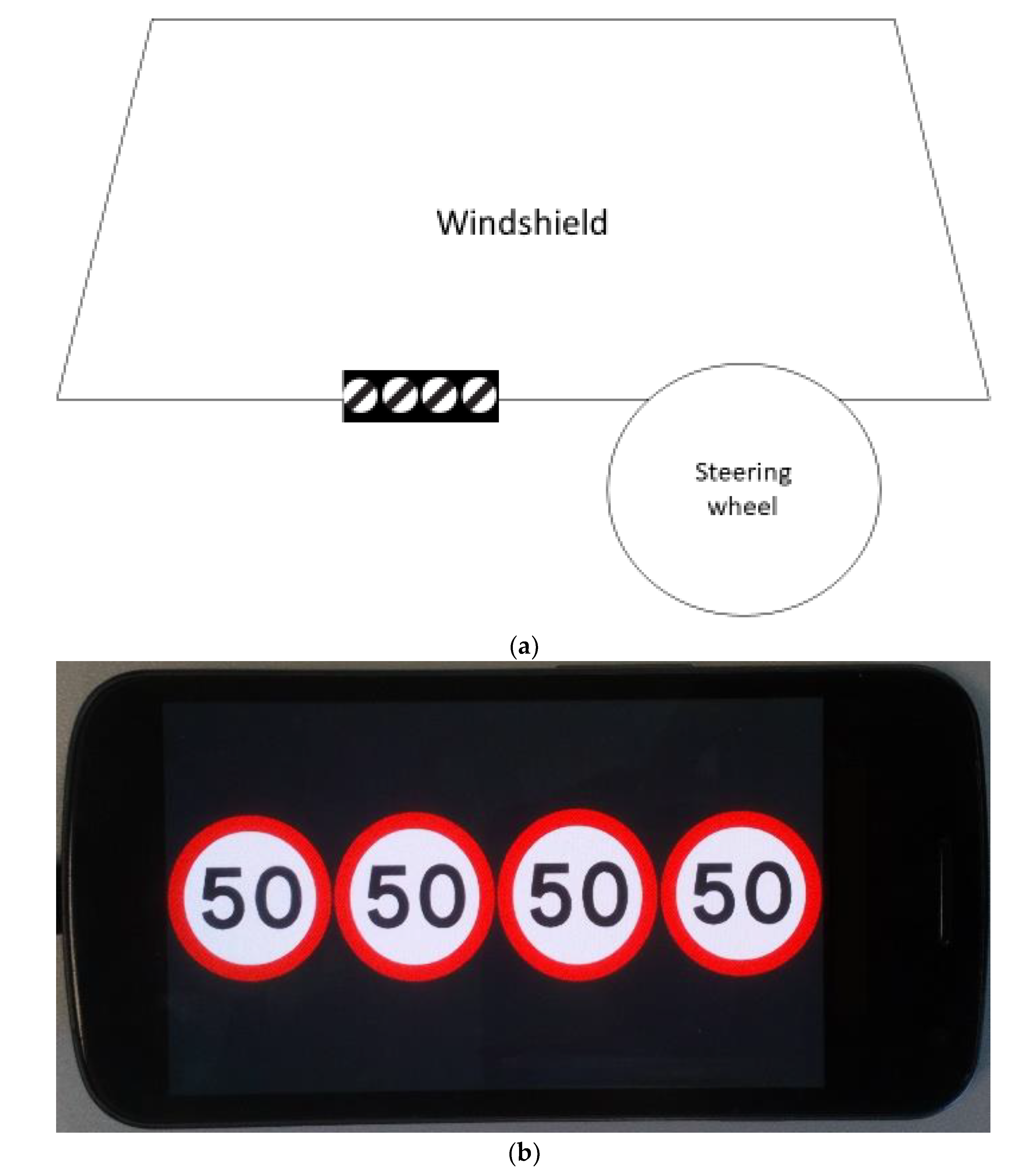
2.5. Human–Machine Interface
3. Measures
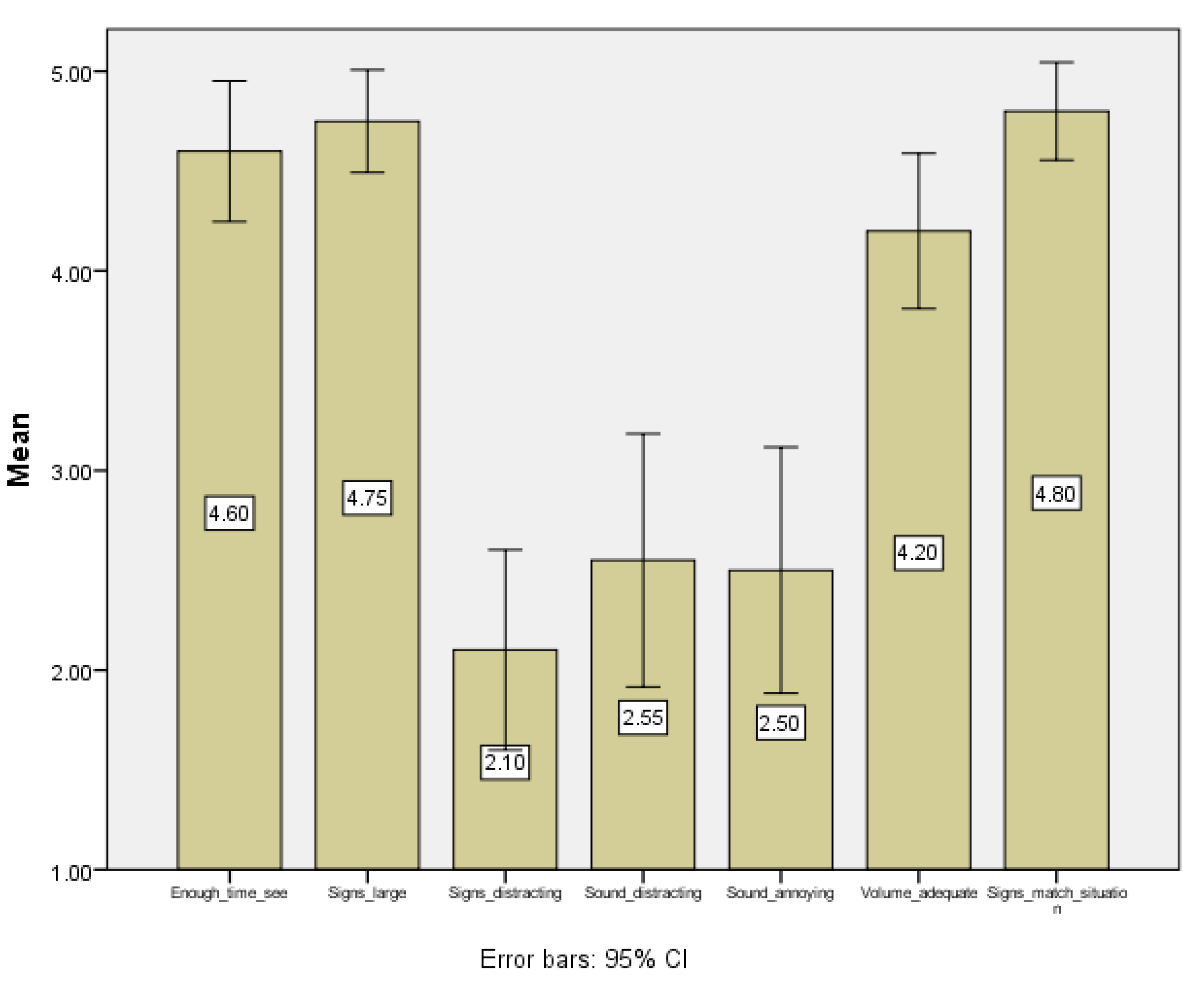
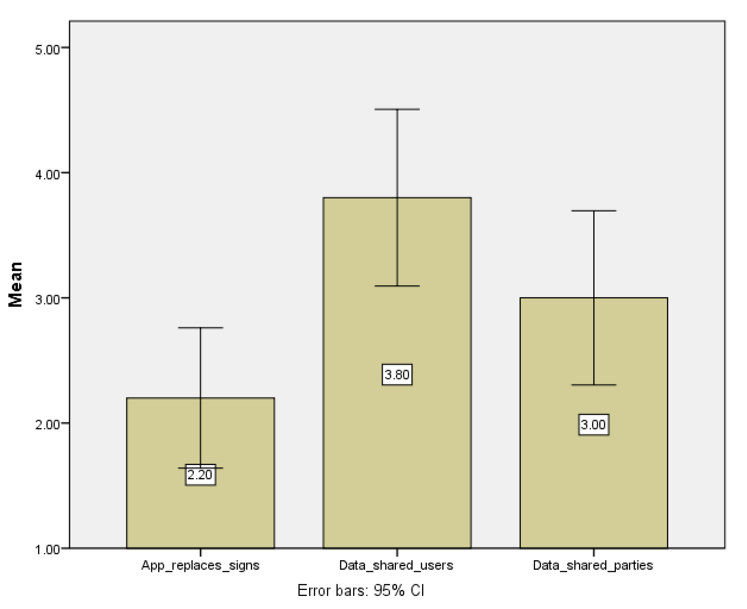
3.1. Questionnaire
- -
- I would mind if using an app that replaces the gantry and road signs every time I drive was mandatory,
- -
- I would be happy if an app replaces the gantry and road signs,
- -
- I would be happy if the driving-related data collected by my car was shared with other road users,
- -
- I would be happy if the driving-related data collected by my car was shared with other parties (app and vehicle manufacturers, local transport authorities, traffic management).
- -
- The warnings’ location in the vehicle was appropriate;
- -
- I would like to be told what the warnings mean before seeing them while driving;
- -
- I had enough time to see the warnings on the mobile phone;
- -
- I had been distracted by these warnings;
- -
- I found the signs were congruent with what happened on the road.
3.2. Driving Behaviour
4. Results
4.1. Usability and Data-Sharing
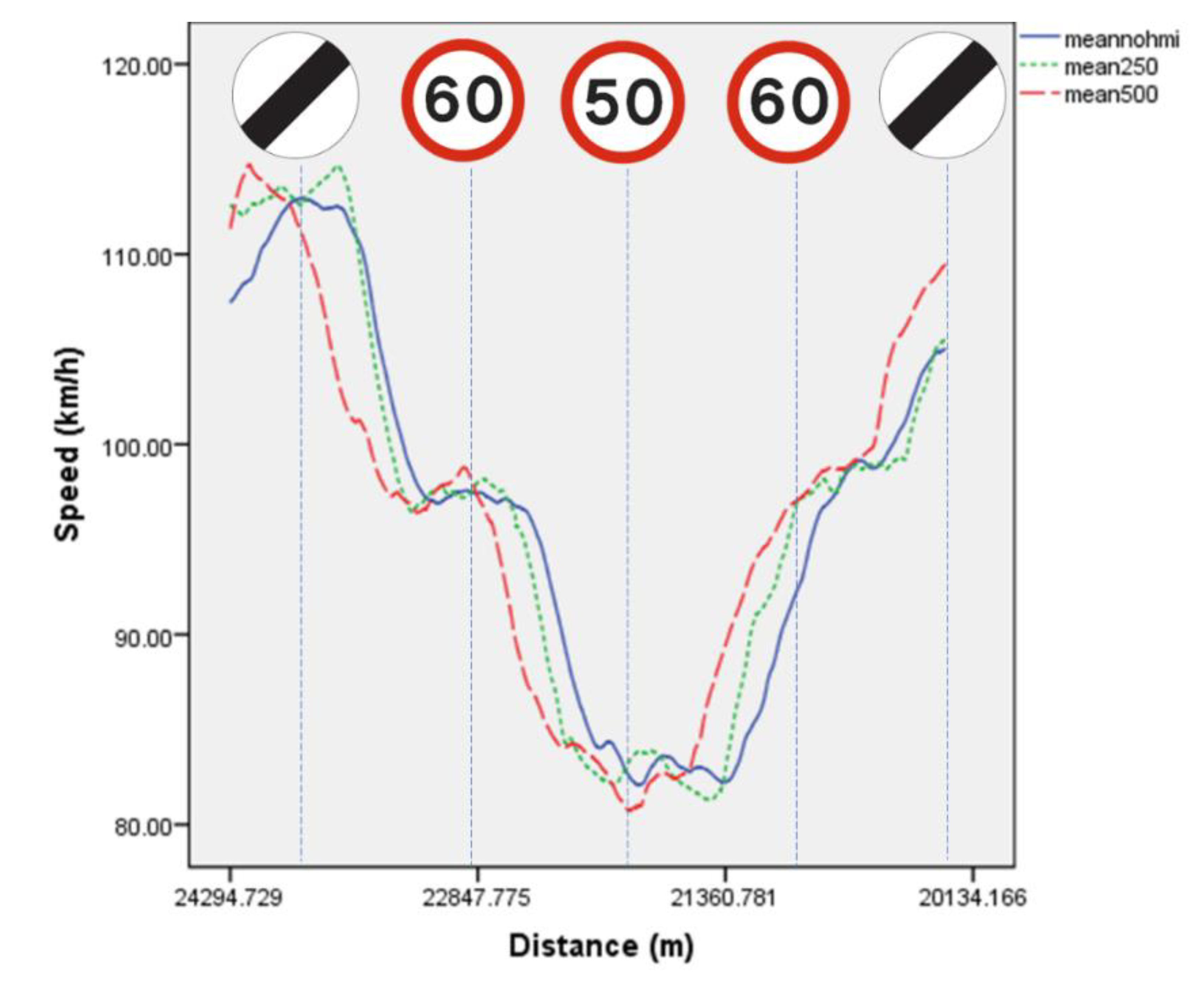
4.2. Speed Plots
4.3. Mean Speed Measured for 250 m and 500 m
4.3.1. Baseline Condition: noHMI
4.3.2. Experimental Conditions: HMI
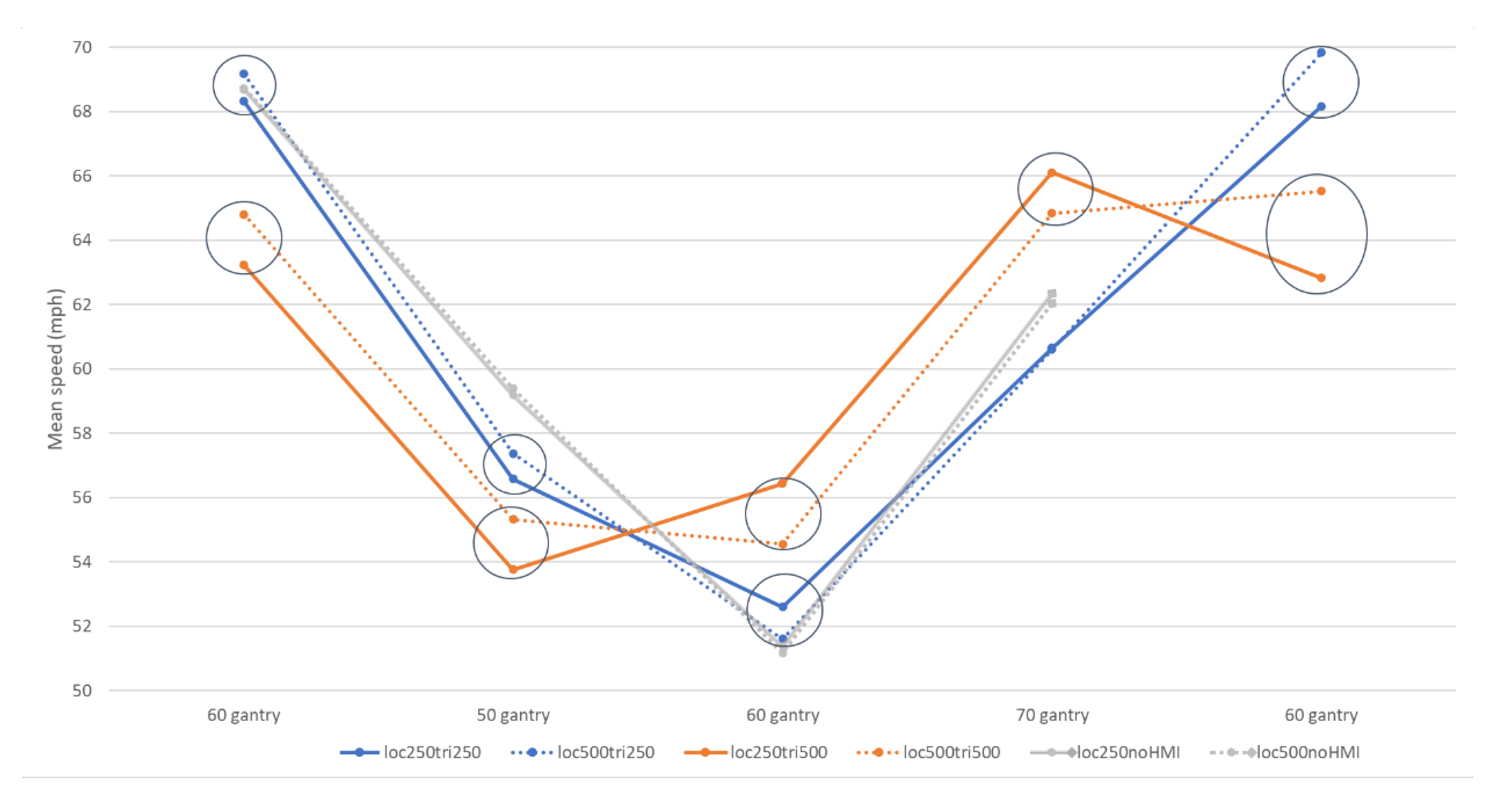
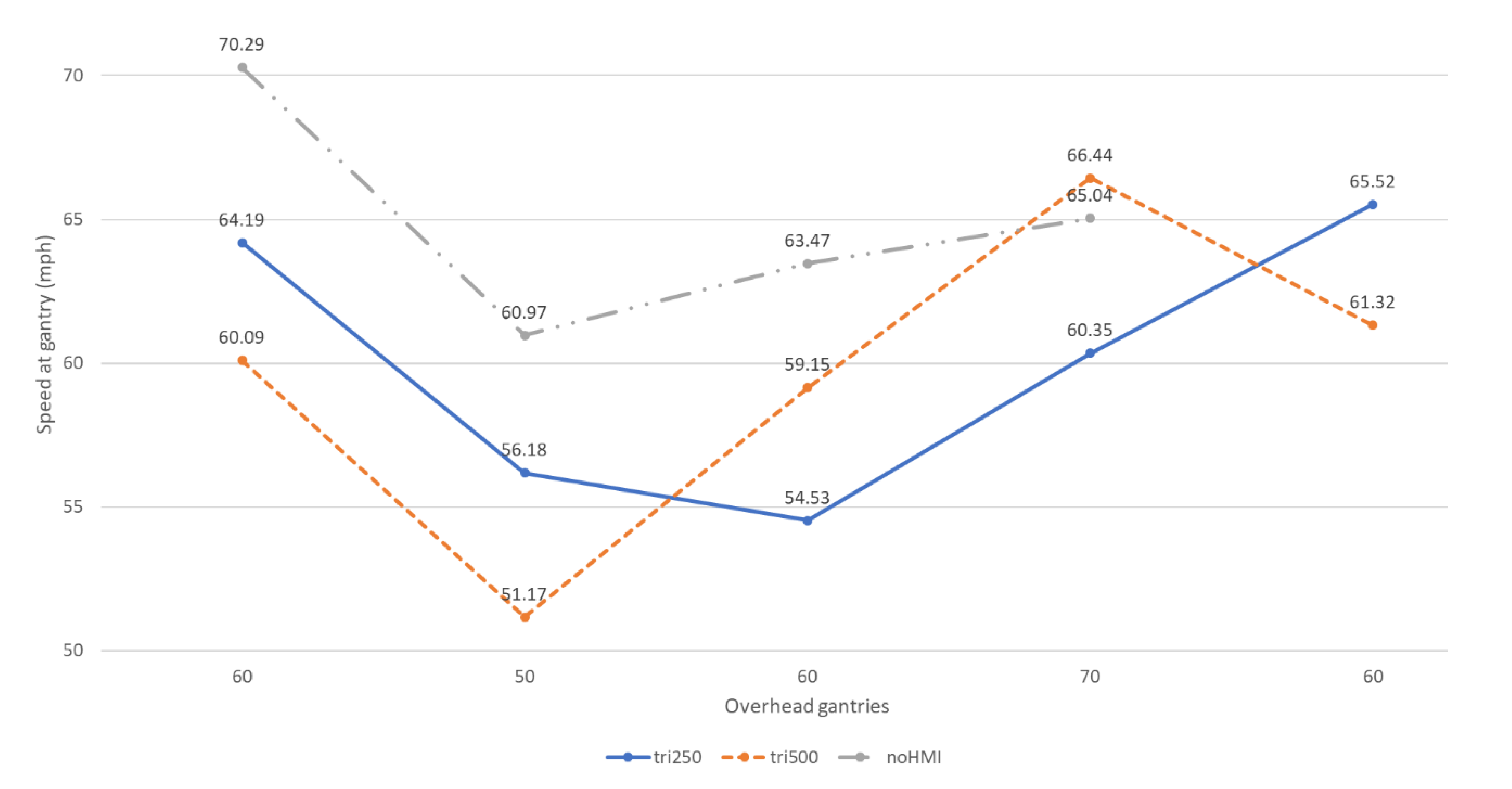
4.4. Speed at Gantry
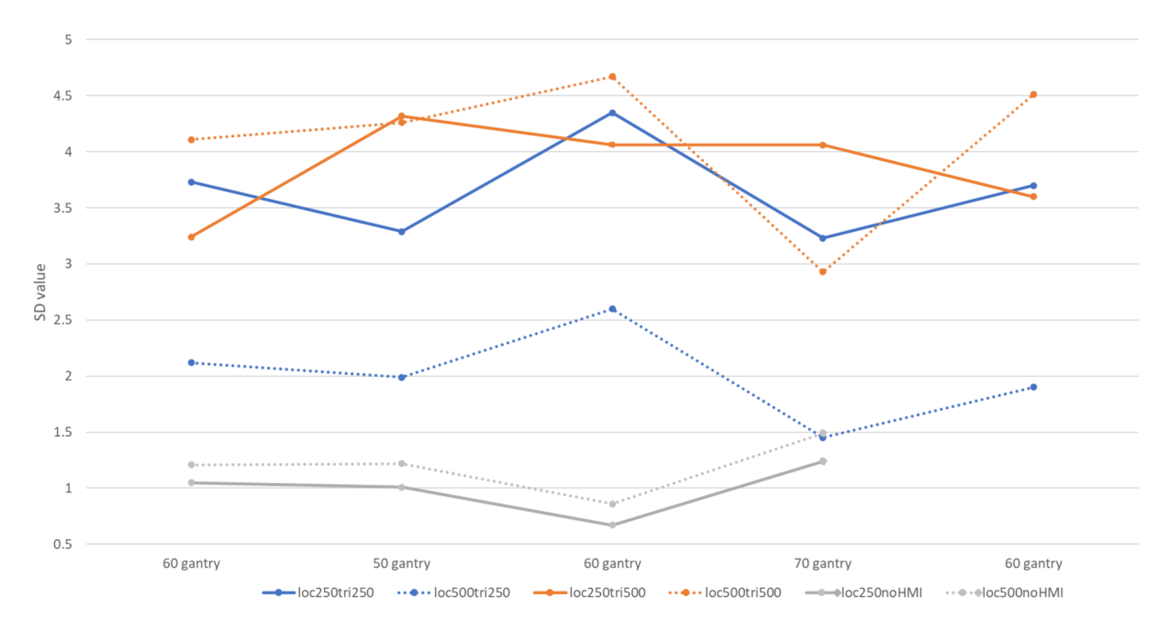
4.5. Speed Homogeneity
4.5.1. Baseline Condition: noHMI
4.5.2. Experimental Conditions: HMI
5. Discussion
6. Conclusions
Author Contributions
Funding
Institutional Review Board Statement
Informed Consent Statement
Data Availability Statement
Acknowledgments
Conflicts of Interest
References
- Van Nes, N.; Brandenburg, S.; Twisk, D. Improving homogeneity by dynamic speed limit systems. Accid. Anal. Prev. 2010, 42, 944–952. [Google Scholar] [CrossRef] [PubMed]
- Hoogendoorn, R.; Harms, I.; Hoogendoorn, S.; Brookhuis, K. Dynamic maximum speed limits: Perception, mental workload, and compliance. Transp. Res. Rec. J. Transp. Res. Board 2012, 2321, 46–54. [Google Scholar] [CrossRef]
- Chang, C.-Y.; Li, C.-C. Visual and operational impacts of variable speed limit signs on bus drivers on freeways using driving simulator. In Proceedings of the 3rd IEEE Asia-Pacific Services Computing Conference (APSCC 2008), Yilan, Taiwan, 9–12 December 2008; pp. 1453–1458. [Google Scholar] [CrossRef]
- Harms, I.M.; Brookhuis, K.A. Dynamic traffic management on a familiar road: Failing to detect changes in variable speed limits. Transp. Res. Part F Traffic Psychol. Behav. 2016, 38, 37–46. [Google Scholar] [CrossRef] [Green Version]
- Lee, C.; Abdel-Aty, M. Testing effects of warning messages and variable speed limits on driver behavior using driving simulator. Transp. Res. Rec. 2008, 2069, 55–64. [Google Scholar] [CrossRef]
- Hellinga, B.; Mandelzys, M. Impact of driver compliance on the safety and operational impacts of freeway variable speed limit systems. J. Transp. Eng. 2011, 137, 260–268. [Google Scholar] [CrossRef]
- Lehtonen, E.; Malhotra, N.; Starkey, N.J.; Charlton, S.G. Speedometer monitoring when driving with a speed warning system. Eur. Transp. Res. Rev. 2020, 12, 16. [Google Scholar] [CrossRef]
- Jamson, S. Would those who need ISA, use it? Investigating the relationship between drivers’ speed choice and their use of a voluntary ISA system. Transp. Res. Part F Traffic Psychol. Behav. 2006, 9, 195–206. [Google Scholar] [CrossRef] [Green Version]
- Lai, F.; Carsten, O. What benefit does Intelligent Speed Adaptation deliver: A close examination of its effect on vehicle speeds. Accid. Anal. Prev. 2012, 48, 4–9. [Google Scholar] [CrossRef] [PubMed]
- Whitmire, J., II; Morgan, J.F.; Oron-Gilad, T.; Hancock, P.A. The effect of in-vehicle warning systems on speed compliance in work zones. Transp. Res. Part F Traffic Psychol. Behav. 2011, 14, 331–340. [Google Scholar] [CrossRef]
- Endsley, M.R. Toward a theory of situation awareness in dynamic systems. Hum. Factors J. Hum. Factors Ergon. Soc. 1995, 37, 32–64. [Google Scholar] [CrossRef]
- Highways Agency. Highways Agency Policy for the Use of Variable Signs and Signals (VSS) Devices. Interim Advice Note 162/12. 2012. Available online: http://www.standardsforhighways.co.uk/ha/standards/ghost/ians/pdfs/ian162.pdf (accessed on 7 July 2022).
- Highways England. Traffic Signs Manual Chapter 1 Introduction; 2018; Crown: London, UK; ISBN 9780115536014. Available online: https://assets.publishing.service.gov.uk/government/uploads/system/uploads/attachment_data/file/771873/traffic-signs-manual-chapter-1.pdf (accessed on 7 July 2022).
- ISO/TS 16951:2004; Road Vehicles—Ergonomic Aspects of Transport Information and Control Systems (TICS)—Procedures for Determining Priority of on-board Messages Presented to Drivers. International Organization for Standardization: Geneva, Switzerland, 2004.
- Jerome, C.; Monk, C.; Campbell, J. Driver Vehicle Interface Design Assistance for Vehicle-to-Vehicle Technology Applications. In Proceedings of the 24th International Technical Conference on the Enhanced Safety of Vehicles (ESV), Gothenburg, Sweden, 8–11 June 2015. No. 15–0452. [Google Scholar]
- Brooke, J. Sus: A ‘quick and dirty’ usability scale. Usability Eval. Ind. 1996, 189, 4–7. [Google Scholar]
- Van der Laan, J.D.; Heino, A.; De Waard, D. A simple procedure for the assessment of acceptance of advanced transport telematics. Transp. Res. Part C Emerg. Technol. 1997, 5, 1–10. [Google Scholar] [CrossRef]
- Bangor, A.; Kortum, P.; Miller, J. Determining what individual SUS scores mean: Adding an adjective rating scale. J. Usability Stud. 2009, 4, 114–123. [Google Scholar]
- Speiran, J.; Shakshuki, E. Emergency Electronic Brake Lights for the Smartphone VANET. Procedia Comput. Sci. 2022, 203, 51–60. [Google Scholar] [CrossRef]
- Starkey, N.J.; Charlton, S.G.; Malhotra, N.; Lehtonen, E. Drivers’ response to speed warnings provided by a smart phone app. Transp. Res. Part C Emerg. Technol. 2020, 110, 209–221. [Google Scholar] [CrossRef]
- Ali, Y.; Sharma, A.; Haque, M.M.; Zheng, Z.; Saifuzzaman, M. The impact of the connected environment on driving behavior and safety: A driving simulator study. Accid. Anal. Prev. 2020, 144, 105643. [Google Scholar] [CrossRef] [PubMed]
- Warner, H.W.; Åberg, L. The long-term effects of an ISA speed-warning device on drivers’ speeding behaviour. Transp. Res. Part F Traffic Psychol. Behav. 2008, 11, 96–107. [Google Scholar] [CrossRef]
- Orne, M.T. Demand characteristics and the concept of quasi-controls. In Artifacts in Behavioral Research: Robert Rosenthal and Ralph L. Rosnow’s Classic Books; Oxford University Press: Oxford, UK, 2009; Volume 110, pp. 110–137. [Google Scholar]
- Silvano, A.P. Impacts of Speed Limits and Information Systems on Speed Choice from a Safety Perspective. Doctoral dissertation, KTH Royal Institute of Technology, Stockholm, Sweden, 2013. [Google Scholar]


| Within Subjects Factor | ||
|---|---|---|
| No HMI | ||
| HMI | ||
| Between subjects factor | trig250 m (10) | trig500 m (10) |
| Gantry | F | df | p Value | ηp2 | Distance to Gantry Measurement | Mean * | SD * |
|---|---|---|---|---|---|---|---|
| 70 mph (113 km/h) | 2.95 | 1, 19 | 0.10 | 0.13 | 250 m | 99.83 | 6.80 |
| 500 m | 99.16 | 6.36 | |||||
| 60 mph (97 km/h) | 0.75 | 1, 19 | 0.75 | 0.01 | 250 m | 110.52 | 4.89 |
| 500 m | 110.61 | 4.51 | |||||
| 50 mph (80 km/h) | 0.97 | 1, 19 | 0.34 | 0.05 | 250 m | 95.23 | 3.62 |
| 500 m | 95.56 | 3.72 | |||||
| 60 mph (97 km/h) | 1.78 | 1, 19 | 0.20 | 0.09 | 250 m | 82.65 | 5.06 |
| 500 m | 82.33 | 4.86 | |||||
| 70 mph (113 km/h) | 1.70 | 1, 19 | 0.21 | 0.08 | 250 m | 100.33 | 6.06 |
| 500 m | 99.83 | 5.73 |
| Gantry | Distance to Gantry Measurement | F | df | p Value | ηp2 | XP Condition | Mean * | SD * |
|---|---|---|---|---|---|---|---|---|
| 70 mph (113 km/h) | 250 m | 0.02 | 1, 18 | 0.883 | 0.00 | trig250 m | 99.59 | 8.12 |
| trig500 m | 100.07 | 5.61 | ||||||
| 500 m | 0.00 | 1, 18 | 0.974 | 0.00 | trig250 m | 99.12 | 7.71 | |
| trig500 m | 99.21 | 5.09 | ||||||
| 60 mph (97 km/h) | 250 m | 3.81 | 1, 18 | 0.067 | 0.18 | trig250 m | 108.52 | 5.59 |
| trig500 m | 112.52 | 3.23 | ||||||
| 500 m | 3.98 | 1, 18 | 0.061 | 0.18 | trig250 m | 108.74 | 5.37 | |
| trig500 m | 112.52 | 2.52 | ||||||
| 50 mph (80 km/h) | 250 m | 2.20 | 1, 18 | 0.156 | 0.11 | trig250 m | 94.07 | 4.79 |
| trig500 m | 96.39 | 1.32 | ||||||
| 500 m | 2.98 | 1, 18 | 0.102 | 0.14 | trig250 m | 94.19 | 4.68 | |
| trig500 m | 96.93 | 1.79 | ||||||
| 60 mph (97 km/h) | 250 m | 0.04 | 1, 18 | 0.841 | 0.00 | trig250 m | 82.42 | 5.54 |
| trig500 m | 82.89 | 4.82 | ||||||
| 500 m | 0.02 | 1, 18 | 0.895 | 0.00 | trig250 m | 82.48 | 5.93 | |
| trig500 m | 82.18 | 3.83 | ||||||
| 70 mph (113 km/h) | 250 m | 0.55 | 1, 18 | 0.469 | 0.03 | trig250 m | 101.34 | 6.25 |
| trig500 m | 99.32 | 6.01 | ||||||
| 500 m | 0.08 | 1, 18 | 0.778 | 0.01 | trig250 m | 100.20 | 6.43 | |
| trig500 m | 99.44 | 5.25 |
| Gantry | XP Condition | F | df | p Value | ηp2 | Distance to Gantry Measurement | Mean * | SD * |
|---|---|---|---|---|---|---|---|---|
| 60 mph (97 km/h) | trig250 m | 26.51 | 1, 9 | 0.001 | 0.75 | 250 m | 109.93 | 3.46 |
| 500 m | 101.31 | 3.04 | ||||||
| trig500 m | 23.56 | 1, 9 | 0.001 | 0.72 | 250 m | 101.74 | 5.77 | |
| 500 m | 104.28 | 5.33 | ||||||
| 50 mph (80 km/h) | trig250 m | 2.04 | 1, 9 | 0.187 | 0.19 | 250 m | 91.04 | 4.48 |
| 500 m | 91.04 | 4.48 | ||||||
| trig500 m | 19.11 | 1, 9 | 0.002 | 0.68 | 250 m | 86.51 | 4.58 | |
| 500 m | 89.03 | 3.27 | ||||||
| 60 mph (97 km/h) | trig250 m | 12.74 | 1, 9 | 0.006 | 0.59 | 250 m | 84.65 | 3.49 |
| 500 m | 83.04 | 3.10 | ||||||
| trig500 m | 13.97 | 1, 9 | 0.005 | 0.61 | 250 m | 90.82 | 5.80 | |
| 500 m | 87.78 | 5.00 | ||||||
| 70 mph (113 km/h) | trig250 m | 0.003 | 1, 9 | 0.956 | 0.00 | 250 m | 97.60 | 5.82 |
| 500 m | 97.54 | 6.22 | ||||||
| trig500 m | 9.25 | 1, 9 | 0.014 | 0.51 | 250 m | 106.37 | 7.70 | |
| 500 m | 104.32 | 6.69 | ||||||
| 60 mph (97 km/h) | trig250 m | 39.94 | 1, 9 | 0.000 | 0.82 | 250 m | 109.68 | 3.71 |
| 500 m | 112.38 | 2.98 | ||||||
| trig500 m | 45.36 | 1, 9 | 0.000 | 0.83 | 250 m | 101.10 | 5.19 | |
| 500 m | 105.44 | 5.02 |
| Gantry | XP Condition | F | df | p Value | ηp2 | Distance to Gantry Measurement | Mean * | SD * |
|---|---|---|---|---|---|---|---|---|
| 60 mph (97 km/h) | trig250 m | 14.8 | 1, 18 | 0.001 | 0.45 | 250 m | 109.93 | 3.46 |
| 500 m | 101.74 | 5.77 | ||||||
| trig500 m | 13.11 | 1, 18 | 0.002 | 0.42 | 250 m | 111.31 | 3.04 | |
| 500 m | 104.28 | 5.33 | ||||||
| 50 mph (80 km/h) | trig250 m | 5.0 | 1, 18 | 0.038 | 0.22 | 250 m | 91.04 | 4.48 |
| 500 m | 86.51 | 4.58 | ||||||
| trig500 m | 6.16 | 1, 18 | 0.023 | 0.26 | 250 m | 92.33 | 2.64 | |
| 500 m | 89.03 | 3.27 | ||||||
| 60 mph (97 km/h) | trig250 m | 8.29 | 1, 18 | 0.010 | 0.32 | 250 m | 84.65 | 3.49 |
| 500 m | 90.82 | 5.80 | ||||||
| trig500 m | 6.51 | 1, 18 | 0.020 | 0.27 | 250 m | 83.04 | 3.10 | |
| 500 m | 87.78 | 5.00 | ||||||
| 70 mph (113 km/h) | trig250 m | 8.26 | 1, 18 | 0.010 | 0.32 | 250 m | 97.60 | 5.82 |
| 500 m | 106.37 | 7.70 | ||||||
| trig500 m | 5.52 | 1, 18 | 0.030 | 0.24 | 250 m | 97.54 | 6.22 | |
| 500 m | 104.32 | 6.69 | ||||||
| 60 mph (97 km/h) | trig250 m | 18.10 | 1, 18 | 0.000 | 0.50 | 250 m | 109.68 | 3.71 |
| 500 m | 101.10 | 5.19 | ||||||
| trig500 m | 14.12 | 1, 18 | 0.001 | 0.44 | 250 m | 112.38 | 2.98 | |
| 500 m | 105.44 | 5.02 |
| Gantry | Distance to Gantry Measurement | F | df | p Value | ηp2 | XP Condition | Mean * | SD * |
|---|---|---|---|---|---|---|---|---|
| 60 mph (97 km/h) | 250 m | 0.838 | 1, 9 | 0.384 | 0.09 | noHMI | 108.53 | 5.60 |
| trig250 m | 109.93 | 3.46 | ||||||
| 500 m | 32.95 | 1, 9 | 0.136 | 0.23 | noHMI | 108.74 | 5.37 | |
| trig250 m | 111.31 | 3.04 | ||||||
| 50 mph (80 km/h) | 250 m | 2.87 | 1, 9 | 0.124 | 0.24 | noHMI | 94.07 | 4.79 |
| trig250 m | 91.04 | 4.48 | ||||||
| 500 m | 1.21 | 1, 9 | 0.299 | 0.12 | noHMI | 94.20 | 4.68 | |
| trig250 m | 92.33 | 2.64 | ||||||
| 60 mph (97 km/h) | 250 m | 1.41 | 1, 9 | 0.264 | 0.14 | noHMI | 82.42 | 5.54 |
| trig250 m | 84.65 | 3.49 | ||||||
| 500 m | 0.11 | 1, 9 | 0.751 | 0.01 | noHMI | 82.49 | 5.93 | |
| trig250 m | 83.04 | 3.10 | ||||||
| 70 mph (113 km/h) | 250 m | 1.83 | 1, 9 | 0.203 | 0.17 | noHMI | 101.35 | 6.25 |
| trig250 m | 97.60 | 5.82 | ||||||
| 500 m | 0.65 | 1, 9 | 0.442 | 0.07 | noHMI | 100.20 | 6.43 | |
| trig250 m | 97.53 | 6.22 |
| Gantry | Distance to Gantry Measurement | F | df | p Value | ηp2 | XP Condition | Mean * | SD * |
|---|---|---|---|---|---|---|---|---|
| 60 mph (97 km/h) | 250 m | 32.62 | 1, 9 | 0.000 | 0.78 | noHMI | 112.52 | 3.24 |
| trig500 m | 101.74 | 5.77 | ||||||
| 500 m | 18.85 | 1, 9 | 0.002 | 0.68 | noHMI | 112.49 | 2.53 | |
| trig500 m | 104.28 | 5.33 | ||||||
| 50 mph (80 km/h) | 250 m | 49.99 | 1, 9 | 0.000 | 0.85 | noHMI | 96.40 | 1.32 |
| trig500 m | 86.51 | 4.58 | ||||||
| 500 m | 48.41 | 1, 9 | 0.000 | 0.84 | noHMI | 96.93 | 1.79 | |
| trig500 m | 89.03 | 3.27 | ||||||
| 60 mph (97 km/h) | 250 m | 18.82 | 1, 9 | 0.002 | 0.68 | noHMI | 82.90 | 4.82 |
| trig500 m | 90.82 | 5.79 | ||||||
| 500 m | 25.64 | 1, 9 | 0.001 | 0.74 | noHMI | 82.19 | 3.83 | |
| trig500 m | 87.78 | 4.99 | ||||||
| 70 mph (113 km/h) | 250 m | 10.13 | 1, 9 | 0.011 | 0.53 | noHMI | 99.32 | 6.01 |
| trig500 m | 106.37 | 7.70 | ||||||
| 500 m | 8.35 | 1, 9 | 0.018 | 0.48 | noHMI | 99.45 | 5.26 | |
| trig500 m | 104.32 | 6.69 |
| Gantry | F | df | p Value | ηp2 | XP Condition | Mean * | SD * |
|---|---|---|---|---|---|---|---|
| 60 mph (97 km/h) | 11.66 | 1, 18 | 0.003 | 0.39 | trig250 m | 103.27 | 5.09 |
| trig500 m | 96.69 | 3.34 | |||||
| 50 mph (80 km/h) | 5.36 | 1, 18 | 0.033 | 0.23 | trig250 m | 90.40 | 10.11 |
| trig500 m | 82.33 | 4.41 | |||||
| 60 mph (97 km/h) | 10.84 | 1, 18 | 0.004 | 0.38 | trig250 m | 87.75 | 4.55 |
| trig500 m | 95.17 | 5.50 | |||||
| 70 mph (113 km/h) | 9.87 | 1, 18 | 0.006 | 0.35 | trig250 m | 97.77 | 5.04 |
| trig500 m | 106.90 | 8.47 | |||||
| 60 mph (97 km/h) | 7.39 | 1, 18 | 0.14 | 0.29 | trig250 m | 105.43 | 6.50 |
| trig500 m | 98.66 | 4.44 |
| Gantry | HMI trigger Distance to Gantry | F | df | p Value | ηp2 | XP Condition | Mean * | SD * |
|---|---|---|---|---|---|---|---|---|
| 60 mph (97 km/h) | 250 m | 12.09 | 1, 9 | 0.007 | 0.57 | noHMI | 113.37 | 6.84 |
| trig250 m | 103.27 | 5.09 | ||||||
| 500 m | 395.02 | 1, 9 | 0.000 | 0.98 | noHMI | 114.81 | 2.26 | |
| trig500 m | 96.70 | 3.34 | ||||||
| 50 mph (80 km/h) | 250 m | 3.24 | 1, 9 | 0.105 | 0.26 | noHMI | 96.39 | 5.65 |
| trig250 m | 90.4 | 10.10 | ||||||
| 500 m | 70.38 | 1, 9 | 0.000 | 0.89 | noHMI | 99.71 | 3.61 | |
| trig500 m | 82.33 | 4.41 | ||||||
| 60 mph (97 km/h) | 250 m | 69.42 | 1, 9 | 0.000 | 0.89 | noHMI | 99.65 | 2.41 |
| trig250 m | 87.74 | 4.55 | ||||||
| 500 m | 32.96 | 1, 9 | 0.000 | 0.79 | noHMI | 104.61 | 2.25 | |
| trig500 m | 95.17 | 5.50 | ||||||
| 70 mph (113 km/h) | 250 m | 17.64 | 1, 9 | 0.002 | 0.66 | noHMI | 104.82 | 3.30 |
| trig250 m | 97.11 | 5.04 | ||||||
| 500 m | 1.29 | 1, 9 | 0.289 | 0.12 | noHMI | 104.49 | 5.50 | |
| trig500 m | 106.90 | 8.47 |
| Gantry | F | df | p Value | ηp2 | Distance to Gantry Measurement | Mean * | SD * |
|---|---|---|---|---|---|---|---|
| 70 mph (113 km/h) | 2.25 | 1, 19 | 0.15 | 0.11 | 250 m | 2.68 | 1.39 |
| 500 m | 2.99 | 1.45 | |||||
| 60 mph (97 km/h) | 1.01 | 1, 19 | 0.33 | 0.05 | 250 m | 1.69 | 0.82 |
| 500 m | 1.95 | 0.73 | |||||
| 50 mph (80 km/h) | 2.16 | 1, 19 | 0.16 | 0.10 | 250 m | 1.63 | 0.73 |
| 500 m | 1.96 | 0.70 | |||||
| 60 mph (97 km/h) | 1.53 | 1, 19 | 0.23 | 0.07 | 250 m | 1.07 | 0.79 |
| 500 m | 1.38 | 1.18 | |||||
| 70 mph (113 km/h) | 1.85 | 1, 19 | 0.19 | 0.09 | 250 m | 1.99 | 1.27 |
| 500 m | 2.39 | 1.36 |
| Gantry | Distance to Gantry Measurement | F | df | p Value | ηp2 | XP Condition | Mean * | SD * |
|---|---|---|---|---|---|---|---|---|
| 70 mph (113 km/h) | 250 m | 0.33 | 1, 18 | 0.574 | 0.02 | trig250 m | 2.86 | 1.53 |
| trig500 m | 2.50 | 1.30 | ||||||
| 500 m | 0.26 | 1, 18 | 0.615 | 0.01 | trig250 m | 3.17 | 1.81 | |
| trig500 m | 2.83 | 1.03 | ||||||
| 60 mph (97 km/h) | 250 m | 0.01 | 1, 18 | 0.913 | 0.00 | trig250 m | 1.67 | 0.77 |
| trig500 m | 1.71 | 0.92 | ||||||
| 500 m | 1.69 | 1, 18 | 0.211 | 0.09 | trig250 m | 2.16 | 0.84 | |
| trig500 m | 1.74 | 0.57 | ||||||
| 50 mph (80 km/h) | 250 m | 0.17 | 1, 18 | 0.687 | 0.01 | trig250 m | 1.70 | 0.91 |
| trig500 m | 1.57 | 0.54 | ||||||
| 500 m | .03 | 1, 18 | 0.862 | 0.00 | trig250 m | 1.93 | 0.32 | |
| trig500 m | 1.99 | 0.97 | ||||||
| 60 mph (97 km/h) | 250 m | 1.42 | 1, 18 | 0.250 | 0.07 | trig250 m | 1.28 | 0.88 |
| trig500 m | 0.86 | 0.68 | ||||||
| 500 m | 0.30 | 1, 18 | 0.594 | 0.02 | trig250 m | 1.53 | 1.25 | |
| trig500 m | 1.24 | 1.14 | ||||||
| 70 mph (113 km/h) | 250 m | 0.88 | 1, 18 | 0.360 | 0.05 | trig250 m | 2.25 | 1.30 |
| trig500 m | 1.72 | 1.26 | ||||||
| t500 m | .17 | 1, 18 | 0.690 | 0.01 | trig250 m | 2.52 | 1.65 | |
| trig500 m | 2.26 | 1.06 |
| Gantry | XP Condition | F | df | p Value | ηp2 | Distance to Gantry Measurement | Mean * | SD * |
|---|---|---|---|---|---|---|---|---|
| 60 mph (97 km/h) | trig250 m | 12.33 | 1, 18 | 0.002 | 0.41 | 250 m | 3.73 | 1.10 |
| 500 m | 2.12 | 0.93 | ||||||
| trig500 m | 3.77 | 1, 18 | 0.081 | 0.16 | 250 m | 3.24 | 0.95 | |
| 500 m | 4.11 | 1.14 | ||||||
| 50 mph (80 km/h) | trig250 m | 8.51 | 1, 18 | 0.004 | 0.36 | 250 m | 3.29 | 1.04 |
| 500 m | 1.99 | 0.71 | ||||||
| trig500 m | 0.02 | 1, 18 | 0.923 | 0.00 | 250 m | 4.32 | 1.50 | |
| 500 m | 4.26 | 1.48 | ||||||
| 60 mph (97 km/h) | trig250 m | 15.21 | 1, 18 | 0.025 | 0.25 | 250 m | 4.35 | 1.97 |
| 500 m | 2.60 | 1.10 | ||||||
| trig500 m | 1.88 | 1, 18 | 0.51 | 0.02 | 250 m | 4.06 | 1.63 | |
| 500 m | 4.67 | 2.38 | ||||||
| 70 mph (113 km/h) | trig250 m | 15.86 | 1, 18 | 0.007 | 0.34 | 250 m | 3.23 | 1.58 |
| 500 m | 1.45 | 0.98 | ||||||
| trig500 m | 6.33 | 1, 18 | 0.196 | 0.09 | 250 m | 4.06 | 1.88 | |
| 500 m | 2.93 | 1.86 | ||||||
| 60 mph (97 km/h) | trig250 m | 16.13 | 1, 18 | 0.018 | 0.28 | 250 m | 3.70 | 1.87 |
| 500 m | 1.90 | 1.11 | ||||||
| trig500 m | 4.15 | 1, 18 | 0.333 | 0.05 | 250 m | 3.60 | 1.83 | |
| 500 m | 4.51 | 2.24 |
| Gantry | Distance to Gantry Measurement | F | df | p Value | ηp2 | XP Condition | Mean SD Score * |
|---|---|---|---|---|---|---|---|
| 60 mph (97 km/h) | 250 m | 34.58 | 1, 9 | 0.000 | 0.79 | noHMI | 1.67 |
| trig250 m | 3.73 | ||||||
| 500 m | 29.18 | 1, 9 | 0.000 | 0.76 | noHMI | 1.74 | |
| trig250 m | 4.11 | ||||||
| 50 mph (80 km/h) | 250 m | 11.77 | 1, 9 | 0.008 | 0.57 | noHMI | 1.70 |
| trig250 m | 3.29 | ||||||
| 500 m | 22.17 | 1, 9 | 0.001 | 0.71 | noHMI | 1.93 | |
| trig250 m | 4.32 | ||||||
| 60 mph (97 km/h) | 250 m | 27.13 | 1, 9 | 0.001 | 0.75 | noHMI | 1.28 |
| trig250 m | 4.35 | ||||||
| 500 m | 31.90 | 1, 9 | 0.005 | 0.61 | noHMI | 1.53 | |
| trig250 m | 4.06 | ||||||
| 70 mph (113 km/h) | 250 m | 2.01 | 1, 9 | 0.19 | 0.18 | noHMI | 2.25 |
| trig250 m | 3.23 | ||||||
| 500 m | 3.24 | 1, 9 | 0.11 | 0.27 | noHMI | 2.52 | |
| trig250 m | 4.06 |
| Gantry | Distance to Gantry Measurement | F | df | p Value | ηp2 | XP Condition | Mean SD Score * |
|---|---|---|---|---|---|---|---|
| 60 mph (97 km/h) | 250 m | 0.83 | 1, 9 | 0.387 | 0.08 | noHMI | 1.72 |
| trig500 m | 2.12 | ||||||
| 500 m | 29.18 | 1, 9 | 0.000 | 0.76 | noHMI | 1.74 | |
| trig500 m | 4.11 | ||||||
| 50 mph (80 km/h) | 250 m | 2.43 | 1, 9 | 0.153 | 0.21 | noHMI | 1.57 |
| trig500 m | 1.99 | ||||||
| 500 m | 16.13 | 1, 9 | 0.003 | 0.64 | noHMI | 1.99 | |
| trig500 m | 4.26 | ||||||
| 60 mph (97 km/h) | 250 m | 12.17 | 1, 9 | 0.007 | 0.58 | noHMI | 0.86 |
| trig500 m | 2.60 | ||||||
| 500 m | 10.26 | 1, 9 | 0.011 | 0.53 | noHMI | 1.24 | |
| trig500 m | 4.67 | ||||||
| 70 mph (113 km/h) | 250 m | 0.26 | 1, 9 | 0.622 | 0.03 | noHMI | 1.71 |
| trig500 m | 1.45 | ||||||
| 500 m | 0.71 | 1, 9 | 0.419 | 0.07 | noHMI | 2.27 | |
| trig500 m | 2.93 |
Disclaimer/Publisher’s Note: The statements, opinions and data contained in all publications are solely those of the individual author(s) and contributor(s) and not of MDPI and/or the editor(s). MDPI and/or the editor(s) disclaim responsibility for any injury to people or property resulting from any ideas, methods, instructions or products referred to in the content. |
© 2022 by the authors. Licensee MDPI, Basel, Switzerland. This article is an open access article distributed under the terms and conditions of the Creative Commons Attribution (CC BY) license (https://creativecommons.org/licenses/by/4.0/).
Share and Cite
Payre, W.; Diels, C. Driving Behaviour and Usability: Should In-Vehicle Speed Limit Warnings Be Paired with Overhead Gantry? Future Transp. 2023, 3, 1-22. https://doi.org/10.3390/futuretransp3010001
Payre W, Diels C. Driving Behaviour and Usability: Should In-Vehicle Speed Limit Warnings Be Paired with Overhead Gantry? Future Transportation. 2023; 3(1):1-22. https://doi.org/10.3390/futuretransp3010001
Chicago/Turabian StylePayre, William, and Cyriel Diels. 2023. "Driving Behaviour and Usability: Should In-Vehicle Speed Limit Warnings Be Paired with Overhead Gantry?" Future Transportation 3, no. 1: 1-22. https://doi.org/10.3390/futuretransp3010001