Using Machine Learning to Classify Human Fetal Health and Analyze Feature Importance

Abstract

The reduction of childhood mortality is an ongoing struggle and a commonly used factor in determining progress in the medical field. The under-5 mortality number is around 5 million around the world, with many of the deaths being preventable. In light of this issue, cardiotocograms (CTGs) have emerged as a leading tool to determine fetal health. By using ultrasound pulses and reading the responses, CTGs help healthcare professionals assess the overall health of the fetus to determine the risk of child mortality. However, interpreting the results of the CTGs is time consuming and inefficient, especially in underdeveloped areas where an expert obstetrician is hard to come by. Using a support vector machine (SVM) and oversampling, this paper proposes a model that classifies fetal health with an accuracy of 99.59%. To further explain the CTG measurements, an algorithm based off of RISE (Randomized Input Sampling for Explanation of Black-box Models) was created, called Feature Alteration for explanation of Black Box Models (FAB). The findings of this novel algorithm were compared to SHapley Additive exPlanations (SHAP) and Local Interpretable Model Agnostic Explanations (LIME). Overall, this technology allows doctors and medical professionals to classify fetal health with high accuracy and determine which features were most influential in the process.

1. Introduction

Infant mortality has been a continuing issue for many decades in healthcare systems around the world. Although we have developed instruments that can assess many aspects of fetal health, reading and interpreting CTG data is not always possible in regions that lack an expert obstetrician. Even in places with access to medical professionals, diagnosing a fetus one at a time based on CTG measurements can be extremely time consuming and generally inefficient. However, using machine learning models, fetal health classifications can be made without the presence of obstetricians and in a much more timely manner. These models can be highly accurate in their predictions, making them viable solutions to the problem of fetal health, while this solution works theoretically, there were still some major issues with implementing machine learning models. First of all, these models provide no help in identifying the problem with the fetus if it is deemed pathological. Obstetricians will not be able to properly treat their patients if they do not know why the fetus is in danger. Another issue is that patients may not trust a machine to give them a diagnosis, especially when there is no way for them to see how the model arrived at a particular classification.

The most efficient way to solve these problems is to implement an explainable model, which is a model that can not only predict results with high accuracy, but can also explain how it arrived at the decision to scientists implementing the model. With this knowledge, obstetricians can inform their patients what the exact metric is that is abnormal, and also be able to better treat their patient based on the abnormality. For example, if the model was to predict a pathological case for a fetus, it would also be able to show that the reason behind the prediction was a low number of uterine contractions per second. Using this knowledge, a doctor can relay this to their patient, advising rest and hydration, while in more severe cases, administer drugs such as Oxytocin to help bring levels back to normal [1].

In order to achieve this type of high performing yet explainable model, three different models were implemented: an extreme gradient boost classifier, a light gradient boost classifier, and a support vector classifier. A high accuracy was obtained with all three, meaning that the explainable portion was ready to be added. Building on previous success with high accuracy models, the models used previously tested SHAP [2] and LIME [3] values to rank feature importance. Both sets of metrics were then compared, with a considerable overlap in important features. With these two new metrics, the novel algorithms were able to accurately predict which measurements from the cardiotocogram were the most influential in the prediction.

In order to more accurately explain the model and have more methods to rely on, Feature Altering for explanations of Black box models (FAB), was created. This algorithm was inspired by RISE [4], a metric that was previously used in image classification problems. FAB analyzes feature importance through a unique technique of removing individual features and checking the accuracy. The new algorithm was tested with all three of the high performing models, which added yet another metric to measure the feature importance in the models.

Overall, the proposed algorithm uses random sampling as the backbone structure. This algorithm, combined with the SHAP [5] and LIME values, is a great way to provide insight into the predictions of the black box model. This is extremely important for healthcare providers when dealing with patients, and it adds a level of trust that might not have been there when patients were obtaining results from a machine without knowing how the prediction was formed. This can be a valuable addition to predicting fetal health in the medical field, along with FAB; the algorithm is not only extremely helpful in this situation, but also in any other machine learning problems where feature importance is required from tabular data.

2. Literature Review

Fetal health has been an important branch of research in public health, and the classification of fetal health has been conducted in various experiments. Most research was focused on classifying the fetal health with a high accuracy. Many different methods were used to achieve this high accuracy, such as filtering-based feature selection [6], classifying based on association(CBA) [7], and classifying using only selected features [8]. This problem has also been tackled using different types of models, such as deep learning neural networks [9], k-nearest neighbor [10], and even blended models [11]. Generally, a 99% accuracy was obtained, with high precision and recall [12]. This accuracy is very high and meets the threshold for real life applicability; however, many of the models used were black box models that lacked an explainable component. An explainable model can be beneficial to improving the ease of use of the technology, especially in cases where certain features can be detrimental in the overall prediction [13]. Furthermore, explainable models are highly important for healthcare professionals because the previous models only return classifications, which can lead to questions being raised by patients over how the model came to that prediction. The proposed model aims to fix this issue by adding explainability to a high performing classifier.

3. Methods and Materials

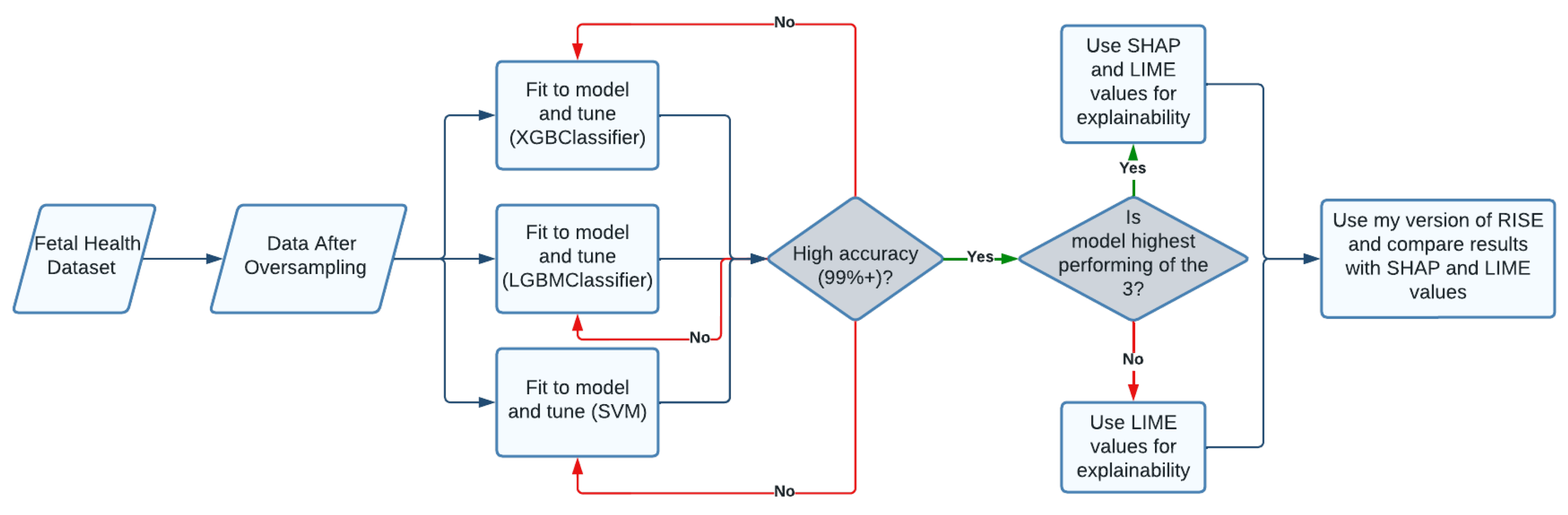
The overarching goal of this research is to create an effective way of classifying fetuses by risk of death using cardiotocogram data. To be able to do this in a clinical setting, it is imperative that the model used has a high accuracy of over 99.5%. The next step would then be to make the black box model explainable. This ensures that doctors understand which features play an important role in the diagnosis of the fetus, and is useful to healthcare providers in determining why exactly the fetus is at risk. This allows more generalized doctors to better serve their patients.

Figure 1 is a visual designed to briefly go over the research steps taken, and show how the data was used to eventually come up with an effective model.

3.1. Data Set

The first step to creating the machine learning model was understanding and manipulating the data so that it could be used. The data was obtained from a paper that collected CTG measurements, reported the data, and created a machine learning model called Sisporto to classify the data [14]. The measurements were collected by the authors of the paper from all around the world, making it ideal for training the model. The data set contained 2126 records of measurements extracted from Cardiotocogram exams, which were then annotated by three expert obstetricians into 3 classes: class 1 refers to normal health, class 2 indicates a possible risk to the fetus, and class 3 is pathological. For each instance, the obstetricians agreed on 1 classification. For each examination by the CTG, 21 features were recorded. These features measured many trends in fetal heart rate such as variations, accelerations and decelerations, and histogram values of the heart rates. Along with that, uterine contractions in the mother and movements by the fetus were also measured and recorded.

Table 1. Below is the list of all of the features in the data set along with their corresponding feature number, which is used various times throughout this research in order to address different features.

Feature #	Feature	Feature #	Feature
0	Baseline Value	11	Histogram Width
1	Accelerations	12	Histogram Min
2	Fetal Movement	13	Histogram Max
3	Uterine Contractions	14	Histogram Number of Peaks
4	Light Decelerations	15	Histogram Number of Zeroes
5	Severe Decelerations	16	Histogram Mode
6	Prolonged Decelerations	17	Histogram Mean
7	Abnormal Short Term Variability	18	Histogram Median
8	Mean Value of Short Term Variability	19	Histogram Variance
9	Percentage of Time With Abnormal Long Term Variability	20	Histogram Tendency
10	Mean Value of Long Term Variability

shows these features.

3.2. Exploratory Analysis of Features

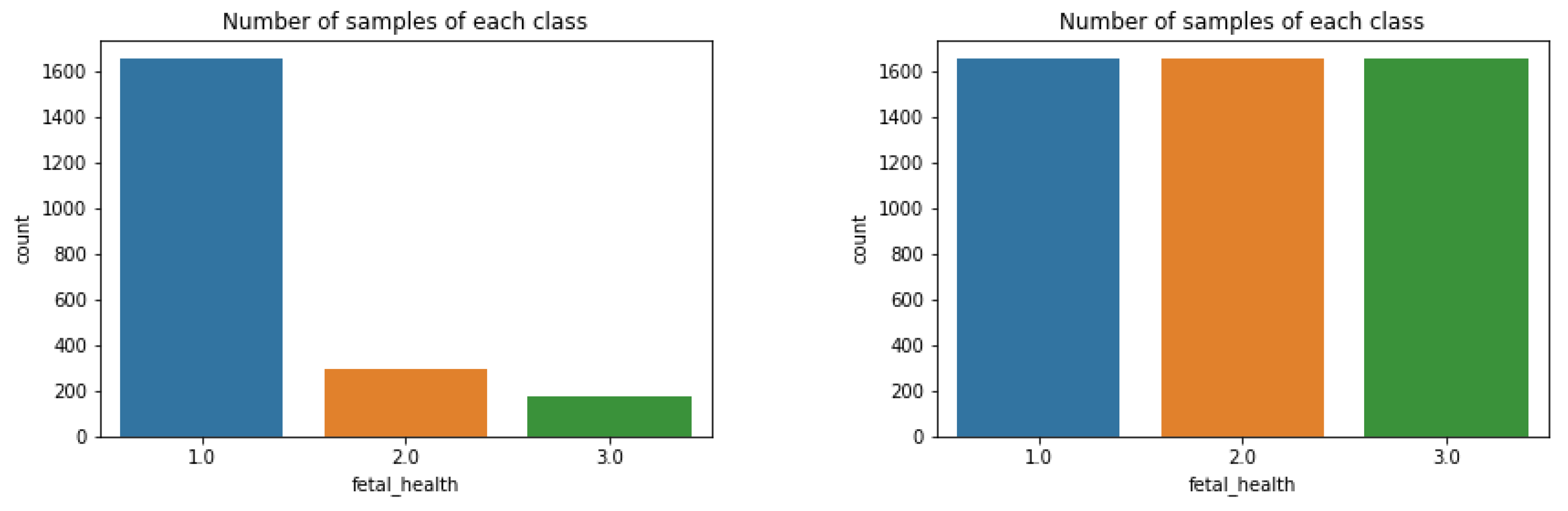
As shown in Figure 2, there was a severe imbalance in the number of occurrences of each label.

This is a result of the observational imbalances when sampling abnormalities; in our case, it is much more common for premature babies to be healthy than to be pathological. A skewed class distribution can be detrimental to the performance of machine learning models because of the tendency of the models to pick the higher probability classes incorrectly over the correct class. Previously, oversampling has been effective on this data set [15]. In our case, oversampling worked by creating duplicate sets of data for classes 2 and 3. In order to test the optimal training oversampling split, different ratios were tested. As shown in

Table 2. This table shows the performance of the training data at different levels of oversampling. The percentages represent the number of data points in the minority classes relative to the majority class, which is normal fetal health.

	Acc	Bal Acc	F1	ROC AUC
25%	0.919	0.897	0.920	0.965
50%	0.964	0.961	0.964	0.988
75%	0.986	0.987	0.986	0.998
100%	0.995	0.995	0.995	0.998

, there were 4 different ratios of oversampling tested, each with a different percentage of minority class samples. Optimal results were achieved with 100% oversampling, so this ratio was used.

The classes were duplicated until all three classes had the same number of instances, as shown in Figure 2. The graph on the left shows the number instances of each label before oversampling, while the right shows the counts after oversampling. All of the features were also used in the models because of the variability in each measurement. This meant that each feature was important in the health of the fetus.

After each class contained the same number of instances, the data was ready to be fit to a model. In order to achieve the highest performance possible in the classification, three different models (XGBoost, LightGBM, and SVM) were fitted to the data and tuned to achieve the highest possible results. XGBoost models have been proven to work with high accuracy in the past [16], which is why it was implemented. The second algorithm, LightGBM, was implemented in order to solve some potential drawbacks of the XGBoost classifier. LightGBM works quicker and more efficiently with larger datasets while still using the same model fitting process. In real life applications of the model, it would be ideal for the model to perform quickly with larger amounts of data. Lastly, a Support Vector Machine was implemented due to high classification rates in the past [17], along with the need for implementing a different type of machine learning model instead of only using gradient boosting.

3.3. Algorithms

The first model used was a special version of a gradient boosting model. It is an ensemble learning algorithm similar to random forest algorithms. Gradient Boosting models work by training ensembles of shallow decision trees; with each iteration, the model uses the residual error of the tree to help fit the ensuing decision tree. After many of these trees are built, the final prediction comes from a weighted sum. An Extreme Gradient Boost model differs in that the trees are built in parallel to each other instead of sequentially. This helps increase performance while also decreasing the time necessary to fit data to a model. This model is very popular in the scientific world, and tends to work well with a variety of problems.

The next model implemented was LightGBM, which stands for light gradient boosting machine. Similar to the previous XGBClassifer, this model is another ensemble gradient boosting algorithm. However, the main difference between the two is in the way the decision trees are made. In the XGBoost model, the decision trees grow by level, meaning that every new tree made would differ from the previous tree in that the new tree would have an extra level of leaves under it. On the other hand, LightGBM grows by individual nodes and leaves. Instead of a whole new level being added for every iteration, only some leaves are added. This is useful because LightGBM can be extremely accurate while also reducing the run time, hence the name. One potential problem with LightGBM is overfitting, but this can be combated with the use of the max depth parameter, which ensures that no individual tree has too many nodes.

After using 2 algorithms based on gradient boosting, the next step was to try a different type of model. A support vector machine (SVM) is useful because of how it is efficient and tends to work well with relatively smaller sets of data, such as the fetal health data. An SVM is a classification model that works by plotting data points on a plane. On a simple data set with 2 features, this would be a 2-dimensional plane, with all the data plotted using the x and y-axis for each feature. On this plane, the Support Vector Classifier (SVC) would then create a hyperplane, or a decision boundary, in between the 2 classes of data, and use that in determining which class the data goes in. As we increase features, the data is plotted in more and more dimensions, and the hyperplane also becomes more dimensions. For our data, the hyperplane is created in a way where 3 different classes are formed: one class is formed for normal fetuses, one is formed for suspect cases, and the last is formed for pathological cases. From here, the test data is then classified into each group based on where it is located relative to the hyperplane.

3.4. Model Evaluation Metrics

To measure the results of the model on our test data, four different metrics were used. The first metric is accuracy, which returns the percentage of correctly classified cases. The next column shows balanced accuracy, which is measured by calculating the average of the recall obtained by each class. Another metric used was F1 scores. In simple terms, this is the harmonic mean of precision and recall. An F1 score is calculated for each class, and the score is then averaged to obtain a singular score. Lastly, ROC AUC (Area Under the Receiver Operating Characteristic Curve) was used, which is a metric that calculates the area under an ROC curve. This curve is plotted using the fraction of the sensitivity divided by one minus the specificity at various different thresholds. Overall, this value determines how good the model is at distinguishing between classes. All 4 of these metrics work best for measuring success in different parts of the model, so the goal of the proposed models is to perform well under all 4 metrics. This would show that the models are successful and accurate in various different types of metrics.

3.5. Model Evaluation and Selection

The 3 models were trained using a 75:25 train test split. As per the name, 75% of the data were used to train the model, while the remaining 25% were used to test the model. This is a very common split to use when testing models, and the relatively higher percent of training data is beneficial in increasing the accuracy of the models used. For each model, the default parameters were initially used when fitting the data. From there, the parameters were changed one at a time in order to find the optimum values. In order to measure the performance, all of the metrics explained above were calculated. The results were displayed in tables in order to easily identify which parameters allowed the model to classify the CTG data with the highest success. Base models were first tested on the data in order to make sure that unnecessary tuning was not performed, along with confirming the fact that the data contained trends that could be analyzed to classify the data accurately. Once baseline models were tested, they were tuned to achieve the highest performance. Then, the models were compared to each other. Overall, all 4 metrics were used to make a decision on the best model.

3.5.1. XGBClassifier

The XGBClassifier was able to classify the data with a 96% accuracy, using default parameters. Although this number is quite high, a 4% rate of error is far too high for any practical use, especially when dealing with life and death. The first parameter tuned was the n_estimators parameter. This parameter determines the number of "trees" in the forest. In other words, it regulates the number of iterations used in total. Increasing the number of estimators generally increases performance on the training data, and more closely fits the model to the data. However, having too many estimators can increase the time it takes to fit the model to the data; in most cases, performance either decreases or stays the same after a certain point. Using a for loop, different values of n_estimators were tested, ranging from 50 to 300 with increments of 50.

Table 3. Tuning the n_estimators parameter on the XGBClassifier model. Performance plateaus at 250 estimators. The accuracy is denoted as “Acc”. The balanced accuracy is denoted as “Bal Acc”. The Receiver Operating Characteristics Area Under Curve (ROC AUC) is also presented.

	Acc	Bal Acc	F1	ROC AUC
50	0.938	0.937	0.938	0.989
100	0.954	0.953	0.954	0.992
150	0.964	0.964	0.964	0.994
200	0.965	0.964	0.965	0.995
250	0.975	0.974	0.974	0.996
300	0.975	0.974	0.974	0.996

shows the results of all the different values of n_estimators.

The best performance came with an n_estimators value of 250, so that was the value that was used when tuning the next parameters.

Table 4. Tuning the learning rate parameter on the XGBClassifier model. There is a positive relationship between learning rate and performance, with a learning rate of 1 being the highest performing. The accuracy is denoted as “Acc”. The balanced accuracy is denoted as “Bal Acc”. The Receiver Operating Characteristics Area Under Curve (ROC AUC) is also presented.

	Acc	Bal Acc	F1	ROC AUC
0.000001	0.721	0.722	0.719	0.875
0.000010	0.721	0.722	0.719	0.875
0.000100	0.721	0.722	0.719	0.875
0.001000	0.735	0.738	0.737	0.877
0.100000	0.925	0.924	0.926	0.986
1.000000	0.975	0.974	0.974	0.996

showed the results of tuning the learning rate parameter. Learning rate is a weighting factor applied to the new trees in a model. In other words, the learning rate controls how quickly the model adapts and fits to the data. A learning rate too low for the given data can result in the model not being able to fit to the data and the model needing a lot of estimators. On the other hand, a learning rate too high can result in overfitting, which would cause poor performance on new data. According to Table 4, a learning rate of 1 yields the highest performance.

Using the XGBClassifier model with 250 estimators and a learning rate of 1, the max depth parameter was tuned. This parameter regulates the longest distance from root to leaf. We do not want our tree to have too many leaves because this can result in overfitting and it can take a lot of time. It is also not ideal to have a max depth that is too small because the classifications will not be as accurate.

Table 5. Tuning the max depth of the XGBClassifier model. Using the accuracy metrics and the f1 score, a max depth of 15 is optimal. The accuracy is denoted as “Acc”. The balanced accuracy is denoted as “Bal Acc”. The Receiver Operating Characteristics Area Under Curve (ROC AUC) is also presented.

	Acc	Bal Acc	F1	ROC AUC
1	0.975	0.974	0.974	0.996
5	0.986	0.986	0.986	0.998
10	0.986	0.986	0.986	0.998
15	0.987	0.987	0.987	0.998
20	0.987	0.987	0.987	0.998
25	0.987	0.987	0.987	0.998
32	0.987	0.987	0.987	0.998

shows different max depths and the metrics used to measure performance. A max depth of 15 seems to be optimal because anything bigger seems to yield the same results. We do not want to waste time with a larger max depth when it is not necessary, which is why a max depth of 15 is optimal.

After tuning the XGBClassifer with 3 different parameters, the model was able to classify the fetal health with an accuracy of around 98.79%, with each label being classified correctly above 98% of the time. This is much better than before, which shows how important tuning a model can be to the performance.

3.5.2. LGBMClassifier

When the LGBMClassifier model was first fit to the fetal health data, a 95% accuracy was achieved using the default parameters. Since tuning the XGBoost model yielded a higher accuracy, the same strategy was implemented to try and maximize the performance of the LightGBM. The first parameter tuned was n_estimators. As shown in

Table 6. Tuning the n_estimators parameter for the LGBMClassifier. There seems to be a positive linear relationship between performance and number of estimators. The accuracy is denoted as “Acc”. The balanced accuracy is denoted as “Bal Acc”. The Receiver Operating Characteristics Area Under Curve (ROC AUC) is also presented.

	Acc	Bal Acc	F1	ROC AUC
50	0.941	0.940	0.941	0.990
100	0.955	0.955	0.955	0.993
150	0.961	0.960	0.961	0.994
200	0.969	0.968	0.969	0.995
250	0.974	0.973	0.974	0.995
300	0.975	0.975	0.975	0.995

, as the number of estimators went up, the performance increased. However, the increase seemed to be slowing down as the model approached 300 estimators. Going over 300 estimators could easily cause overfitting and it is costly computationally. As a result, it is not advised in practice generally.

After deciding on using 300 estimators, the next parameter to tune was learning rate. As mentioned previously, learning rate controls how quickly the model adapts to the problem.

Table 7. Tuning the learning rate of the LGBMClassifier model. Using accuracy and F1 score, a learning rate of 1 is the best for this dataset. However, using AUC, a learning rate of 0.1 is optimal. The accuracy is denoted as “Acc”. The balanced accuracy is denoted as “Bal Acc”. The Receiver Operating Characteristics Area Under Curve (ROC AUC) is also presented.

	Acc	Bal Acc	F1	ROC AUC
0.000001	0.322	0.333	0.157	0.987
0.000010	0.553	0.567	0.460	0.987
0.000100	0.927	0.926	0.927	0.987
0.001000	0.943	0.942	0.943	0.992
0.010000	0.980	0.980	0.980	0.998
0.100000	0.991	0.991	0.991	0.999
1.000000	0.992	0.992	0.992	0.998

shows that a learning rate of 1 produces the highest accuracy and F1 score, and has only a slightly lower ROC area under curve. Since the learning rate is a multiplier, it is illogical to increase it above 1.

The final parameter tuned was max depth. This parameter is especially important to the LightGBM because this particular model works by adding leaves, and if this was not regulated, then the forest could become too complex and become inefficient.

Table 8. Tuning the max depth of the LGBMClassifier. A max depth of 5 results in the highest value of all 4 metrics. The accuracy is denoted as “Acc”. The balanced accuracy is denoted as “Bal Acc”. The Receiver Operating Characteristics Area Under Curve (ROC AUC) is also presented.

	Acc	Bal Acc	F1	ROC AUC
1	0.927	0.926	0.927	0.987
5	0.991	0.991	0.991	0.999
10	0.991	0.991	0.991	0.999
15	0.991	0.991	0.991	0.999
20	0.991	0.991	0.991	0.999
25	0.991	0.991	0.991	0.999
32	0.991	0.991	0.991	0.999

shows that there is a peak in accuracy and balanced accuracy with a max depth of 5.

After tuning all 3 parameters, the final LighGBM was able to achieve a 99.19% accuracy, with each label being classified correctly above 98% of the time. This was higher than the XGBoost model, with a rate of error less than 1%. One possible reason for this increase in performance was the leaf wise split instead of the level wise split, which fit the data to the model well. Along with that, to prevent overfitting, we used a relatively low max depth, which led to a higher performing and quicker model than the XGBoost Model.

3.5.3. SVM

With SVM models, the 2 main parameters that are most influential to model performance are the C parameter and the gamma parameter. Generally, these 2 parameters are altered in order to achieve better results [18]. The support vector classifier (SVC) was first tuned with the C parameter. This parameter determines how rigid you want your hyperplane to be with regard to outliers in data. With a high C, outliers can influence the location of the hyperplane and end up causing a high misclassification rate. On the other hand, a low C can possibly ignore data points that are on the border of classes. If the testing data happens to have more points like this, using a low C will cause a high misclassification rate. To find the optimal value, many different parameters of C ranging from 0.01 to 1000, ascending by powers of 10, were tested.

Table 9. Tuning the C parameter in the SVC model. The highest metrics seem to be obtained with a higher C of 1000. The accuracy is denoted as “Acc”. The balanced accuracy is denoted as “Bal Acc”. The Receiver Operating Characteristics Area Under Curve (ROC AUC) is also presented.

	Acc	Bal Acc	F1	ROC AUC
0.01	0.664	0.667	0.670	0.861
0.10	0.803	0.803	0.805	0.918
1.00	0.819	0.818	0.820	0.936
10.00	0.838	0.838	0.840	0.957
100.00	0.878	0.877	0.879	0.971
1000.00	0.918	0.917	0.918	0.978

shows that the higher values of C seemed to work better, with a C of 1000 being the most accurate in all metrics.

The next parameter tuned was the gamma parameter. This parameter regulates how closely the hyperplane is fit to the classes. For example, a higher gamma value would result in the plane being very close to the boundaries of the training data, basically creating an area for the class only where the training data is. A high gamma value would overfit the data by fitting the decision boundaries only around the training data. On the other hand, a lower gamma value would create a more broader hyperplane and not confine the boundaries as close to the test data. This means that the decision boundaries would not be as complex. This can be beneficial, but it can also lead to underfitting if the gamma is too low, which is why it is important to find the right balance.

Table 10. Tuning the gamma parameter in the SVC model. The accuracy and F1 score plateau at a gamma of 1, while the ROC AUC reaches a peak at a gamma of 0.1. The accuracy is denoted as “Acc”. The balanced accuracy is denoted as “Bal Acc”. The Receiver Operating Characteristics Area Under Curve (ROC AUC) is also presented.

	Acc	Bal Acc	F1	ROC AUC
0.001	0.977	0.976	0.977	0.993
0.010	0.989	0.989	0.989	0.998
0.100	0.995	0.995	0.995	0.999
1.000	0.996	0.996	0.996	0.999
10.000	0.996	0.996	0.996	0.998
100.000	0.996	0.996	0.996	0.998

shows that a gamma of 1 produces the same accuracy as anything higher than that, meaning that a gamma of 1 is optimal. Furthermore, a gamma of 0.1 has the highest ROC AUC, but it is marginal.

Overall, using a C of 1000 and a gamma of 1, the accuracy of the model jumped to 99.59%, with each label being classified correctly over 99% of the time. This is extremely high, and the misclassification rate was just over 0.4%. This model has performed higher than both of the previous models, and with an accuracy this high, can be used in real life situations to predict fetal health around the world. In places where an expert health provider who can read cardiotocographs is rare, this model can predict the health of the fetus with an extremely high probability.

4. Results

After tuning, the proposed models achieved a 98.79% accuracy with the extreme gradient boost, a 99.19% accuracy with the light gradient boost, and a 99.59% accuracy with the support vector machine on our test data. All three of these are very accurate and quick models that can be used around the world in places where it is inefficient for an obstetrician to determine fetal health on a case by case basis. However, in order to further enhance the usability of the models, it is necessary to transform the algorithms from black box models to explainable models. Although there are trends that can be found in many of the features [19], it is time consuming and inefficient for a doctor to look through each feature for every new case and try to find abnormalities within each measurement. The 3 ways explainability has been implemented is through the use of SHapley Additive exPlanations (SHAP) values, Local Interpretable Model Agnostic Explanations (LIME), and a novel algorithm that works on tabular data. All of these methods serve primarily to determine which features from the data are most influential when making a prediction, and can be extremely beneficial to the public health field in allowing doctors and obstetricians to better help diagnose and treat specific problems that are causing suspect and pathological cases in fetuses.

4.1. SHAP

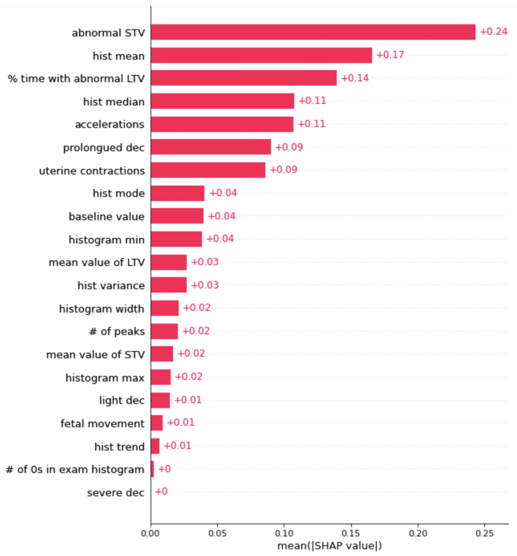
The first method used to explain the results of the model was the SHapley Additive exPlanations algorithm, or SHAP for short [20]. SHAP is a method based on game theory that is used to increase interpretability of the results returned by a machine learning model. This works through complex mathematical algorithms that assign numbers to each feature and either add or subtract from the number based on the feature’s overall contribution to the prediction made. This is performed for every iteration in the data set; at the end, the final number assigned to each feature represents its importance in the overall classification of the data. The reason this method was chosen over other explainability methods is its ability to provide a complete explanation between the global average and the model output for a particular explanation. Along with that, SHAP spends a lot more time than other algorithms in considering all possible predictions for an instance using all possible combinations of inputs. As a result, there is generally higher local accuracy. Figure 3 shows the SHAP graph for the most important features, ranked in order, for the XGBoost model.

The most important feature is short term variability (STV). STV is a measurement of the beat-to-beat variation in the fetal heart rate, and the CTG keeps track of the number of times the variation is abnormal in a fetus [21]. Another important feature worth noting is accelerations, which are abrupt increases in the baseline fetal heart rate of greater than 15 bpm for greater than 15 s. This feature is important because our LIME values also rank this feature high up on the list of the most important features. This claim is backed up by clinical studies as well, with accelerations tending to have a big role in the health of a fetus [22].

The next model to be explained was the light gradient boost model, shown in Figure 4. The graph itself was similar to the graph of the SHAP values for the extreme gradient boosting models, because they both use a similar process to arrive at a classification. The graph shows that abnormal STV is the most important feature, followed by histogram mean and percentage of time with long term variability. Prolonged decelerations and uterine contractions are also influential, surrounded by many different histogram measurements. Looking at both the SHAP graphs so far, there seems to be a trend of the same groups of features having the highest SHAP values, such as abnormal STV and histogram values.

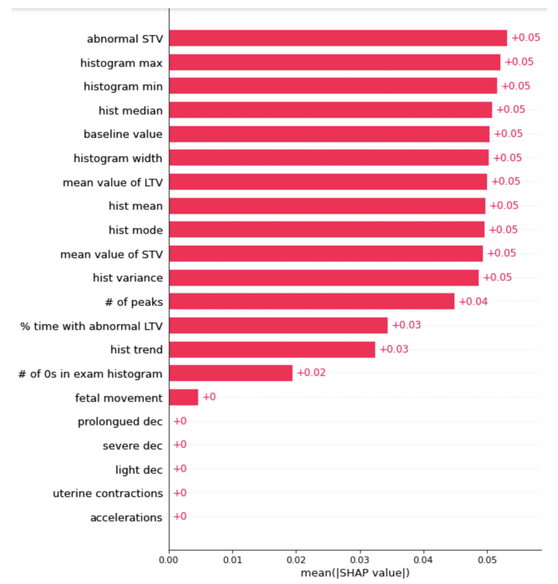
Lastly, the SHAP graph for the support vector machine is shown above in Figure 5. This graph shows that for our SVM, there were many different features that each played a relatively equal role in the classification of the data. From observing Figure 5, a similar result appeared: abnormal STV was one of the most influential features, followed by many of the histogram values. Abnormal STV, or abnormal short term variability, measures the percentage of time that the fetus had abnormal variability in heart rate from beat to beat, hence the short term aspect. The histogram values represent the baby’s heart rates that were measured, all plotted on a histogram. Histogram max and min were also important in the classification of the fetal health, along with many other features. Overall, the SVM model was very balanced in feature importance, which means that it is not too dependent on a singular feature when making predictions.

4.2. LIME

The next way to explain the models was to use Local Interpretable Model Agnostic Explanations, or LIME for short. LIME builds sparse linear models around each prediction to explain how the black box model works in that local vicinity. It takes one individual piece of data and creates new data based on the real one, only keeping some aspects of the feature distribution the same. The replicated data will differ from the original row of data in almost every way except for a couple of key similarities, such as individual measurements from one feature or the distribution of certain features. Then, the data is classified using the model given. By looking at the classification of the new data, we can tell which segments of the data were important in the overall classification. The main reason that LIME was chosen is because it is a quicker and more efficient way of explaining a model. It does not take a lot of time like SHAP does, and it generates a list of important features at the end. This is because while SHAP analyzes each individual prediction to gather results, LIME only selects one instance to replicate data from. These two algorithms complement each other nicely; when used together, they can provide a much more comprehensive explanation of the data.

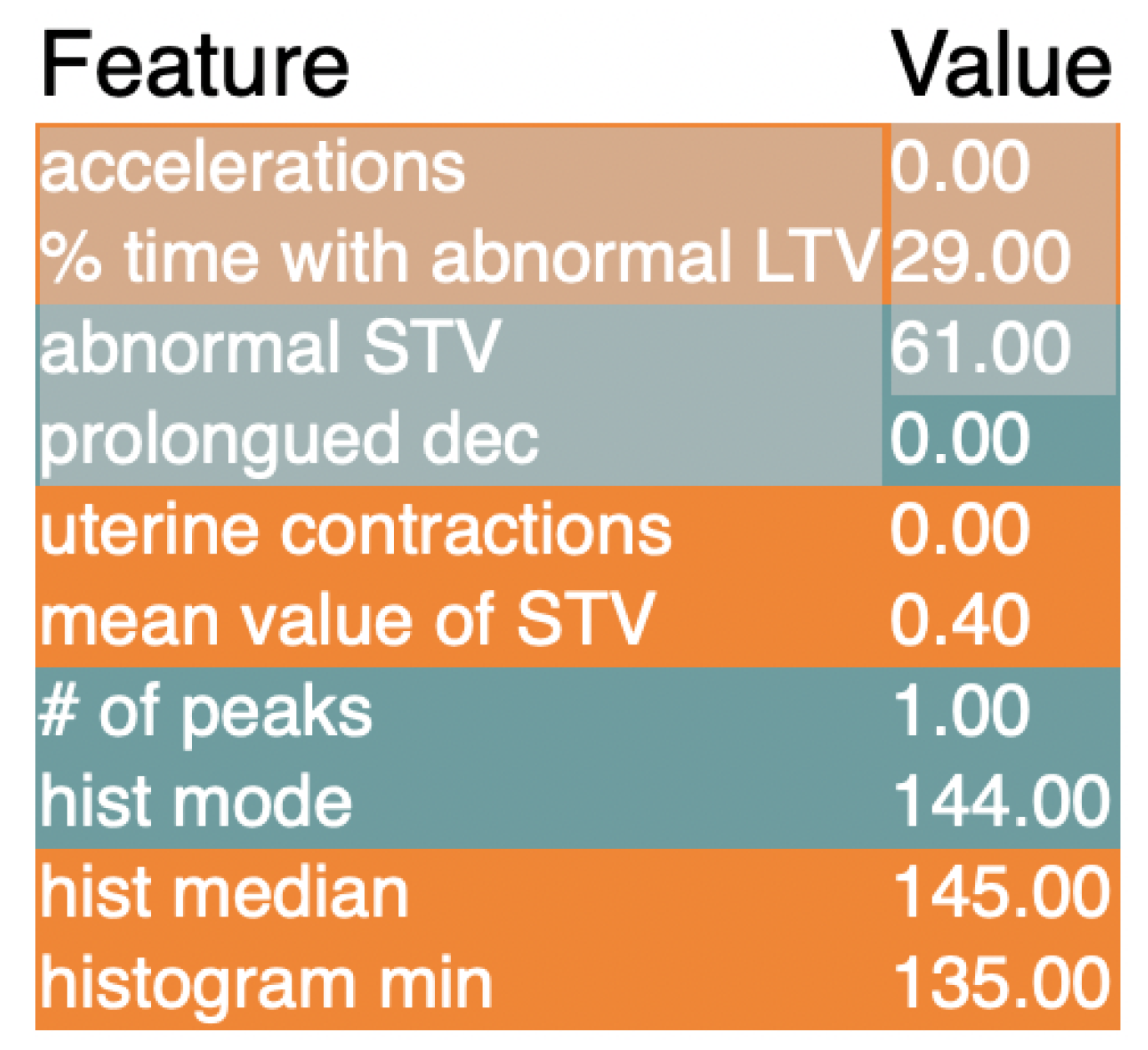
Figure 6 shows the LIME explanation for the XGBoost model. Just as with the SHAP values, accelerations are shown as a measurement that is extremely important to the model. Next up is the percentage of time with abnormal long term variation, which is a similar measurement to short term variability except for the duration of time. Abnormal short term variation is next up, which was also shown by SHAP as an important feature. Overall, many of the values marked as important by the SHAP algorithm were also marked as important using LIME.

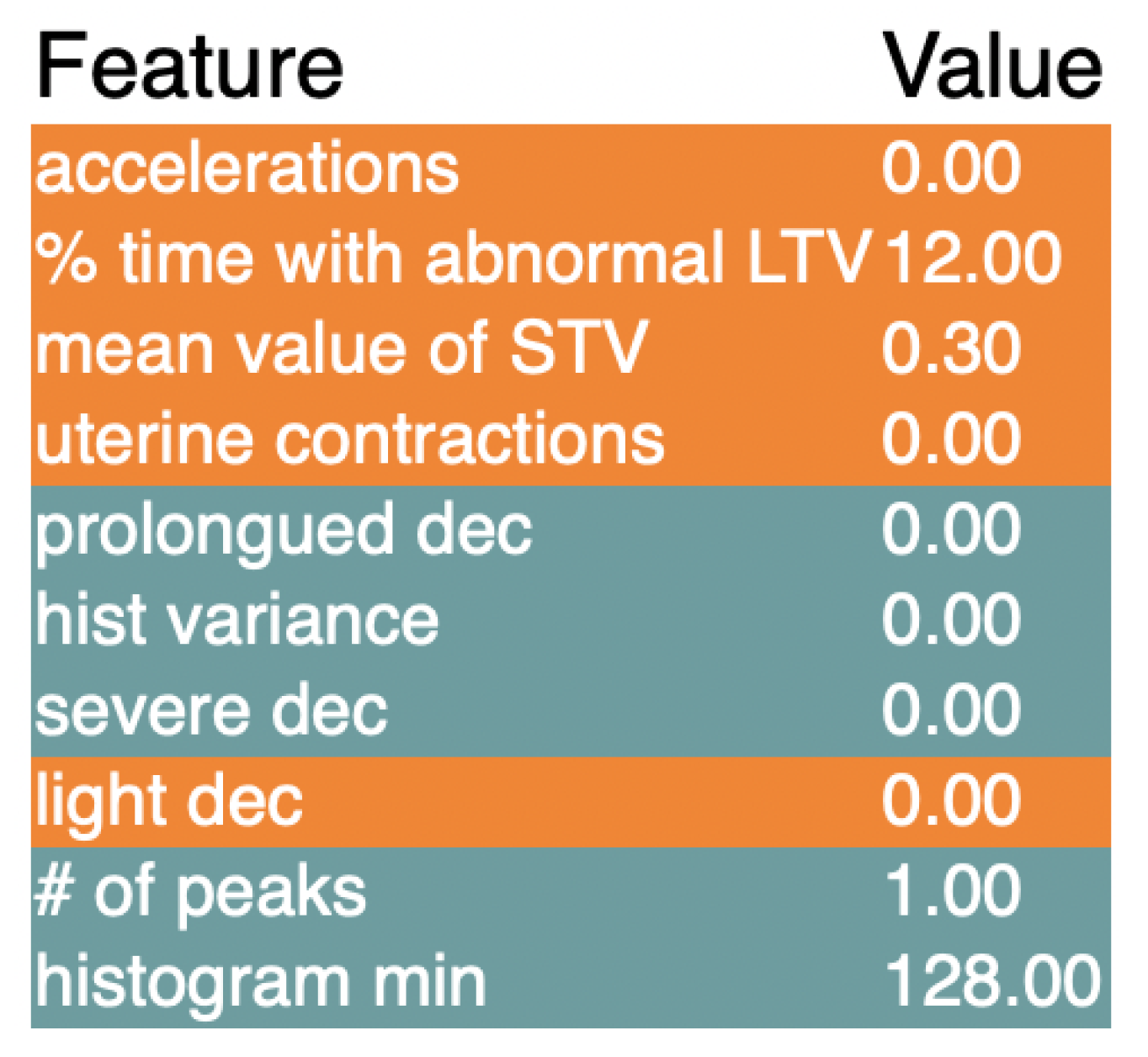
Figure 7 shows the results of LIME when used on the LGBM classifier. Again, accelerations seem to be the most important feature, followed by percentage of time with abnormal LTV. After that, mean value of STV and uterine contractions are also flagged as important, while a couple of deceleration metrics are also on the list. Decelerations are the opposite of accelerations, and occur when there are abrupt decreases in baseline fetal heart rate. Rounding out some of the most important features for the LightGBM are histogram values, similar to other models and the SHAP explanations.

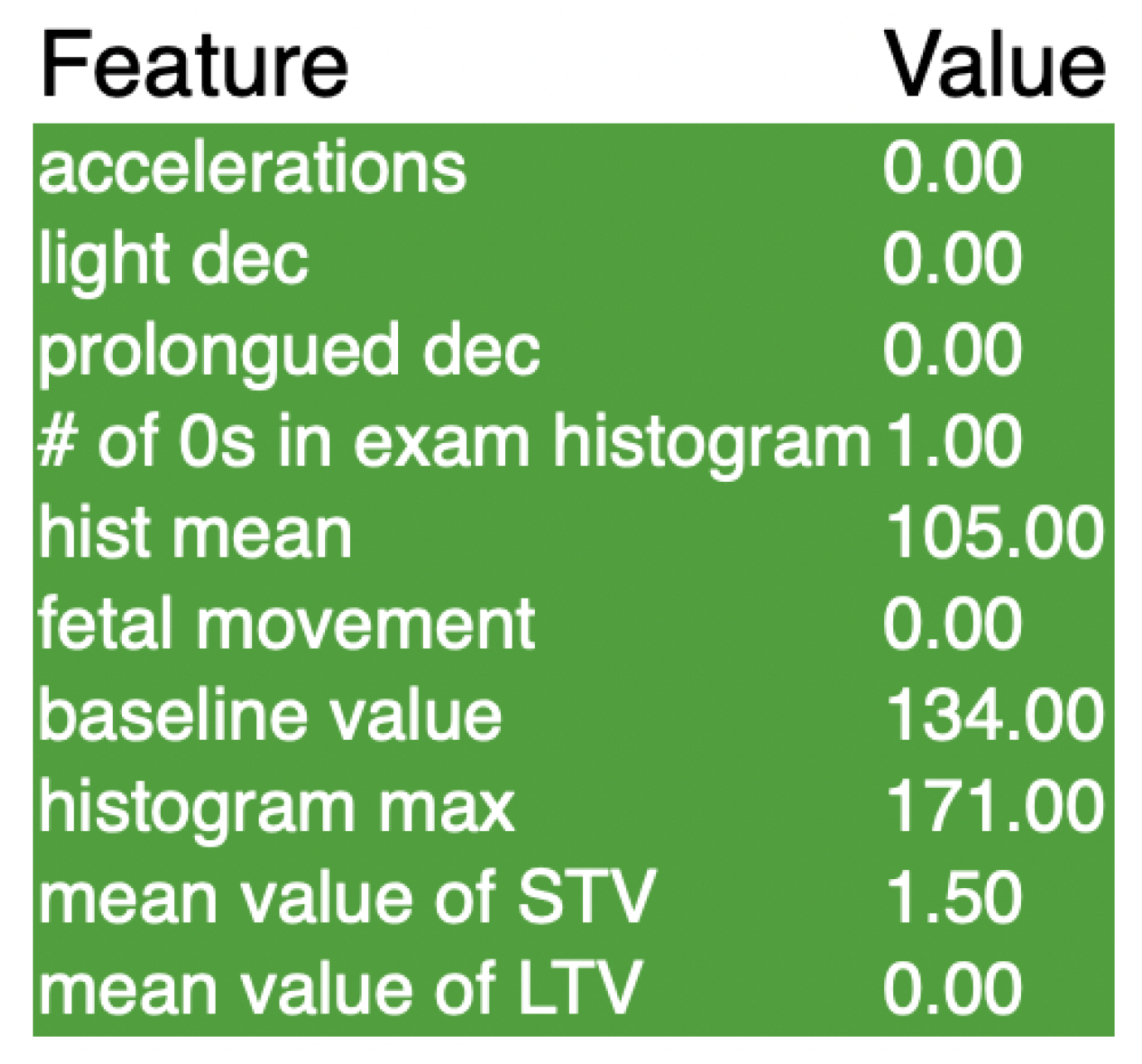
Lastly, Figure 8 shows the explanations for LIME when implemented on the SVM. Accelerations yet again top the chart as the most important feature in the classification, while decelerations take the next two spots. There are also a couple of histogram values in the list, similar to the previous LIME explanations. Overall, the lists for both the LIME and the SHAP values have been fairly consistent, and there are a group of key features that stand out as being extremely important to the classification in all three of the models. Using these two methods for explaining the models will certainly be beneficial for clinical use, and will allow healthcare providers to specify their diagnosis and treatment specifically towards the detected problem.

4.3. Feature Altering for Explanations of Black Box Models (FAB)

Although the SHAP and LIME values were both extremely beneficial in understanding the black box models better, Feature Altering for explanations of Black box models (FAB) was implemented in order to rank feature importance using a new approach. This method is modeled from RISE, which was an already existing way of explaining black box models. However, this method was only compatible with images, and was not viable to use with tabular data. FAB builds off of RISE by using the same logic to explain models that use tabular data. The reason that FAB was implemented was to provide a different approach from that of SHAP and LIME. The differences between these algorithms rely mainly in the way the data is manipulated. With SHAP, the data is not manipulated at all, and simply observed to see weights in predictions. With LIME, the data is manipulated by creating new datasets based on a single measurement. Finally, with FAB, the data is manipulated by removing a feature and not altering anything else. This algorithm also produced similar results to both SHAP and LIME in all of our models, confirming the most important features in classification.

The already existing RISE is used to determine which parts of an image were most important in classification of it. This is performed by dividing the picture into many small boxes, and then removing one box from the total image. Then, the model is tested on the modified image and returns the classification, along with how confident it is in the classification. If the model classifies correctly with high confidence, then we can be sure that the piece that was removed was not very important in the classification process, because our model was still correct even without that piece. If the model either classifies incorrectly or has a low confidence rate, then we know that the piece removed was important, because it affected the results severely when it was taken out. After this process is performed for every small box, the RISE algorithm returns a heat map, with the most important squares being shaded red and the least being shaded green. This allows us to look at the image and easily tell which parts of the picture were important in the classification.

This idea can quite easily be transferred to tabular data, except instead of removing boxes in a picture, we remove features from the data. FAB works by systematically removing a feature from the dataset and then running the model on the modified data set. The results from each run are stored, and after all the features are completed, the program returns the most and least important features, along with their corresponding accuracy, f1 score, and ROC AUC, while FAB has similarities to RISE, the key difference between the two is that FAB is one dimensional in its removal process, while RISE is two dimensional.

The proposed algorithm FAB is presented in Algorithm 1. The first part of the algorithm initializes four variables. The first two are variables that will store the highest and lowest performing models, and the last two are variables that will store the corresponding features that were removed when we obtained the best and worst performance. A for loop is then utilized to systematically drop a feature from the data and then fit the modified data to the model. The performance is recorded, and the if statements are then used to determine whether the model is either the highest or lowest performing model. If either of those is the case, the performance is recorded. After all the features have been removed once, the function will return the highest and lowest performing models along with the features that were removed when these performances occurred.

Algorithm 1 Feature Altering for explanation of Black Box Models (FAB)

Require: Model, Training X, Training Y, Test X, Test Y.

Initialize O* to be 0       ▹Defined as a placeholder for the best performance

Initialize O† to be 0      ▹Defined as a placeholder for the worst performance

Initialize i* to be 0     ▹Placeholder for the feature with the highest performance

Initialize i† to be 0      ▹Placeholder for the feature with the worst performance

for i in N do                        ▹N is the feature size

Drop the ith feature

Model fitting

Model predict

Record performance (ex: Accuracy, F1 Score, and AUC)

if Performance > O* then

Update O*

Update i*

else if Performance ≤ O* then

Continue

end if

if Performance ≤ O† then

Update O†

Update i†

else if Performance > O† then

Continue

end if

end for

return O*, O†, the i*-th feature, the i†-th feature

Table 11. This is the output of the FAB algorithm for the XGBoost model. It lists the most and least important feature using 3 different metrics. Feature # corresponds to Table 1.

	Most Important Feature	Feature #	Least Important Feature	Feature #
Acc	0.98068	7	0.98953	2
F1	0.98062	7	0.98953	2
ROC AUC	0.99810	3	0.99886	0

shows the output of FAB for the XGBoost model. Features are labeled by number starting from 0 and ending at however many features there are. Table 11 shows that the most important feature when using accuracy or f1 score as a metric is feature 7. This is the abnormal STV feature, which was ranked the most important feature using SHAP values and ranked third using LIME values. Abnormal STV, or abnormal short term variability, measures the percentage of time that the fetus had abnormal variability in heart rate from beat to beat, hence the short term aspect. Using the AUC metric, the most important feature was uterine contractions, which was also ranked highly by both SHAP and LIME.

Table 12. When using FAB on the LightGB model, the results were similar to the XGBoost model. The results also matched up with SHAP and LIME rankings.

	Most Important Feature	Feature #	Least Important Feature	Feature #
Acc	0.98470	7	0.99356	5
F1	0.98470	7	0.99356	5
ROC AUC	0.99872	8	0.99958	0

shows the results for FAB for the light gradient boost model. When we used SHAP and LIME to explain this model previously, the results were usually the same or very similar to the extreme gradient boost model. This is true yet again, with the most important feature being abnormal STV. Furthermore, using AUC, the mean value of STV was the most important feature. Both of these features align with the SHAP and the LIME outputs as well, which shows that FAB is accurate in its predictions.

Finally,

Table 13. The FAB results for the SVM were very similar to the SHAP and LIME outputs, with feature 9 being the most important with all metrics.

	Most Important Feature	Feature #	Least Important Feature	Feature #
Acc	0.99597	9	0.99758	0
F1	0.99597	9	0.99758	0
ROC AUC	0.99744	9	0.99936	18

shows the results of FAB on the highest performing model, the support vector machine. It shows that the most important feature using all metrics is feature 9, which is percentage of time with abnormal long term variability. This feature is influential according to Figure 5 but not shown on the LIME explanations for the SVM. There are a number of reasons for this, but the most likely would be that this feature was not as influential as the others for that singular piece of data used in LIME. This means that the feature is important in many other predictions in the whole data set, but most likely not in the singular prediction that LIME used.

Overall, the results of FAB were fairly consistent with those of SHAP and LIME, which shows that the algorithm can be used independently when trying to explain black box models that use tabular data. FAB provides valuable insight into what features are the most influential in our classifications, and it is a valuable and versatile tool that can help explain models in many different scenarios as well.

5. Discussion

5.1. Comparison of Results

Overall, the highest performing model created, the support vector machine, had a classification accuracy of 99.59%. This percentage is higher than previous models that have been created to solve this problem. Previous models using other techniques such as neural networks and k-nearest neighbors achieved accuracy levels in the 85–95% range [9]. Additionally, this model has been explained using SHAP, LIME, and FAB explanations. This is different from other black box models already proposed and allows both patients and medical professionals to trust the classifications made by the model.

5.2. Limitations

Although the current model has an extremely high classification rate, the data used to train the model had 2126 data points. Given more data from around the world, the model would be more reliable in real world situations. In order to make this model more influential, more data would be needed from CTGs. Another limitation of this model in real life applications is that it fails to take into account many other factors that can play an important role in determining the health of a fetus. For example, the mother’s lifestyle and demographic can play a big part in both diagnosing fetal mortality risk and also finding more effective ways to treat any issues. Of course, if the model was being used in addition to the care of a medical professional, this would not be a problem. However, in areas where medical professionals may be scarce or unavailable, this could be a potential issue with using a machine learning model. Overall, while the model proposed is effective with the data we have, there are some limitations that could affect its use in practical scenarios.

5.3. Future Work

In the future, this research can be built upon with a more polished and versatile version of FAB. This can be performed by adding parameters to the original function that specify how many features are removed at a time, and what metric to use when deciding the least and most important features. This would not only make the function easier to use, but will also make it more versatile to many different problems outside of the healthcare industry. Regarding the classification of fetal health, viable next steps in the scientific community would be to make the model more widely accessible and easier to use, so that healthcare providers without a technical background can still input CTG results and obtain a classification with ease. Machine learning in the healthcare industry is still relatively new, but by creating a high performing model to classify fetal health and being able to understand why the model predicts what it predicts, there is a solid base for future scientists to learn from and build on.

6. Conclusions

The use of machine learning to classify fetal health has the potential to become an extremely efficient and beneficial tool for health experts. CTGs are cost-effective and highly accessible around the world, even in places where healthcare might be harder to access. Using the SVM model developed earlier, this data from the CTG can be easily inputted and classified, which can help reduce child mortality. On top of that, many places around the world can obtain access to these machines without having to worry about finding an expert obstetrician who can read the measurements outputted from the machine. A simple, easy to use model such as the one created above will encourage the use of more CTGs, further preventing child mortality and allowing early diagnoses of many different fetal conditions.

The explainable portion of the models will allow the patients to trust the diagnosis more, which is extremely important. Not only is this beneficial to the patient’s well-being, but it is also important for the doctors who are tasked with saving the fetuses. For example, if a doctor was to test a specific case that happened to be pathological, they would obtain the pathological classification from the machine without knowing why. In this situation, a doctor would not only be forced to tell the patient the bad news, but they would also be unable to explain what measurement was the reason for the classification. SHAP, LIME, and FAB values are all excellent ways to add an explainable portion to machine learning models, and will give doctors and patients more insight into what the main problem is. This allows doctors to take action to potentially save the fetus.

References

- Gill, P.; Henning, J.M.; Van Hook, J.W. Abnormal labor. In StatPearls [Internet]; StatPearls Publishing: St. Petersburg, FL, USA, 2021. [Google Scholar]
- Dwivedi, P.; Khan, A.A.; Mugde, S.; Sharma, G. Diagnosing the major contributing factors in the classification of the fetal health status using cardiotocography measurements: An AutoML and XAI approach. In Proceedings of the 2021 13th International Conference on Electronics, Computers and Artificial Intelligence (ECAI), Pitesti, Romania, 1–3 July 2021; pp. 1–6. [Google Scholar]
- Ribeiro, M.T.; Singh, S.; Guestrin, C. “Why Should I Trust You?”: Explaining the Predictions of Any Classifier. In Proceedings of the 22nd ACM SIGKDD International Conference on Knowledge Discovery and Data Mining, San Francisco, CA, USA, 13–17 August 2016; pp. 1135–1144. [Google Scholar]
- Petsiuk, V.; Das, A.; Saenko, K. RISE: Randomized Input Sampling for Explanation of Black-box Models. In Proceedings of the British Machine Vision Conference (BMVC), Newcastle, UK, 3–6 September 2018. [Google Scholar]
- Lundberg, S.M.; Lee, S.I. A Unified Approach to Interpreting Model Predictions. In Advances in Neural Information Processing Systems 30; Guyon, I., Luxburg, U.V., Bengio, S., Wallach, H., Fergus, R., Vishwanathan, S., Garnett, R., Eds.; Curran Associates, Inc.: New York, NY, USA, 2017; pp. 4765–4774. [Google Scholar]
- Jebadurai, I.J.; Paulraj, G.J.; Jebadurai, J.; Silas, S. Experimental Analysis of Filtering Based Feature Selection Techniques for Fetal Health Classification. SJEE 2022, 19, 207–224. [Google Scholar] [CrossRef]
- Piri, J.; Mohapatra, P. Exploring fetal health status using an association based classification approach. In Proceedings of the 2019 International Conference on Information Technology (ICIT), Melbourne, Australia, 13–15 February 2019; pp. 166–171. [Google Scholar]
- Spilka, J.; Frecon, J.; Leonarduzzi, R.; Pustelnik, N.; Abry, P.; Doret, M. Sparse support vector machine for intrapartum fetal heart rate classification. IEEE J. Biomed. Health Inform. 2016, 21, 664–671. [Google Scholar] [CrossRef] [PubMed]
- Miao, J.H.; Miao, K.H. Cardiotocographic diagnosis of fetal health based on multiclass morphologic pattern predictions using deep learning classification. Int. J. Adv. Comput. Sci. Appl. 2018, 9, 1–11. [Google Scholar] [CrossRef] [Green Version]
- Piri, J.; Mohapatra, P.; Dey, R. Fetal health status classification using moga-cd based feature selection approach. In Proceedings of the 2020 IEEE International Conference on Electronics, Computing and Communication Technologies (CONECCT), Bangalore, India, 2–4 July 2020; pp. 1–6. [Google Scholar]
- Li, J.; Liu, X. Fetal health classification based on machine learning. In Proceedings of the 2021 IEEE 2nd International Conference on Big Data, Artificial Intelligence and Internet of Things Engineering (ICBAIE), Nanchang, China, 26–28 March 2021; pp. 899–902. [Google Scholar]
- Marvin, G.; Alam, M.G.R. Cardiotocogram Biomedical Signal Classification and Interpretation for Fetal Health Evaluation. In Proceedings of the 2021 IEEE Asia-Pacific Conference on Computer Science and Data Engineering (CSDE), Brisbane, Australia, 8–10 December 2021; pp. 1–6. [Google Scholar]
- Noor, N.F.M.; Ahmad, N.; Noor, N.M. Fetal Health Classification Using Supervised Learning Approach. In Proceedings of the 2021 IEEE National Biomedical Engineering Conference (NBEC), Kuala Lumpur, Malaysia, 9–10 November 2021; pp. 36–41. [Google Scholar]
- Ayres-de Campos, D.; Bernardes, J.; Garrido, A.; Marques-de Sa, J.; Pereira-Leite, L. SisPorto 2.0: A program for automated analysis of cardiotocograms. J. Matern.-Fetal Med. 2000, 9, 311–318. [Google Scholar] [PubMed]
- Alam, M.T.; Khan, M.A.I.; Dola, N.N.; Tazin, T.; Khan, M.M.; Albraikan, A.A.; Almalki, F.A. Comparative Analysis of Different Efficient Machine Learning Methods for Fetal Health Classification. Appl. Bionics Biomech. 2022, 2022, 6321884. [Google Scholar] [CrossRef] [PubMed]
- Hoodbhoy, Z.; Noman, M.; Shafique, A.; Nasim, A.; Chowdhury, D.; Hasan, B. Use of machine learning algorithms for prediction of fetal risk using cardiotocographic data. Int. J. Appl. Basic Med. Res. 2019, 9, 226. [Google Scholar] [PubMed] [Green Version]
- Agrawal, K.; Mohan, H. Cardiotocography analysis for fetal state classification using machine learning algorithms. In Proceedings of the 2019 International Conference on Computer Communication and Informatics (ICCCI), Coimbatore, India, 25–27 January 2019; pp. 1–6. [Google Scholar]
- Cortes, C.; Vapnik, V. Support-vector networks. Mach. Learn. 1995, 20, 273–297. [Google Scholar] [CrossRef]
- Mehbodniya, A.; Lazar, A.J.P.; Webber, J.; Sharma, D.K.; Jayagopalan, S.; Singh, P.; Rajan, R.; Pandya, S.; Sengan, S. Fetal health classification from cardiotocographic data using machine learning. Expert Syst. 2022, 39, e12899. [Google Scholar] [CrossRef]
- Shapley, L.S.; Roth, A.E. (Eds.) The Shapley Value: Essays in Honor of Lloyd S. Shapley; Cambridge University Press: Cambridge, UK, 1988; pp. 1–27. [Google Scholar]
- Sweha, A.; Hacker, T.W.; Nuovo, J. Interpretation of the electronic fetal heart rate during labor. Am. Fam. Physician 1999, 59, 2487. [Google Scholar] [PubMed]
- Baser, I.; Johnson, T.; Paine, L.L. Coupling of fetal movement and fetal heart rate accelerations as an indicator of fetal health. Obstet. Gynecol. 1992, 80, 62–66. [Google Scholar] [PubMed]
Figure 1.
Executive Diagram: This flowchart describes the steps taken in research process.
Figure 2.
Bar graph displaying number of occurrences in each group. A healthy fetus was much more prevalent than both suspect and pathological.
Figure 3.
This is the graph of SHAP values for the XGBoost. The features with a higher number are more important when classifying the data.
Figure 4.
This is the graph of SHAP values for the LightGBM. The features with a higher number are more important when classifying the data.
Figure 5.
This is the graph of SHAP values for the SVM. The features with a higher number are more important when classifying the data.
Figure 6.
These are the results of the LIME explainer for the XGBClassifier model.
Figure 7.
These are the results of the LIME explainer for the LGBMClassifier model.
Figure 8.
These are the results of the LIME explainer for the SVM model.