

Advancing Erosion Control Analysis: A Comparative Study of Terrestrial Laser Scanning (TLS) and Robotic Total Station Techniques for Sediment Barrier Retention Measurement

Abstract
:1. Introduction
2. Literature Review
2.1. Sediment Barriers and Testing
2.2. Quantifying Sediment Retention of Sediment Barriers
2.3. Methods of Measuring Erosion Rates
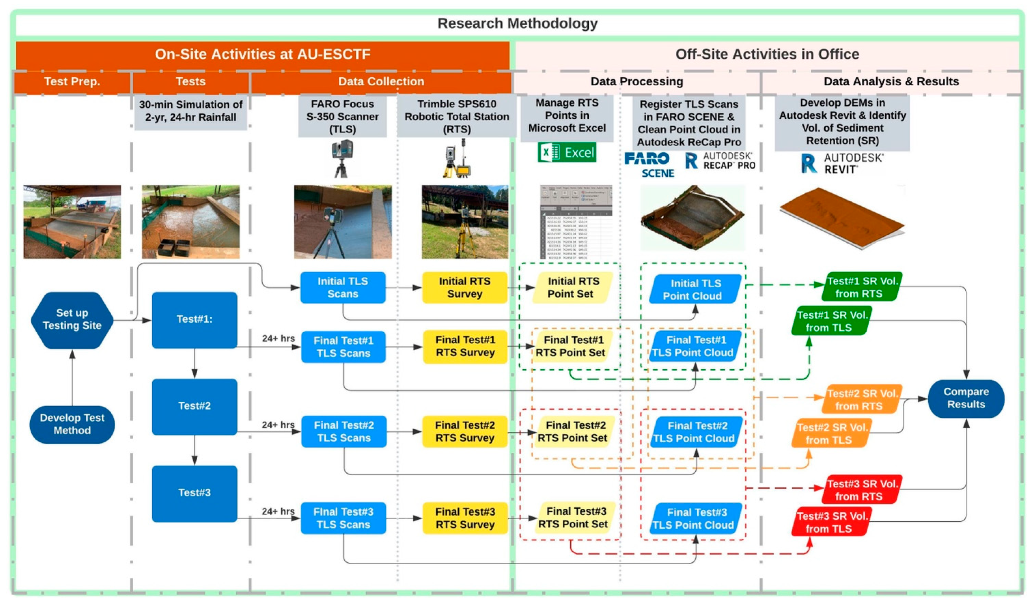
3. Materials and Methods
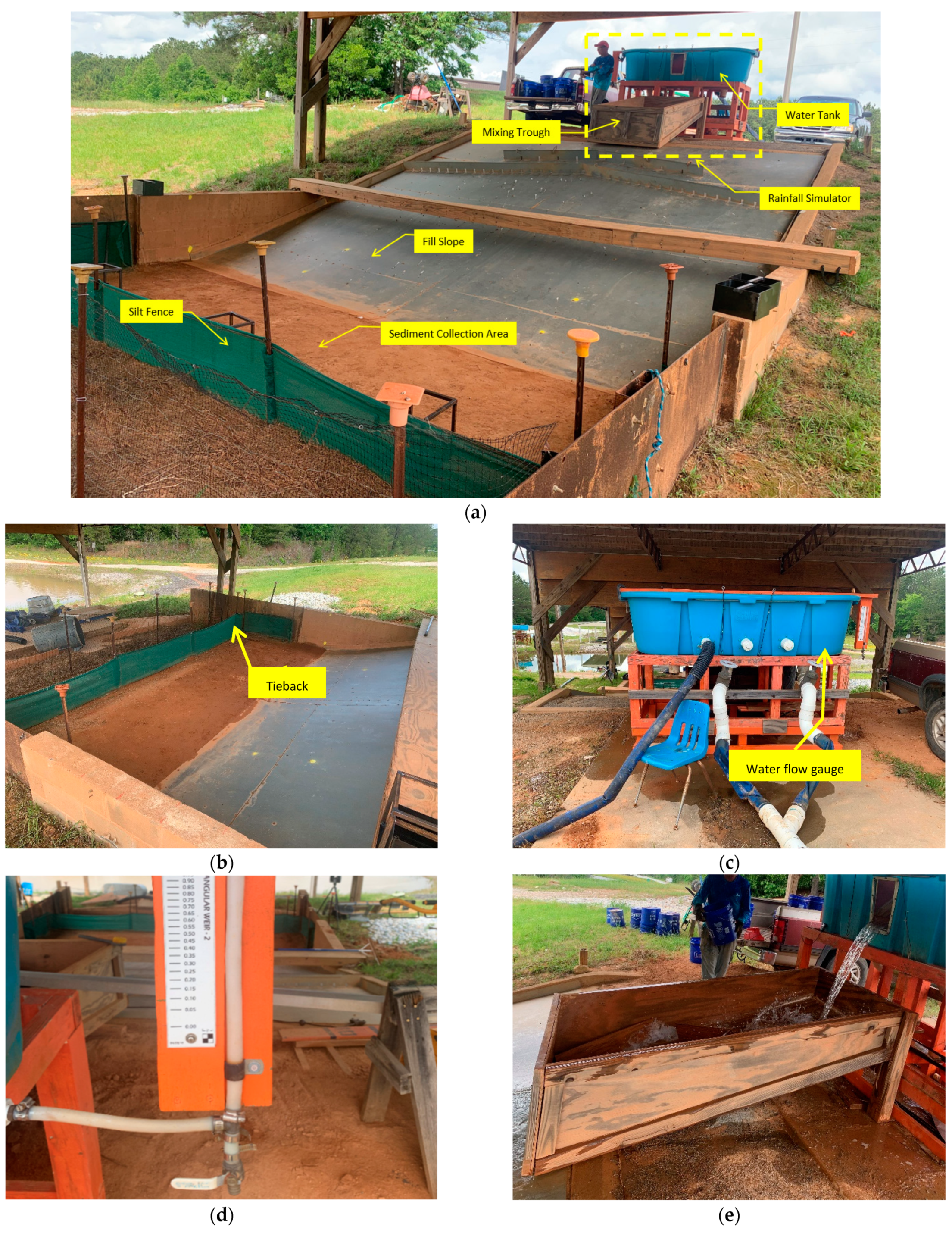
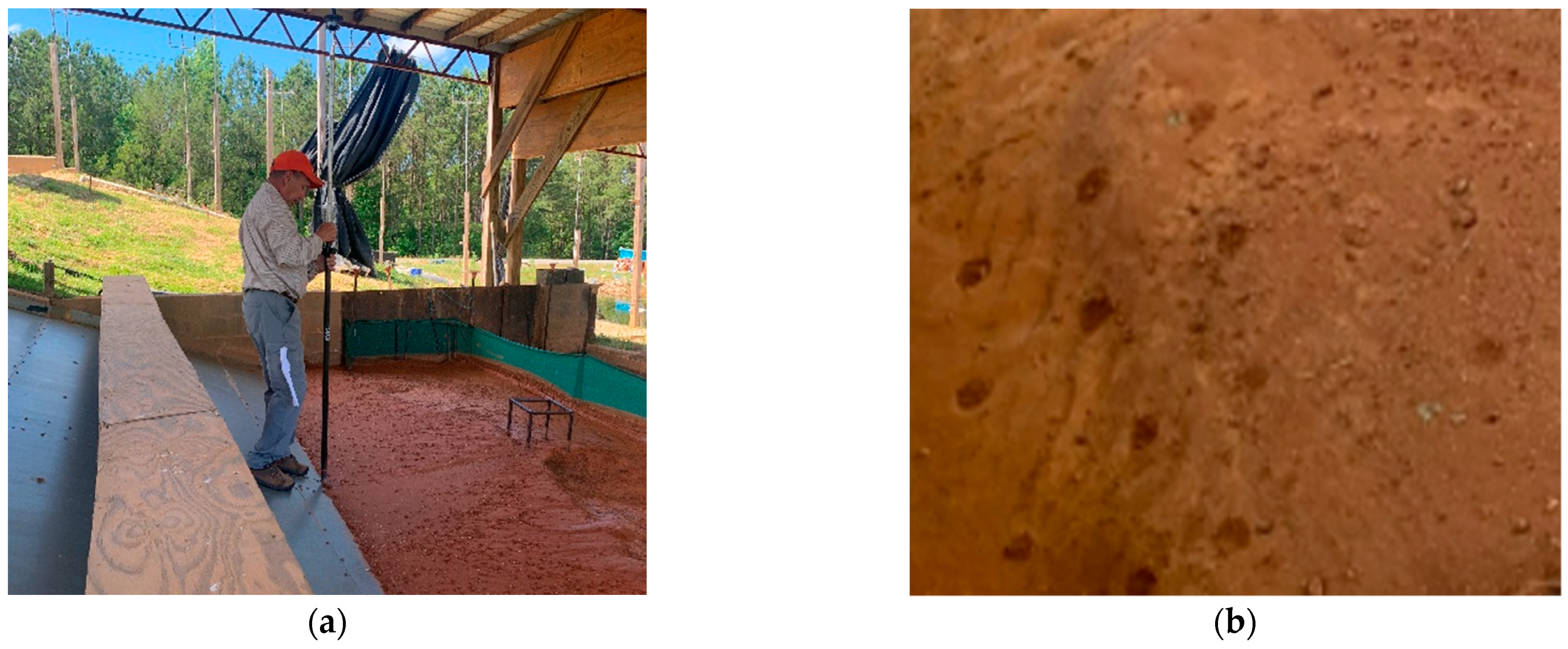
3.1. Experimental Apparatus and Equipment
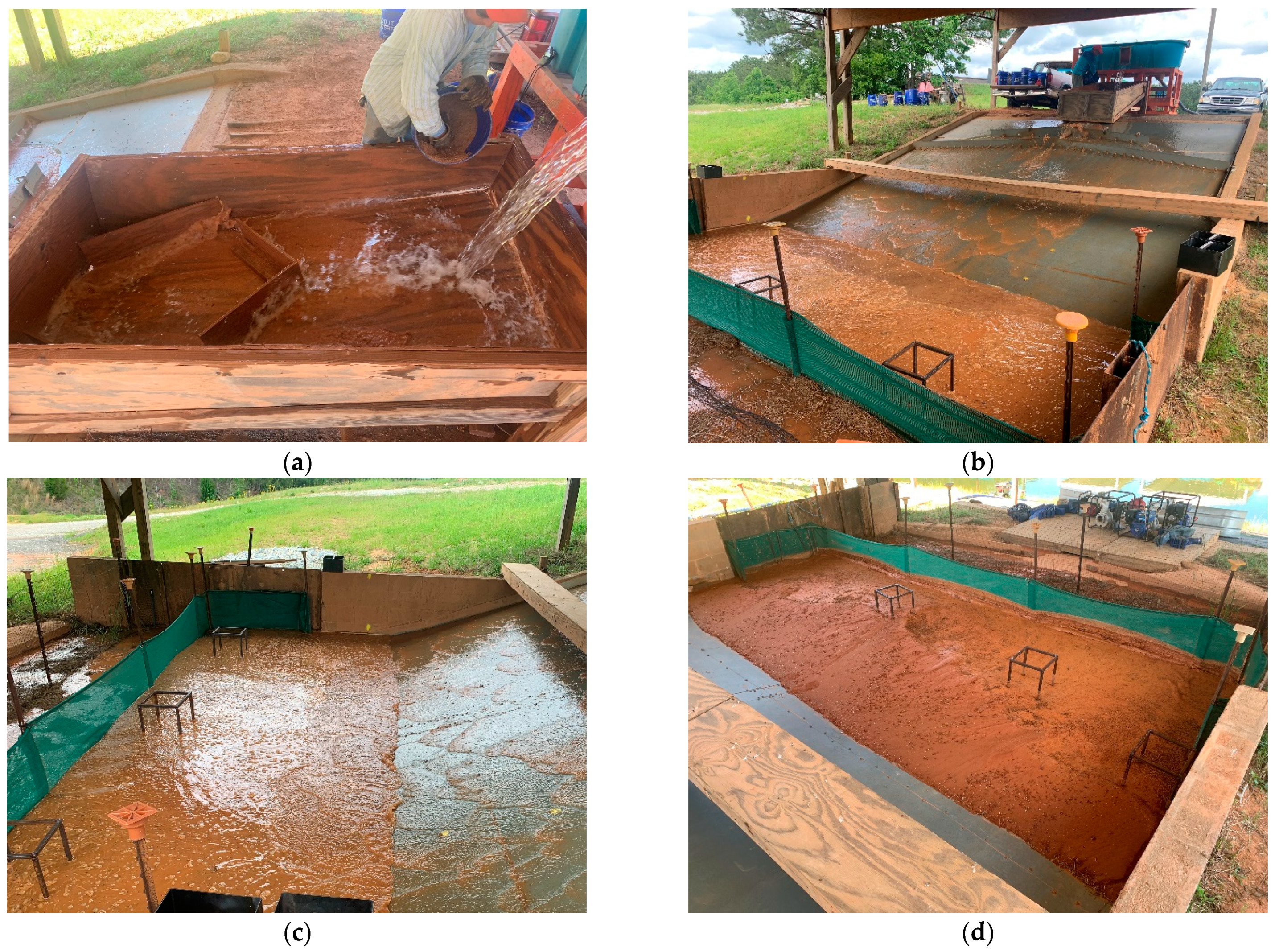
3.2. Experimental Procedure
3.3. Data Collection
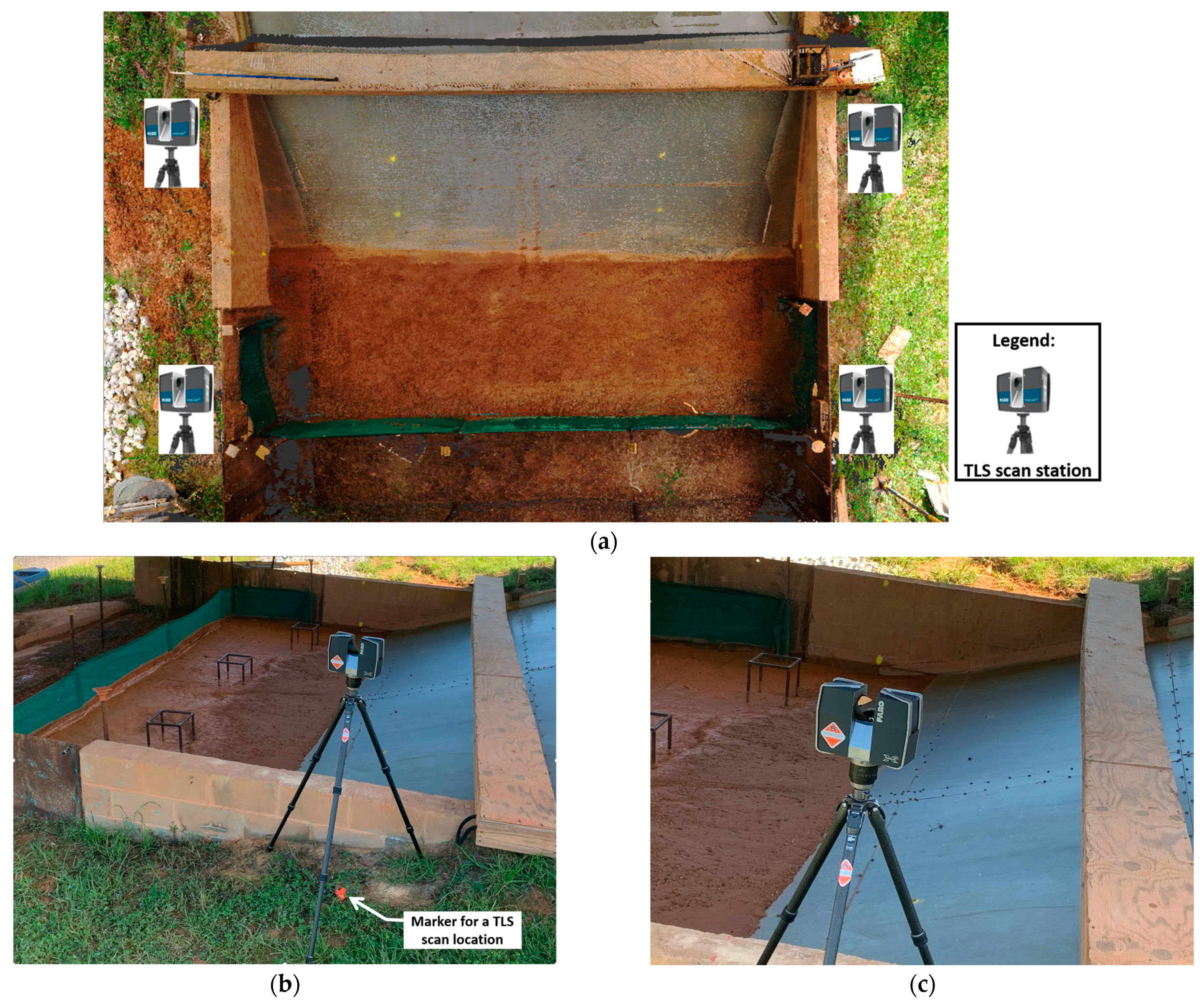
3.3.1. TLS Scanning
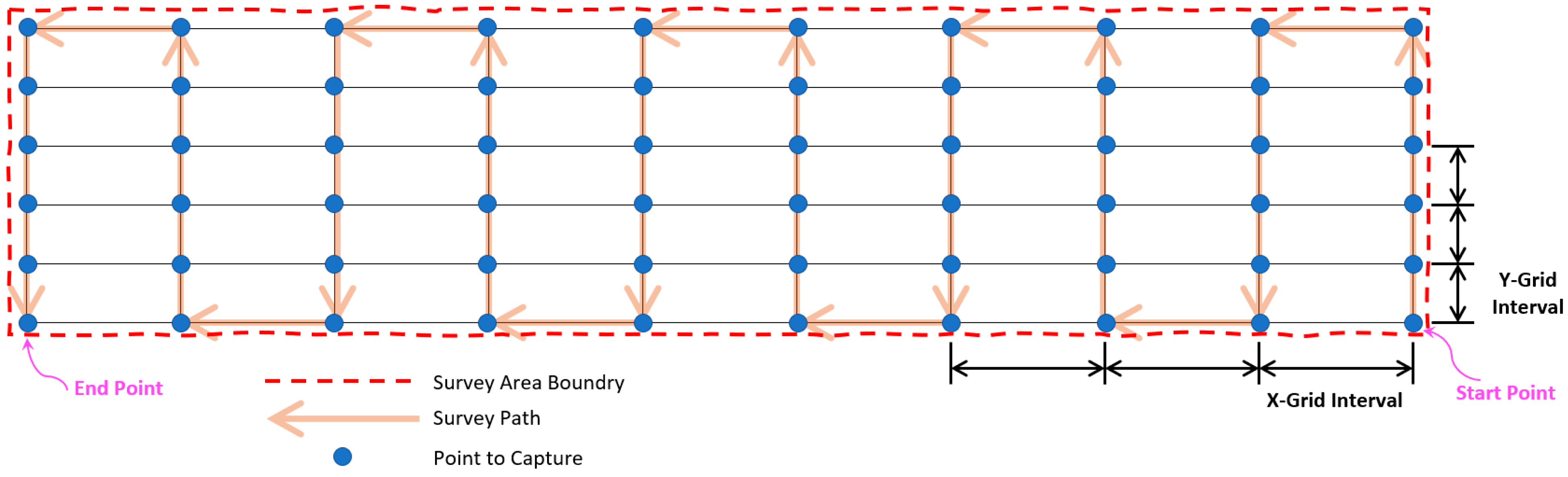
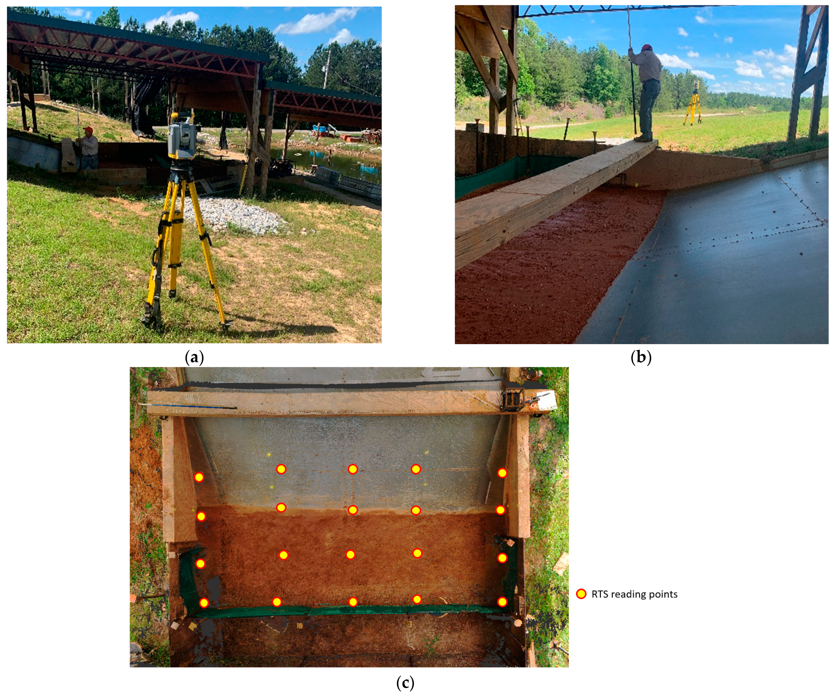
3.3.2. RTS Survey
4. Results and Discussion
4.1. Data Processing
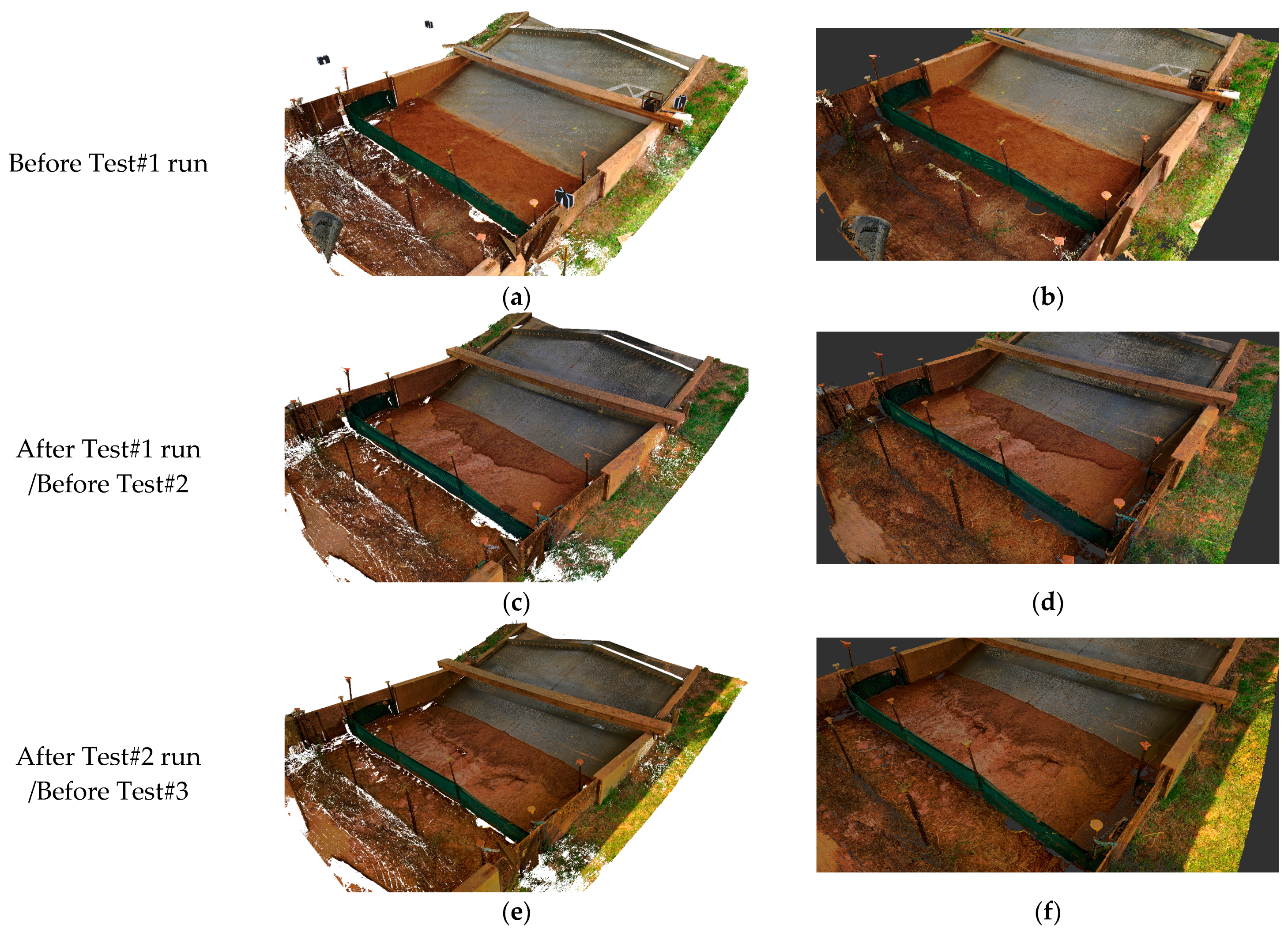
4.1.1. TLS Scans
4.1.2. RTS Points
4.2. Results
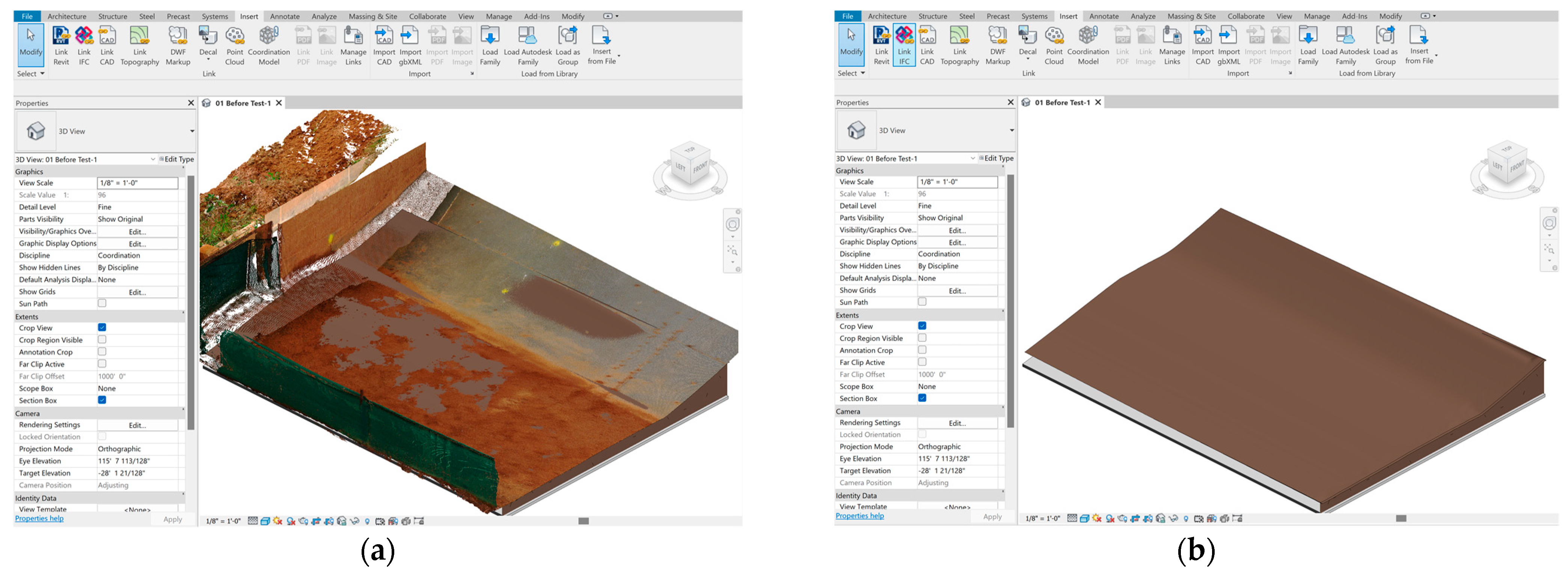
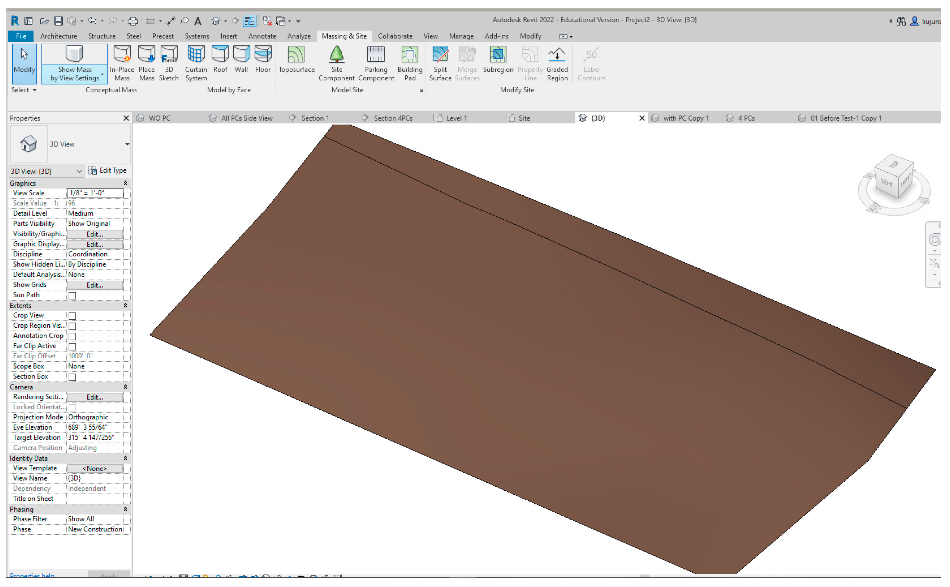
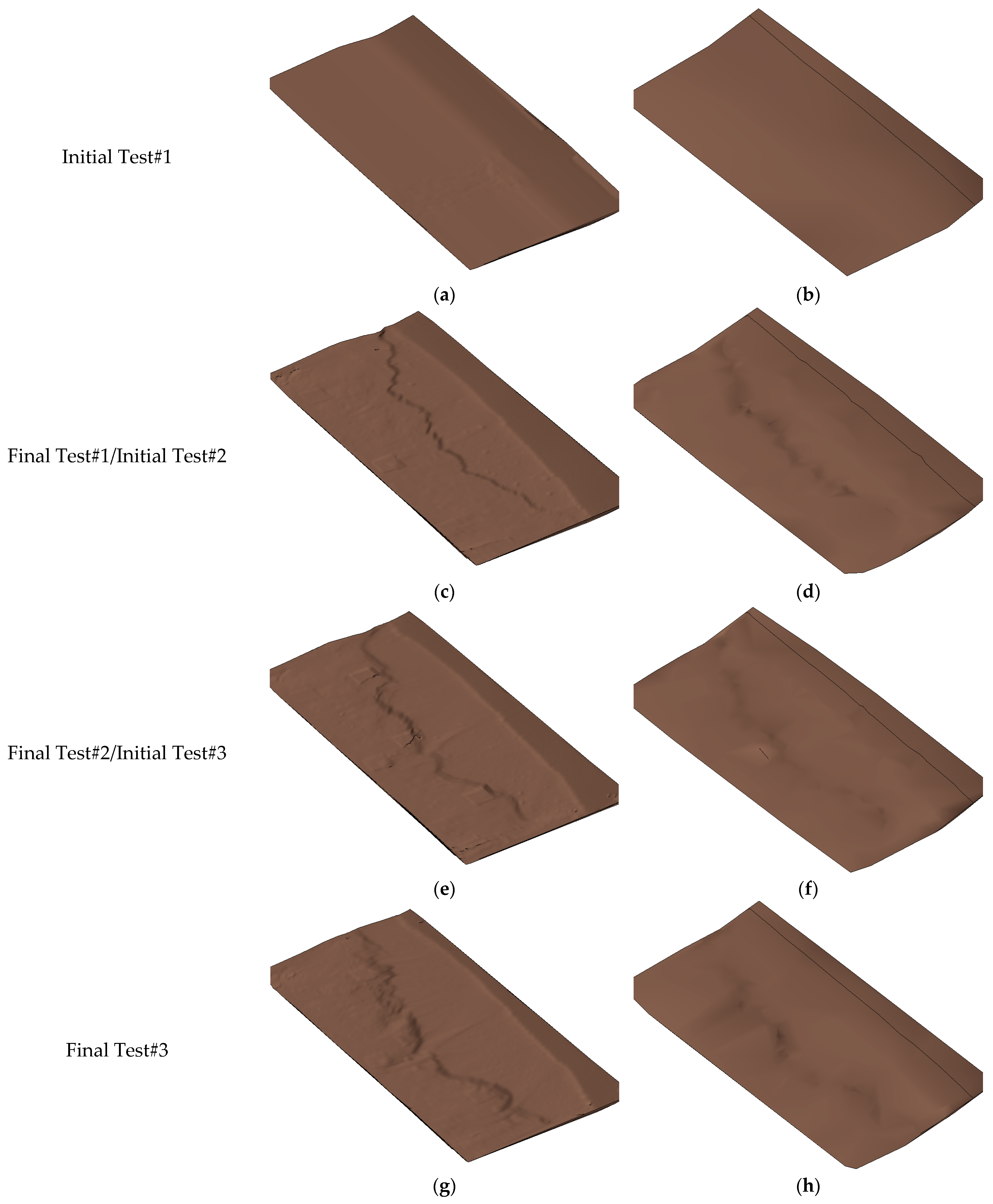
4.2.1. Developing DEMs in Revit
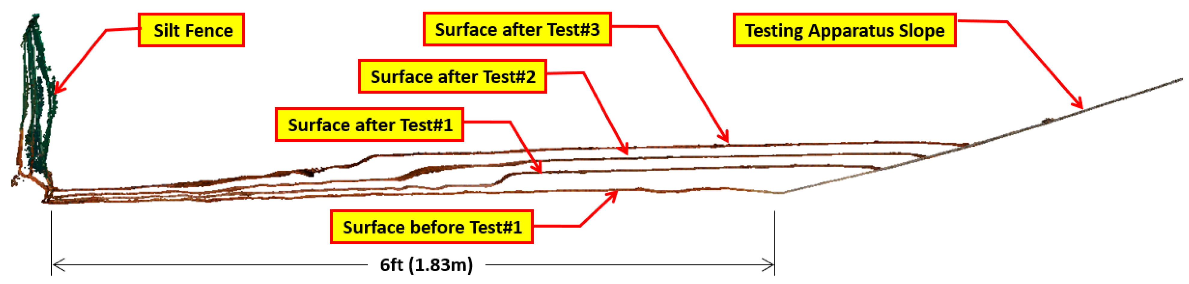
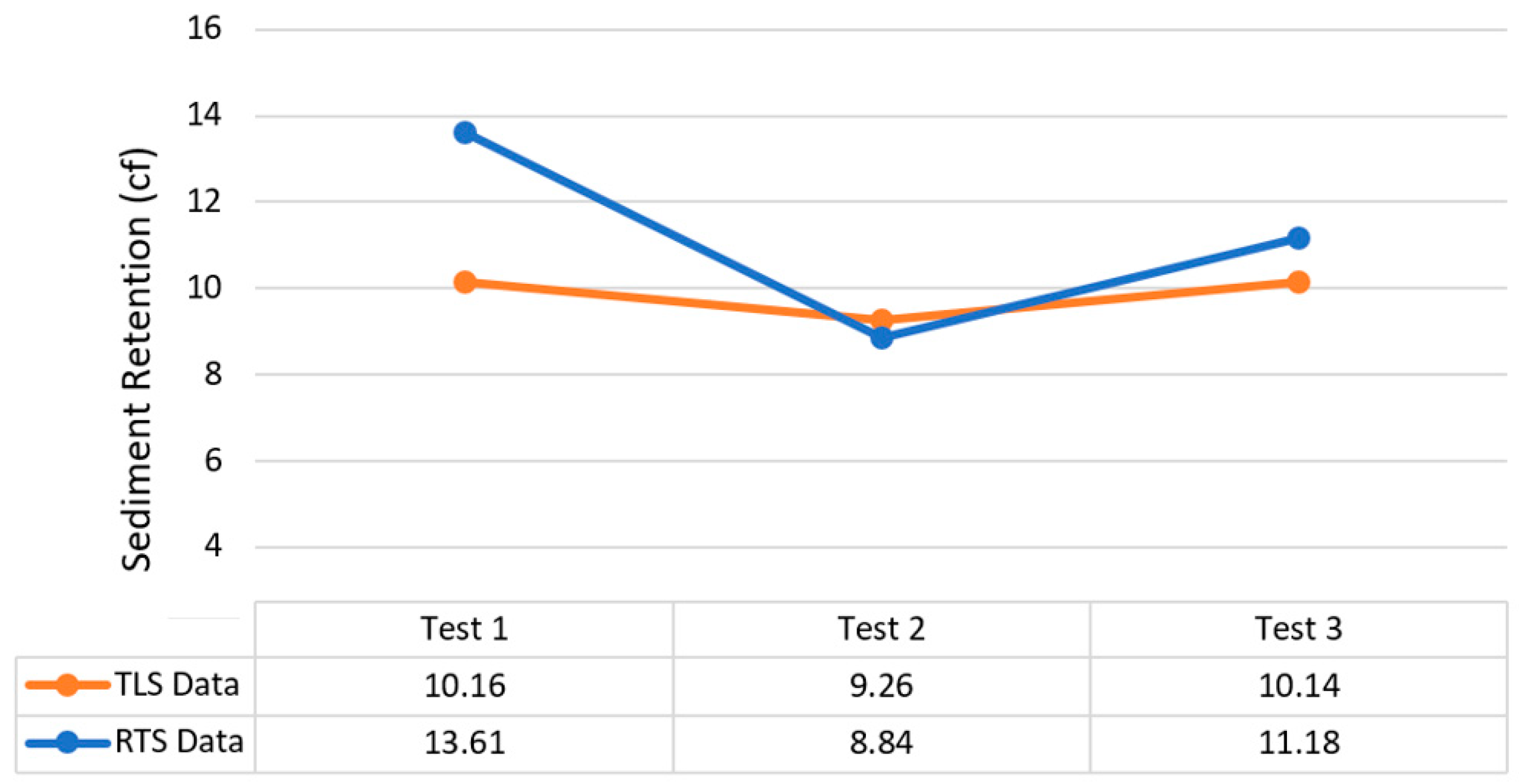
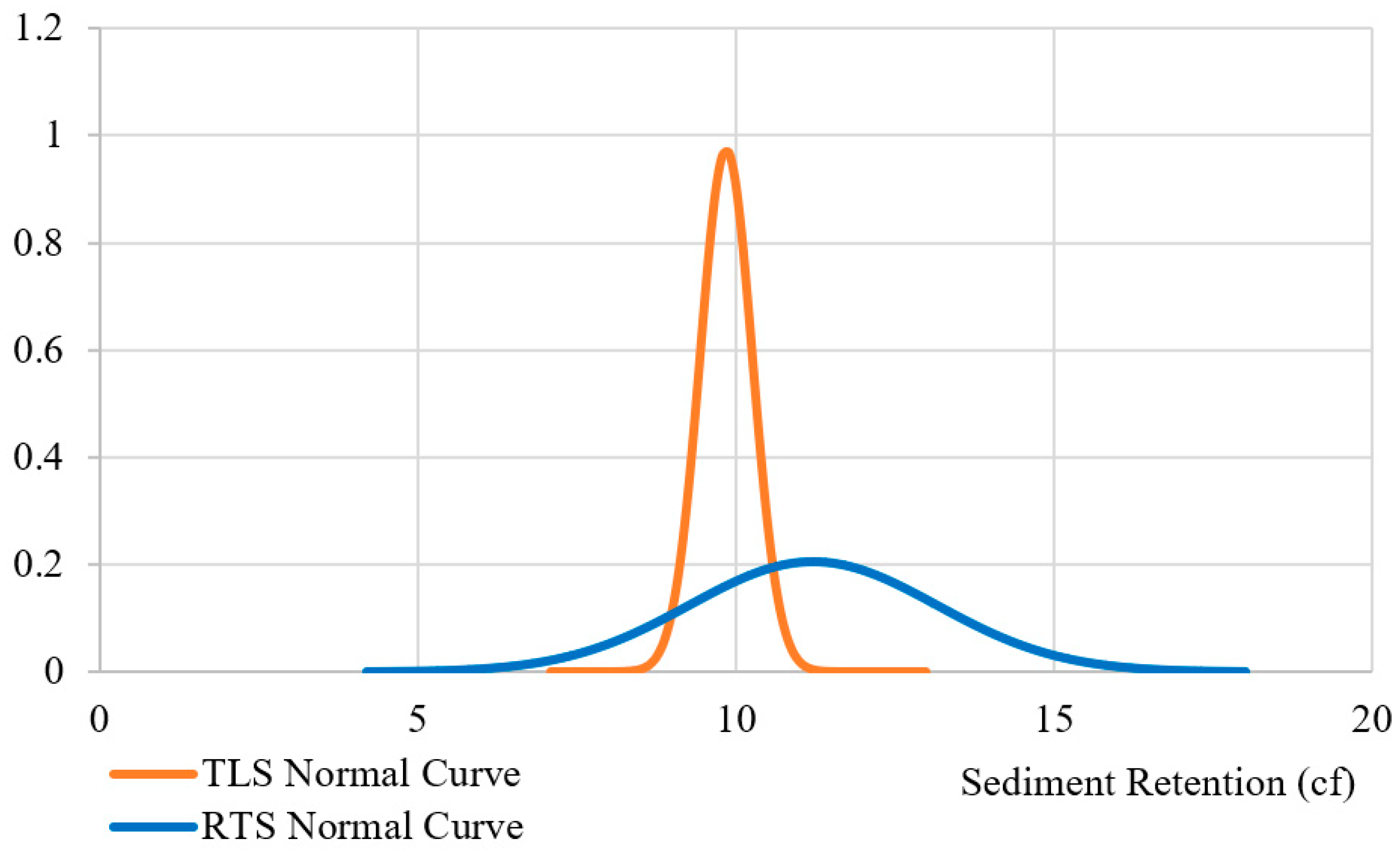
4.2.2. Using DEMs to Quantify Sediment Retention
4.3. Discussion
5. Conclusions and Recommendations for Future Research
Author Contributions
Funding
Institutional Review Board Statement
Informed Consent Statement
Data Availability Statement
Conflicts of Interest
References
- Toy, T.J.; Foster, G.R.; Renard, K.G. Soil Erosion: Processes, Prediction, Measurement, and Control; John Wiley & Sons: Hoboken, NJ, USA, 2002; ISBN 978-0-471-38369-7. [Google Scholar]
- Bugg, R.A.; Donald, W.; Zech, W.; Perez, M. Performance Evaluations of Three Silt Fence Practices Using a Full-Scale Testing Apparatus. Water 2017, 9, 502. [Google Scholar] [CrossRef]
- Whitman, J.B.; Zech, W.C.; Donald, W.N. Full-Scale Performance Evaluations of Innovative and Manufactured Sediment Barrier Practices. Transp. Res. Rec. J. Transp. Res. Board 2019, 2673, 284–297. [Google Scholar] [CrossRef]
- Barrett, M.E.; Malina, J.F.; Charbeneau, R.J. An Evaluation of Geotextiles for Temporary Sediment Control. Water Environ. Res. 1998, 70, 283–290. [Google Scholar] [CrossRef]
- Whitman, J.B.; Zech, W.C.; Donald, W.N.; LaMondia, J.J. Full-Scale Performance Evaluations of Various Wire-Backed Nonwoven Silt Fence Installation Configurations. Transp. Res. Rec. 2018, 2672, 68–78. [Google Scholar] [CrossRef]
- Rhea, D. Roadside Guide to Clean Water: Sediment Barriers. Available online: https://extension.psu.edu/roadside-guide-to-clean-water-sediment-barriers (accessed on 15 December 2022).
- Whitman, J.B.; Zech, W.C.; Donald, W.N. Improvements in Small-Scale Standardized Testing of Geotextiles Used in Silt Fence Applications. Geotext. Geomembr. 2019, 47, 598–609. [Google Scholar] [CrossRef]
- Perez, M.A.; Zech, W.C.; Donald, W.N.; Turochy, R.; Fagan, B.G. Transferring Innovative Erosion and Sediment Control Research Results into Industry Practice. Water 2019, 11, 2549. [Google Scholar] [CrossRef]
- Yakar, M. Digital Elevation Model Generation by Robotic Total Station Instrument. Exp. Technol. 2009, 33, 52–59. [Google Scholar] [CrossRef]
- Landphair, H.; McFalls, J.; Peterson, B.; Li, M. Alternatives to Silt Fence for Temporary Sediment Control at Highway Construction Sites: Guidelines for TxDOT. 1997. Available online: https://www.semanticscholar.org/paper/Alternatives-to-Silt-Fence-for-Temporary-Sediment-Landphair-McFalls/d98246d48bfc6ad652d691099926929abd5cf060 (accessed on 15 December 2022).
- DeMoranville, C.; Sandler, H. Erosion & Sediment Control BMP: Publications UMass Cranberry Station. Available online: https://www.umass.edu/cranberry/pubs/bmp_erosion.html (accessed on 15 December 2022).
- Whitman, J.B.; Perez, M.A.; Zech, W.C.; Donald, W.N. Practical Silt Fence Design Enhancements for Effective Dewatering and Stability. J. Irrig. Drain. Eng. 2021, 147, 04020039. [Google Scholar] [CrossRef]
- Gogo-Abite, I.; Chopra, M. Performance Evaluation of Two Silt Fence Geotextiles Using a Tilting Test-Bed with Simulated Rainfall. Geotext. Geomembr. 2013, 39, 30–38. [Google Scholar] [CrossRef]
- Keener, H.M.; Faucette, B.; Klingman, M.H. Flow-through Rates and Evaluation of Solids Separation of Compost Filter Socks versus Silt Fence in Sediment Control Applications. J. Environ. Qual. 2007, 36, 742–752. [Google Scholar] [CrossRef]
- Zech, W.C.; Halverson, J.L.; Clement, T.P. Intermediate-Scale Experiments to Evaluate Silt Fence Designs to Control Sediment Discharge from Highway Construction Sites. J. Hydrol. Eng. 2008, 13, 497–504. [Google Scholar] [CrossRef]
- Zimmie, T.F.; Kamalzare, M. Measuring the Rate of Sediment Transport and Erosion in Physical Model Testing. In Proceedings of the Innovations in Geotechnical Engineering, Orlando, FL, USA, 5–10 March 2018; American Society of Civil Engineers: Orlando, FL, USA, 2018; pp. 330–341. [Google Scholar]
- Tran, T.V.; Tucker-Kulesza, S.E.; Bernhardt, M. Soil Surface Roughness and Turbidity Measurements in Erosion Testing. IFCEE 2018, 2018, 506–515. [Google Scholar] [CrossRef]
- Keim, R.F.; Skaugset, A.E.; Bateman, D.S. Digital Terrain Modeling of Small Stream Channels with a Total-Station Theodolite. Adv. Water Resour. 1999, 23, 41–48. [Google Scholar] [CrossRef]
- Eltner, A.; Baumgart, P. Accuracy Constraints of Terrestrial Lidar Data for Soil Erosion Measurement: Application to a Mediterranean Field Plot. Geomorphology 2015, 245, 243–254. [Google Scholar] [CrossRef]
- Luffman, I.; Nandi, A.; Luffman, B. Comparison of Geometric and Volumetric Methods to a 3D Solid Model for Measurement of Gully Erosion and Sediment Yield. Geosciences 2018, 8, 86. [Google Scholar] [CrossRef]
- Li, L.; Lan, H.; Peng, J. Loess Erosion Patterns on a Cut-Slope Revealed by LiDAR Scanning. Eng. Geol. 2020, 268, 105516. [Google Scholar] [CrossRef]
- Resop, J.P.; Hession, W.C. Terrestrial Laser Scanning for Monitoring Streambank Retreat: Comparison with Traditional Surveying Techniques. J. Hydraul. Eng. 2010, 136, 794–798. [Google Scholar] [CrossRef]
- Myers, D.T.; Rediske, R.R.; McNair, J.N. Measuring Streambank Erosion: A Comparison of Erosion Pins, Total Station, and Terrestrial Laser Scanner. Water 2019, 11, 1846. [Google Scholar] [CrossRef]
- Danino, D.; Svoray, T.; Thompson, S.; Cohen, A.; Crompton, O.; Volk, E.; Argaman, E.; Levi, A.; Cohen, Y.; Narkis, K.; et al. Quantifying Shallow Overland Flow Patterns Under Laboratory Simulations Using Thermal and LiDAR Imagery. Water Resour. Res. 2021, 57, e2020WR028857. [Google Scholar] [CrossRef]
- Victoriano, A.; Brasington, J.; Guinau, M.; Furdada, G.; Cabré, M.; Moysset, M. Geomorphic Impact and Assessment of Flexible Barriers Using Multi-Temporal LiDAR Data: The Portainé Mountain Catchment (Pyrenees). Eng. Geol. 2018, 237, 168–180. [Google Scholar] [CrossRef]
- Heritage, G.; Hetherington, D. Towards a Protocol for Laser Scanning in Fluvial Geomorphology. Earth Surf. Process Landf. 2007, 32, 66–74. [Google Scholar] [CrossRef]
- Li, H. Investigation of Highway Stormwater Management Pond Capacity for Flood Detention and Water Quality Treatment Retention via Remote Sensing Data and Conventional Topographic Survey. Transp. Res. Rec. 2020, 2674, 514–527. [Google Scholar] [CrossRef]
- Valentini, E.; Taramelli, A.; Cappucci, S.; Filipponi, F.; Nguyen Xuan, A. Exploring the Dunes: The Correlations between Vegetation Cover Pattern and Morphology for Sediment Retention Assessment Using Airborne Multisensor Acquisition. Remote Sens. 2020, 12, 1229. [Google Scholar] [CrossRef]
- James, L.A.; Watson, D.G.; Hansen, W.F. Using LiDAR Data to Map Gullies and Headwater Streams under Forest Canopy: South Carolina, USA. CATENA 2007, 71, 132–144. [Google Scholar] [CrossRef]
- Li, L.; Nearing, M.A.; Nichols, M.H.; Polyakov, V.O.; Cavanaugh, M.L. Using Terrestrial LiDAR to Measure Water Erosion on Stony Plots under Simulated Rainfall. Earth Surf. Process Landf. 2020, 45, 484–495. [Google Scholar] [CrossRef]
- Bailey, G. Challenges in Approaching the Detection Limits for Hillslope Erosion Using Terrestrial Laser Scanning. Master’s Thesis, University of Tennessee, Knoxville, TN, USA, 2022. [Google Scholar]
- Bugg, R.A.; Donald, W.N.; Zech, W.C.; Perez, M.A. Improvements in Standardized Testing for Evaluating Sediment Barrier Performance: Design of a Full-Scale Testing Apparatus. J. Irrig. Drain. Eng. 2017, 143, 04017029. [Google Scholar] [CrossRef]
- FARO Focus Laser Scanner|FARO. Available online: https://www.faro.com/en/Products/Hardware/Focus-Laser-Scanners (accessed on 19 December 2022).
- Trimble S5|Robotic Total Stations|Trimble Geospatial. Available online: https://geospatial.trimble.com/products-and-solutions/trimble-s5 (accessed on 16 December 2022).
- Crumal, Z. What Is a Robotic Total Station? Here’s Everything You Need to Know. Available online: https://bim360resources.autodesk.com/connect-construct/what-is-a-robotic-total-station-heres-everything-you-need-to-know (accessed on 17 December 2022).
- FARO® SCENE 3D Point Cloud Software|FARO. Available online: https://www.faro.com/en/Products/Software/SCENE-Software (accessed on 26 November 2022).
- ReCap Software|What Is ReCap Pro?|Autodesk. Available online: https://www.autodesk.com/products/recap/overview (accessed on 26 November 2022).
- Getting Started with As-Built for Autodesk Revit. Available online: https://knowledge.faro.com/Software/As-Built/As-Built_for_Autodesk_Revit/Getting_Started_with_As-Built_for_Autodesk_Revit (accessed on 22 December 2022).
- Palcak, M.; Kudela, P.; Fandakova, M.; Kordek, J. Utilization of 3D Digital Technologies in the Documentation of Cultural Heritage: A Case Study of the Kunerad Mansion (Slovakia). Appl. Sci. 2022, 12, 4376. [Google Scholar] [CrossRef]


| TLS Scan Set | Mean Point Error | Max. Point Error | Min. Overlap |
|---|---|---|---|
| Before Test#1 run | 0.9 mm | 1.2 mm | 71.1% |
| After Test#1 run | 0.8 mm | 1.0 mm | 73.2% |
| After Test#2 run | 0.7 mm | 0.9 mm | 74.1% |
| After Test#3 run | 0.8 mm | 1.0 mm | 73.3% |
| RTS Capture Stage | Number of Points | Scatter Chart of Captured Points |
|---|---|---|
| Before Test#1 run | 20 |  |
| After Test#1 run | 271 |  |
| After Test#2 run | 243 | 2.55 |
| After Test#3 run | 178 |  |
| SR Vol. Calculated from TLS DEMs | SR Vol. Calculated from RTS DEMs | |||||
|---|---|---|---|---|---|---|
| Net Cut/Fill | Fill | Cut | Net Cut/Fill | Fill | Cut | |
| Test#1 | 10.16 cf (0.288 m3) | 10.60 cf (0.300 m3) | 0.44 cf (0.012 m3) | 13.61 cf (0.386 m3) | 13.91 cf (0.394 m3) | 0.30 cf (0.008 m3) |
| Test#2 | 9.26 cf (0.262 m3) | 9.32 cf (0.264 m3) | 0.06 cf (0.002 m3) | 8.84 cf (0.250 m3) | 9.48 cf (0.268 m3) | 0.64 cf (0.018 m3) |
| Test#3 | 10.14 cf (0.287 m3) | 10.18 cf (0.288 m3) | 0.04 cf (0.001 m3) | 11.18 cf (0.317 m3) | 11.75 cf (0.333 m3) | 0.57 cf (0.016 m3) |
Disclaimer/Publisher’s Note: The statements, opinions and data contained in all publications are solely those of the individual author(s) and contributor(s) and not of MDPI and/or the editor(s). MDPI and/or the editor(s) disclaim responsibility for any injury to people or property resulting from any ideas, methods, instructions or products referred to in the content. |
© 2023 by the authors. Licensee MDPI, Basel, Switzerland. This article is an open access article distributed under the terms and conditions of the Creative Commons Attribution (CC BY) license (https://creativecommons.org/licenses/by/4.0/).
Share and Cite
Liu, J.; Bugg, R.A.; Fisher, C.W. Advancing Erosion Control Analysis: A Comparative Study of Terrestrial Laser Scanning (TLS) and Robotic Total Station Techniques for Sediment Barrier Retention Measurement. Geomatics 2023, 3, 345-363. https://doi.org/10.3390/geomatics3020019
Liu J, Bugg RA, Fisher CW. Advancing Erosion Control Analysis: A Comparative Study of Terrestrial Laser Scanning (TLS) and Robotic Total Station Techniques for Sediment Barrier Retention Measurement. Geomatics. 2023; 3(2):345-363. https://doi.org/10.3390/geomatics3020019
Chicago/Turabian StyleLiu, Junshan, Robert A. Bugg, and Cort W. Fisher. 2023. "Advancing Erosion Control Analysis: A Comparative Study of Terrestrial Laser Scanning (TLS) and Robotic Total Station Techniques for Sediment Barrier Retention Measurement" Geomatics 3, no. 2: 345-363. https://doi.org/10.3390/geomatics3020019