
Remote Sensing Image Scene Classification: Advances and Open Challenges


Abstract
:1. Introduction
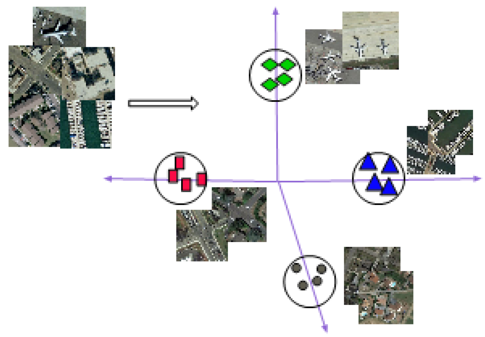
- Complex spatial arrangements. Remotely sensed images have significant variations in the semantics (for instance, the scene images; of agriculture, airport, commercial areas, and residential areas are typical examples of varying scene image semantics). Extracting the semantic features from images requires effective computer vision techniques.
- Low inter-class variance. Some scene images are similar (e.g., agriculture and forest, dense residential areas, and residential-area). This characteristic is referred to as low intra-class variance. Achieving accurate scene classification under this circumstance requires well-calibrated computer vision techniques.
- High intra-class variance. Those same class scene images are commonly taken at varying angles, scales, and viewpoints. This diverse variation of same-class images requires well-designed computer vision approaches that can extract the same pattern features from the remotely sensed images regardless of their variations.
- Noise: Remotely sensed images are taken under varying atmospheric conditions and at different seasons. The scene images may have variable illumination conditions and require robust feature-learning techniques against varying weather circumstances.
- This survey presents image-feature analysis methods, strengths, and shortcomings.
- This paper discusses the CNN architectures commonly adopted for the scene classification of remote sensing imagery.
- We present the deep learning models that integrate both knowledge and data architectures, which are transformer-based and ontology-based models.
- This paper discusses the advanced machine learning implementation frameworks; they are commonly utilized in implementing deep learning solutions in remote sensing image scene classification.
- We discuss the properties of remote sensing datasets and their uniqueness in evaluating the different feature learning approaches.
- This work presents the performance evaluation metrics upon which the feature analysis methods are evaluated to determine their scene classification effectiveness.
- This paper discusses the open opportunities that need to be addressed by the remote sensing community.
2. Image Feature Learning Approaches
2.1. Pixel-Based Feature Learning Methods
2.1.1. Local Binary Patterns
2.1.2. Multi-Scale Completed Local Binary Pattern
2.1.3. Distinctive Features Scale-Invariant
- Scale-space extrema detection: a cascading algorithm identifies candidate points, which are further inspected. Once key candidate locations and scales were established that can be replicated with different views on the same object, the detection of locations follows that are invariant to scale changes of an image through looking for possible features across every probable scale. The Scale-space search algorithm accomplishes the task mentioned above.
- Localization of keypoint features: This is the process of establishing key candidate features by comparing neighbors to find a precise fit of the nearby data for location and scales of the primary curvatures. Points with low contrast (sensitive to noise) or unsatisfactorily localized along the edges are rejected.
- Orientation allocation: A consistent assignment is done for every keypoint depending on local image feature attributes in this step. The keypoint descriptor is formulated for orientation; therefore, they are invariant to image rotations. The keypoint descriptors then generate orientation histograms from gradient orientations based on sample points within a region surrounding the keypoint. A histogram contains 36 bins spanning 360 degrees of orientation. The gradient magnitudes determine every sample on the histogram, and a Gaussian-weighted circular window [31]. Dominant directions of local gradients are ’peaks’ of orientation histograms. The highest peak detected in the histogram and other local peaks above 80% of the highest peak apply to generate a key point on an orientation histogram.
- Local image descriptor: The operations described above, i.e., (detection of scale-space, keypoint localization, and orientation assignment) assigned to an image the (scale, orientation, and location) for each keypoint. These parameters create a repeatable local 2D coordinate system that characterizes the local region of an image, thereby providing an invariant feature descriptor [31]
2.2. Mid-Level Feature Learning Methods
2.2.1. The Bag of Visual Words
2.2.2. Fisher Vectors
2.3. High-Level Feature Learning Methods
2.3.1. Bag of Convolutional Features
2.3.2. Adaptive Deep Pyramid Matching
2.3.3. Deep Salient Feature-Based Anti-Noise Transfer Network (DSFBA-NTN)
2.3.4. Joint Learning Center Points and Deep Metrics
3. Deep Learning Architectures
3.1. Autoencoders and Stacked Autoencoders
3.2. AlexNet
3.3. VGGNet
- Its filters use receptive fields of size 3. These are smaller than AlexNet ( or ).
- On the same blocks, they contain the exact size of feature maps and the number of filters in every convolutional layer.
- The size of features increases in deeper layers; they double after every max-pool layer.
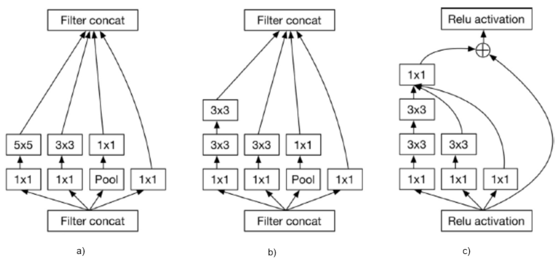
3.4. GoogleNet
Inception
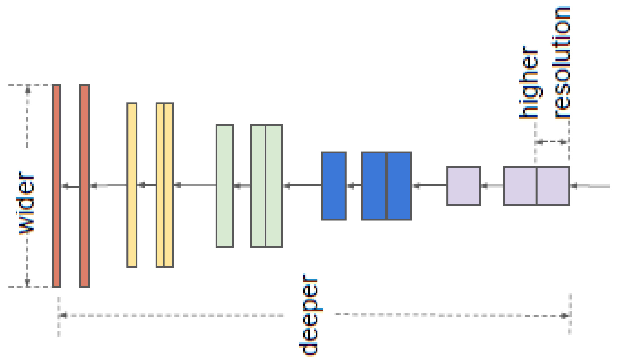
3.5. EfficientNet
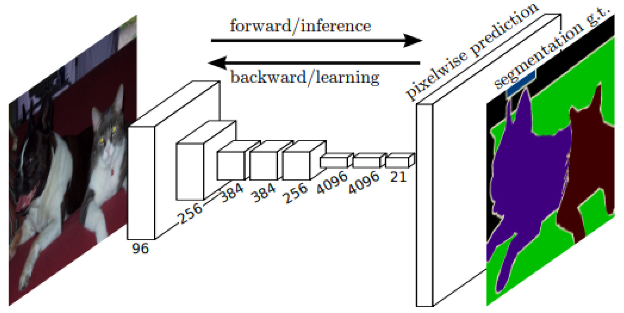
3.6. Fully Convolutional Networks
- Introduces skip connections to fuse information from different network depths to achieve multi-scale inferencing.
- Uses fully convolutional architecture model. This permits it to take arbitrary size images as inputs because in the absence of fully connected layers; no specific activation sizes are required at the end of the network.
- The FCN allows end-to-end learning through the encoder and decoder framework, which compresses and expands.
3.7. U-Net
3.8. Deep Residual
3.9. DeepResUnet
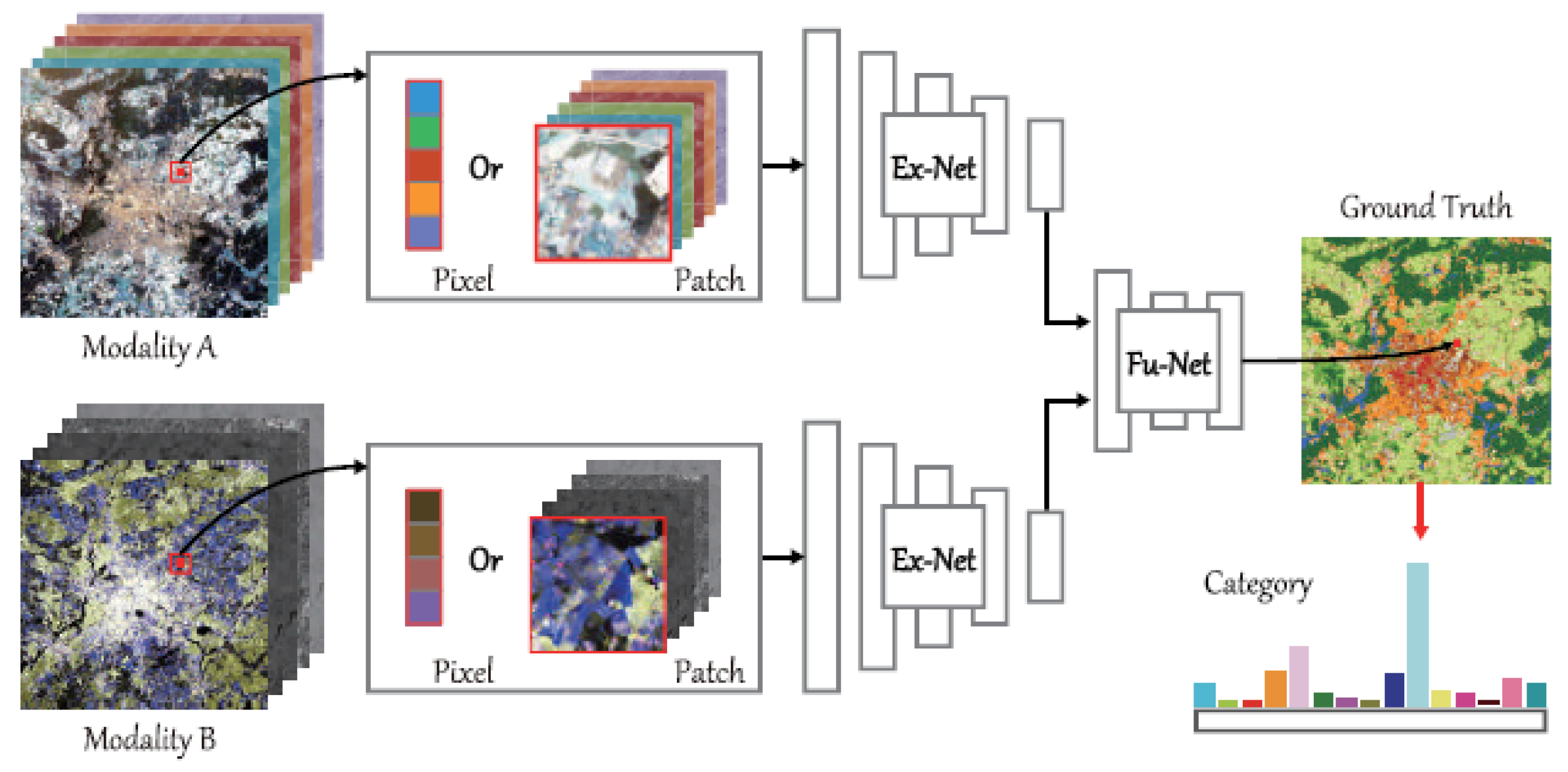
3.10. Unified Multimodal Data Analysis Deep Learning Architecture
4. Transformer-Based Deep Learning Models
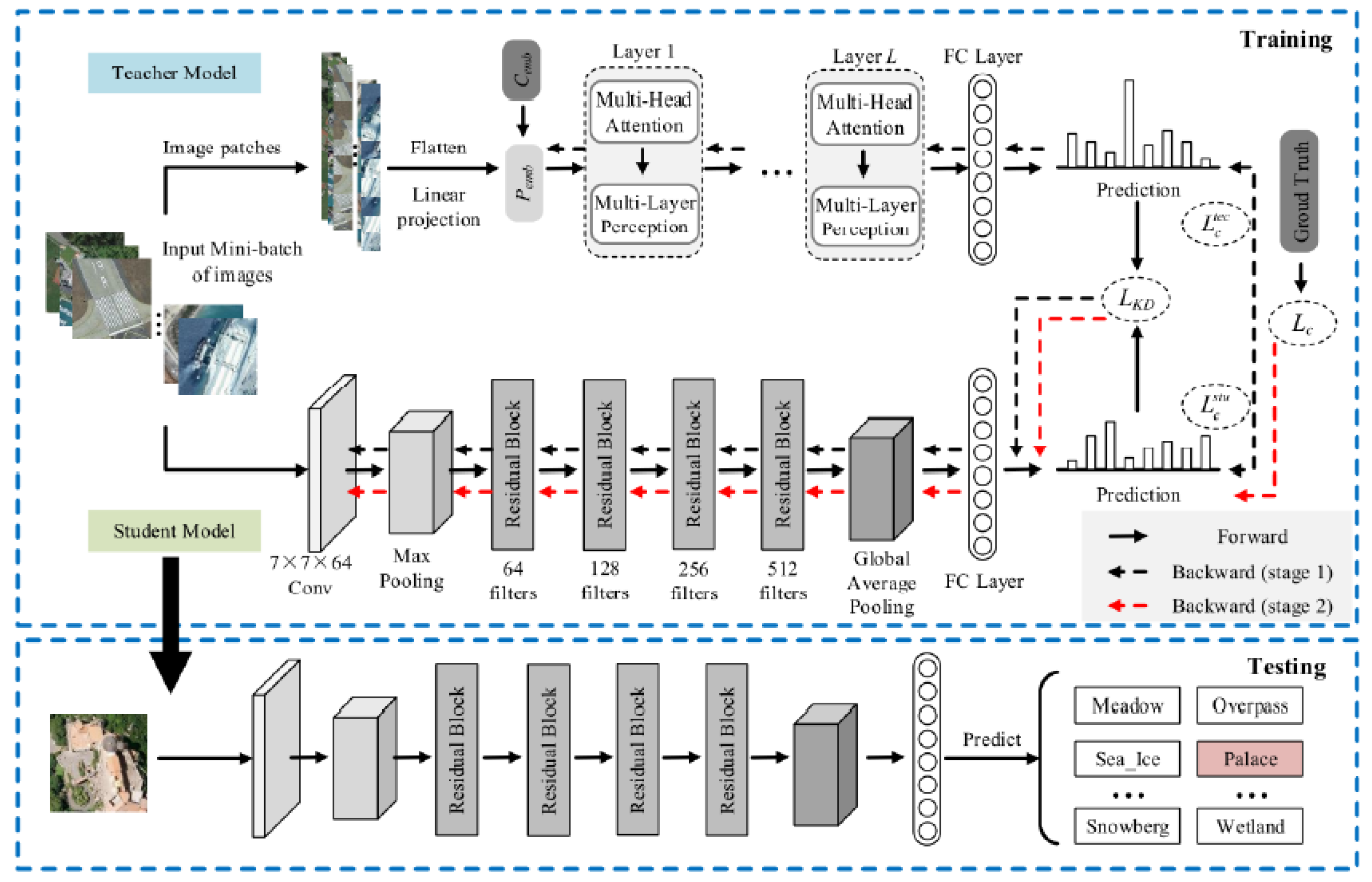
4.1. Excellent Teacher Network Guiding Small Networks (ET-GSNet)
4.2. Label-Free Self-Distillation Contrastive Learning with Transformer Architecture (LaST)
5. Machine Learning Algorithms
5.1. The Softmax Function
5.2. The Hinge-Loss Function
6. Deep Learning Open-Source Frameworks
6.1. TensorFlow
6.2. Caffe
6.3. Deeplearning4J
7. Remote Sensing Datasets for Models-Evaluation
7.1. UC Merced Dataset
7.2. WHURS Dataset
7.3. RSSCN7 Dataset
7.4. Aerial Image Dataset
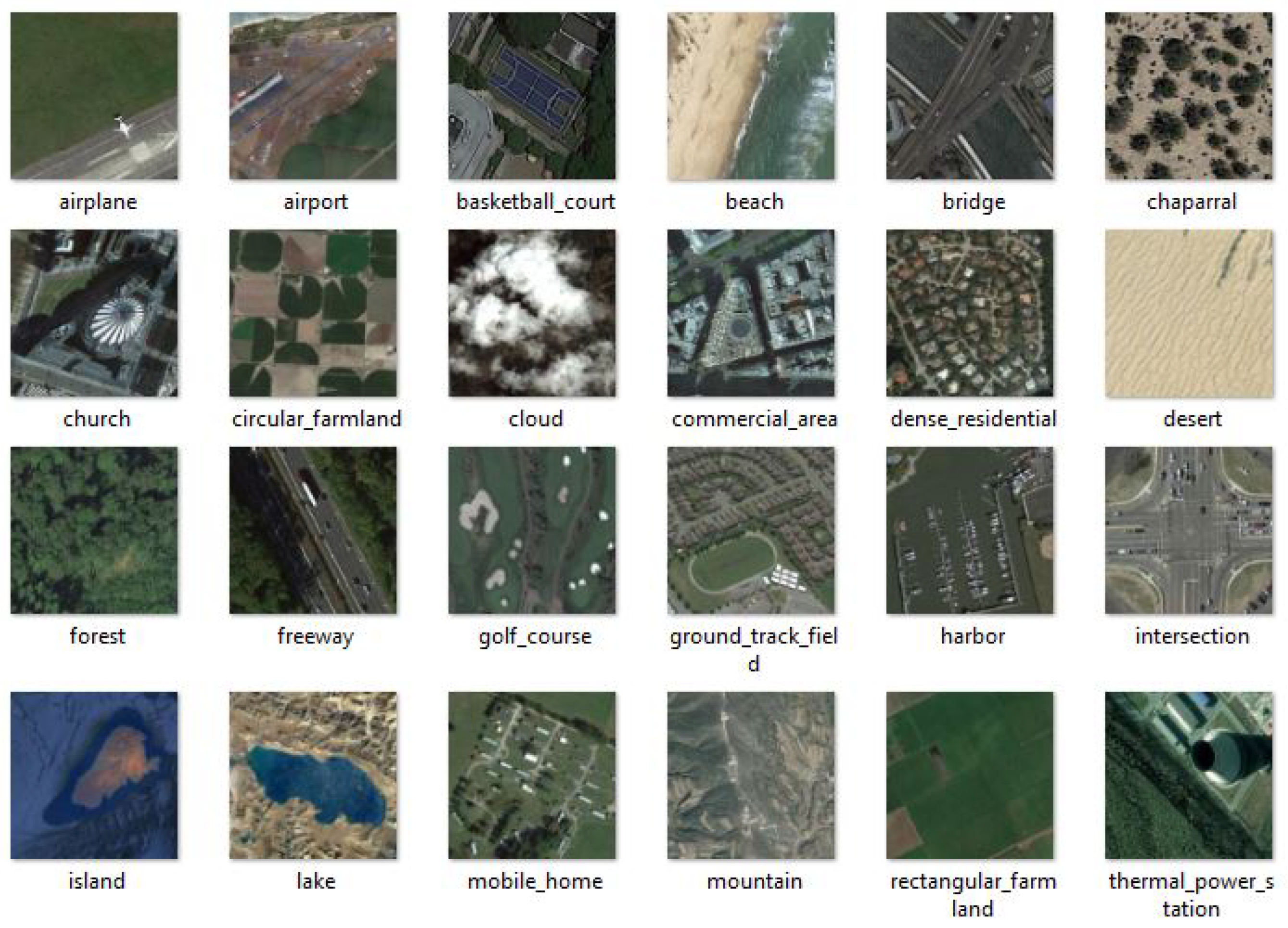
7.5. RESISC45 Dataset
7.6. Metrics Performance Evaluation
7.6.1. Overall Accuracy
7.6.2. Average Accuracy
7.6.3. Confusion Matrix
7.7. Scene Classification Performance Analysis of the State-of-the-Art
8. Discussions
9. Conclusions and Future Work
Author Contributions
Funding
Institutional Review Board Statement
Informed Consent Statement
Data Availability Statement
Conflicts of Interest
References
- Cheng, G.; Xie, X.; Han, J.; Guo, L.; Xia, G.-S. Remote Sensing Image Scene Classification Meets Deep Learning: Challenges, Methods, Benchmarks, and Opportunities. IEEE J. Sel. Top. Appl. Earth Obs. Remote Sens. 2020, 13, 3735–3756. [Google Scholar] [CrossRef]
- Cheng, G.; Han, J.; Lu, X. Remote Sensing Image Classification: Benchmark and State of the Art. Proc. IEEE 2017, 105, 1865–1883. [Google Scholar] [CrossRef]
- Xia, G.-S.; Hu, J.; Hu, F.; Shi, B.; Bai, X.; Zhong, Y.; Zhang, L.; Lu, X. AID: A Benchmark Data Set for Performance Evaluation of Aerial Scene Classification. IEEE Trans. Geosci. Remote Sens. 2017, 55, 3965–3981. [Google Scholar] [CrossRef]
- Zhou, Q.; Zheng, B.; Zhu, W.; Latecki, L.J. Multi-scale context for scene labeling via flexible segmentation graph. Pattern Recognit. 2016, 59, 312–324. [Google Scholar] [CrossRef]
- Zhou, B.; Khosla, A.; Lapedriza, A.; Oliva, A.; Torralba, A. Learning deep features for discriminative localization. In Proceedings of the IEEE Conference on Computer Vision and Pattern Recognition, Honolulu, HI, USA, 21–26 July 2016; pp. 2921–2929. [Google Scholar]
- He, K.; Zhang, X.; Ren, S.; Sun, J. Deep residual learning for image recognition. In Proceedings of the IEEE Conference on Computer Vision and Pattern Recognition, Honolulu, HI, USA, 21–26 July 2016; pp. 770–778. [Google Scholar]
- Bu, S.; Han, P.; Liu, Z.; Han, J. Scene parsing using inference embedded deep networks. Pattern Recognit. 2016, 59, 188–198. [Google Scholar] [CrossRef]
- Pohlen, T.; Hermans, A.; Mathias, M.; Leibe, B. Full-resolution residual networks for semantic segmentation in street scenes. In Proceedings of the IEEE Conference on Computer Vision and Pattern Recognition, Honolulu, HI, USA, 21–26 July 2017; pp. 4151–4160. [Google Scholar]
- Tombe, R.; Viriri, S. Adaptive Deep Co-Occurrence Feature Learning Based on Classifier-Fusion for Remote Sensing Scene Classification. IEEE J. Sel. Top. Appl. Earth Obs. Remote. Sens. 2020, 14, 155–164. [Google Scholar] [CrossRef]
- Boualleg, Y.; Farah, M.; Farah, I.R. Remote Sensing Scene Classification Using Convolutional Features and Deep Forest Classifier. IEEE Geosci. Remote Sens. Lett. 2019, 16, 1944–1948. [Google Scholar] [CrossRef]
- LeCun, Y.; Bengio, Y.; Hinton, G. Deep learning. Nature 2015, 521, 436–444. [Google Scholar] [CrossRef]
- Simonyan, K.; Zisserman, A. Very deep convolutional networks for large-scale image recognition. arXiv 2014, arXiv:1409.1556. [Google Scholar]
- Hu, F.; Xia, G.-S.; Hu, J.; Zhang, L. Transferring Deep Convolutional Neural Networks for the Scene Classification of High-Resolution Remote Sensing Imagery. Remote Sens. 2015, 7, 14680–14707. [Google Scholar] [CrossRef]
- Li, E.; Xia, J.; Du, P.; Lin, C.; Samat, A. Integrating Multilayer Features of Convolutional Neural Networks for Remote Sensing Scene Classification. IEEE Trans. Geosci. Remote Sens. 2017, 55, 5653–5665. [Google Scholar] [CrossRef]
- Yuan, B.; Han, L.; Gu, X.; Yan, H. Multi-deep features fusion for high-resolution remote sensing image scene classification. Neural Comput. Appl. 2020, 33, 2047–2063. [Google Scholar] [CrossRef]
- Liu, N.; Wan, L.; Zhang, Y.; Zhou, T.; Huo, H.; Fang, T. Exploiting Convolutional Neural Networks With Deeply Local Description for Remote Sensing Image Classification. IEEE Access 2018, 6, 11215–11228. [Google Scholar] [CrossRef]
- Xu, K.; Huang, H.; Deng, P.; Shi, G. Two-stream feature aggregation deep neural network for scene classification of remote sensing images. Inf. Sci. 2020, 539, 250–268. [Google Scholar] [CrossRef]
- Bazi, Y.; Al Rahhal, M.M.; Alhichri, H.; Alajlan, N. Simple Yet Effective Fine-Tuning of Deep CNNs Using an Auxiliary Classification Loss for Remote Sensing Scene Classification. Remote Sens. 2019, 11, 2908. [Google Scholar] [CrossRef]
- Krizhevsky, A.; Sutskever, I.; Hinton, G.E. Imagenet classification with deep convolutional neural networks. In Advances in Neural Information Processing Systems. Available online: https://papers.nips.cc/paper/2012/hash/c399862d3b9d6b76c8436e924a68c45b-Abstract.html (accessed on 30 December 2022).
- Ronneberger, O.; Fischer, P.; Brox, T. U-net: Convolutional networks for biomedical image segmentation. In International Conference on Medical Image Computing and Computer-Assisted Intervention; Springer: Berlin/Heidelberg, Germany, 2015; pp. 234–241. [Google Scholar]
- Jing, W.; Zhang, M.; Tian, D. Improved U-Net model for remote sensing image classification method based on distributed storage. J. Real-Time Image Process. 2020, 18, 1607–1619. [Google Scholar] [CrossRef]
- Badrinarayanan, V.; Kendall, A.; Cipolla, R. Segnet: A deep convolutional encoder-decoder architecture for image segmentation. IEEE Trans. Pattern Anal. Mach. Intell. 2017, 39, 2481–2495. [Google Scholar] [CrossRef]
- Yi, Y.; Zhang, Z.; Zhang, W.; Zhang, C.; Li, W.; Zhao, T. Semantic Segmentation of Urban Buildings from VHR Remote Sensing Imagery Using a Deep Convolutional Neural Network. Remote Sens. 2019, 11, 1774. [Google Scholar] [CrossRef]
- Xu, K.; Deng, P.; Huang, H. Vision Transformer: An Excellent Teacher for Guiding Small Networks in Remote Sensing Image Scene Classification. IEEE Trans. Geosci. Remote Sens. 2022, 60, 1–15. [Google Scholar] [CrossRef]
- Wang, X.; Zhu, J.; Yan, Z.; Zhang, Z.; Zhang, Y.; Chen, Y.; Li, H. LaST: Label-Free Self-Distillation Contrastive Learning With Transformer Architecture for Remote Sensing Image Scene Classification. IEEE Geosci. Remote Sens. Lett. 2022, 19, 1–5. [Google Scholar] [CrossRef]
- Deng, P.; Xu, K.; Huang, H. When CNNs Meet Vision Transformer: A Joint Framework for Remote Sensing Scene Classification. IEEE Geosci. Remote Sens. Lett. 2021, 19, 1–5. [Google Scholar] [CrossRef]
- Ge, Y.; Zhang, X.; Atkinson, P.M.; Stein, A.; Li, L. Geoscience-aware deep learning: A new paradigm for remote sensing. Sci. Remote Sens. 2022, 5, 100047. [Google Scholar] [CrossRef]
- Ayush, K.; Uzkent, B.; Meng, C.; Tanmay, K.; Burke, M.; Lobell, D.; Ermon, S. Geography-aware self-supervised learning. In Proceedings of the IEEE/CVF International Conference on Computer Vision, Montreal, BC, Canada, 11–17 October 2021; pp. 10181–10190. [Google Scholar]
- Ojala, T.; Pietikainen, M.; Maenpaa, T. Multiresolution gray-scale and rotation invariant texture classification with local binary patterns. IEEE Trans. Pattern Anal. Mach. Intell. 2002, 24, 971–987. [Google Scholar] [CrossRef]
- Chen, C.; Zhang, B.; Su, H.; Li, W.; Wang, L. Land-use scene classification using multi-scale completed local binary patterns. Signal Image Video Process. 2015, 10, 745–752. [Google Scholar] [CrossRef]
- Lowe, D.G. Distinctive Image Features from Scale-Invariant Keypoints. Int. J. Comput. Vis. 2004, 60, 91–110. [Google Scholar] [CrossRef]
- Yang, Y.; Newsam, S. November. Bag-of-visual-words and spatial extensions for land-use classification. In Proceedings of the 18th SIGSPATIAL International Conference on Advances in Geographic Information Systems, San Jose, CA, USA, 2–5 November 2010; pp. 270–279. [Google Scholar]
- Zhao, B.; Zhong, Y.; Zhang, L.; Huang, B. The Fisher Kernel Coding Framework for High Spatial Resolution Scene Classification. Remote Sens. 2016, 8, 157. [Google Scholar] [CrossRef]
- Cheng, G.; Li, Z.; Yao, X.; Guo, L.; Wei, Z. Remote Sensing Image Scene Classification Using Bag of Convolutional Features. IEEE Geosci. Remote Sens. Lett. 2017, 14, 1735–1739. [Google Scholar] [CrossRef]
- Liu, Q.; Hang, R.; Song, H.; Zhu, F.; Plaza, J.; Plaza, A. Adaptive deep pyramid matching for remote sensing scene classification. arXiv 2016, arXiv:1611.03589. [Google Scholar]
- Gong, X.; Xie, Z.; Liu, Y.; Shi, X.; Zheng, Z. Deep Salient Feature Based Anti-Noise Transfer Network for Scene Classification of Remote Sensing Imagery. Remote Sens. 2018, 10, 410. [Google Scholar] [CrossRef]
- Gong, Z.; Zhong, P.; Hu, W.; Hua, Y. Joint Learning of the Center Points and Deep Metrics for Land-Use Classification in Remote Sensing. Remote Sens. 2019, 11, 76. [Google Scholar] [CrossRef]
- Hinton, G.E.; Salakhutdinov, R.R. Reducing the Dimensionality of Data with Neural Networks. Science 2006, 313, 504–507. [Google Scholar] [CrossRef]
- Zhu, X.X.; Tuia, D.; Mou, L.; Xia, G.-S.; Zhang, L.; Xu, F.; Fraundorfer, F. Deep Learning in Remote Sensing: A Comprehensive Review and List of Resources. IEEE Geosci. Remote Sens. Mag. 2017, 5, 8–36. [Google Scholar] [CrossRef] [Green Version]
- Abdi, G.; Samadzadegan, F.; Reinartz, P. Spectral–spatial feature learning for hyperspectral imagery classification using deep stacked sparse autoencoder. J. Appl. Remote Sens. 2017, 11, 042604. [Google Scholar]
- Tao, C.; Pan, H.; Li, Y.; Zou, Z. Unsupervised Spectral–Spatial Feature Learning With Stacked Sparse Autoencoder for Hyperspectral Imagery Classification. IEEE Geosci. Remote Sens. Lett. 2015, 12, 2438–2442. [Google Scholar]
- Zabalza, J.; Ren, J.; Zheng, J.; Zhao, H.; Qing, C.; Yang, Z.; Du, P.; Marshall, S. Novel segmented stacked autoencoder for effective dimensionality reduction and feature extraction in hyperspectral imaging. Neurocomputing 2016, 185, 1–10. [Google Scholar] [CrossRef]
- Deng, J.; Dong, W.; Socher, R.; Li, L.J.; Li, K.; Fei-Fei, L. Imagenet: A large-scale hierarchical image database. In Proceedings of the 2009 IEEE Conference on Computer Vision and Pattern Recognition, Miami, FL, USA, 20–25 June 2009; pp. 248–255. [Google Scholar]
- Szegedy, C.; Liu, W.; Jia, Y.; Sermanet, P.; Reed, S.; Anguelov, D.; Erhan, D.; Vanhoucke, V.; Rabinovich, A. Going deeper with convolutions. In Proceedings of the IEEE Conference on Computer Vision and Pattern Recognition, Boston, MA, USA, 7–12 June 2015; pp. 1–9. [Google Scholar]
- Szegedy, C.; Ioffe, S.; Vanhoucke, V.; Alemi, A.A. Inception-v4, inception-resnet and the impact of residual connections on learning. In Proceedings of the Thirty-first AAAI Conference on Artificial Intelligence, San Francisco, CA, USA, 4–9 February 2017. [Google Scholar]
- Szegedy, C.; Vanhoucke, V.; Ioffe, S.; Shlens, J.; Wojna, Z. Rethinking the inception architecture for computer vision. In Proceedings of the IEEE Conference on Computer Vision and Pattern Recognition, Las Vegas, NV, USA, 27–30 June 2016; pp. 2818–2826. [Google Scholar]
- Tan, M.; Le, Q.M. EfficientNet: Rethinking model scaling for convolutional neural networks. arXiv 2022, arXiv:1905.11946. [Google Scholar]
- Long, J.; Shelhamer, E.; Darrell, T. Fully convolutional networks for semantic segmentation. In Proceedings of the IEEE Conference on Computer Vision and Pattern Recognition, Boston, MA, USA, 7–12 June 2015; pp. 3431–3440. [Google Scholar]
- Wang, H.; Wang, Y.; Zhang, Q.; Xiang, S.; Pan, C. Gated Convolutional Neural Network for Semantic Segmentation in High-Resolution Images. Remote Sens. 2017, 9, 446. [Google Scholar] [CrossRef]
- Hong, D.; Gao, L.; Yokoya, N.; Yao, J.; Chanussot, J.; Du, Q.; Zhang, B. More Diverse Means Better: Multimodal Deep Learning Meets Remote-Sensing Imagery Classification. IEEE Trans. Geosci. Remote Sens. 2020, 59, 4340–4354. [Google Scholar] [CrossRef]
- Bishop, C.M. Pattern Recognition and Machine Learning; Springer: Berlin/Heidelberg, Germany, 2006. [Google Scholar]
- Liu, W.; Wen, Y.; Yu, Z.; Yang, M. Large-margin softmax loss for convolutional neural networks. ICML 2016, 2, 7. [Google Scholar]
- Zhang, T. Solving large scale linear prediction problems using stochastic gradient descent algorithms. In Proceedings of the Twenty-First International Conference on Machine Learning, Banff, AB, Canada, 4–8 July 2004; p. 116. [Google Scholar]
- Tang, Y. Deep learning using linear support vector machines. arXiv 2013, arXiv:1306.0239. [Google Scholar]
- Deng, L. The MNIST Database of Handwritten Digit Images for Machine Learning Research [Best of the Web]. IEEE Signal Process. Mag. 2012, 29, 141–142. [Google Scholar] [CrossRef]
- Nguyen, G.; Dlugolinsky, S.; Bobák, M.; Tran, V.; García, L.; Heredia, I.; Malík, P.; Hluchý, L. Machine Learning and Deep Learning frameworks and libraries for large-scale data mining: A survey. Artif. Intell. Rev. 2019, 52, 77–124. [Google Scholar] [CrossRef]
- Available online: https://www.cio.com/article/3193689/which-deep-learning-network-is-best-for-you.html (accessed on 8 January 2021).
- Abadi, M.; Agarwal, A.; Barham, P.; Brevdo, E.; Chen, Z.; Citro, C.; Corrado, G.S.; Davis, A.; Dean, J.; Devin, M.; et al. TensorFlow: Large-scale machine learning on heterogeneous distributed systems. arXiv 2016, arXiv:1603.04467. [Google Scholar]
- Jia, Y.; Shelhamer, E.; Donahue, J.; Karayev, S.; Long, J.; Girshick, R.; Guadarrama, S.; Darrell, T. Caffe: Convolutional architecture for fast feature embedding. In Proceedings of the 22nd ACM International Conference on Multimedia, Orlando, FL, USA, 3–7 November 2014; pp. 675–678. [Google Scholar]
- Lang, S.; Bravo-Marquez, F.; Beckham, C.; Hall, M.; Frank, E. Wekadeeplearning4j: A deep learning package for weka based on deeplearning4j. Knowl.-Based Syst. 2019, 178, 48–50. [Google Scholar] [CrossRef]
- Xia, G.S.; Yang, W.; Delon, J.; Gousseau, Y.; Sun, H.; Maître, H. Structural High-resolution Satellite Image Indexing. ISPRS TC VII Symposium—100 Years ISPRS, July 2010, Vienna, Austria. pp. 298–303. ⟨hal-00458685v2⟩. Available online: https://hal.science/hal-00458685/ (accessed on 30 December 2022).
- Zou, Q.; Ni, L.; Zhang, T.; Wang, Q. Deep Learning Based Feature Selection for Remote Sensing Scene Classification. IEEE Geosci. Remote Sens. Lett. 2015, 12, 2321–2325. [Google Scholar] [CrossRef]
- Sheng, G.; Yang, W.; Xu, T.; Sun, H. High-resolution satellite scene classification using a sparse coding based multiple feature combination. Int. J. Remote Sens. 2012, 33, 2395–2412. [Google Scholar] [CrossRef]
- Hu, F.; Xia, G.-S.; Wang, Z.; Huang, X.; Zhang, L.; Sun, H. Unsupervised Feature Learning Via Spectral Clustering of Multidimensional Patches for Remotely Sensed Scene Classification. IEEE J. Sel. Top. Appl. Earth Obs. Remote Sens. 2015, 8, 2015–2030. [Google Scholar] [CrossRef]
- Tombe, R.; Viriri, S. September. Fusion of LBP and Hu-moments with Fisher vectors in remote sensing imagery. In International Conference on Computational Collective Intelligence; Springer: Berlin/Heidelberg, Germany, 2019; pp. 403–413. [Google Scholar]
- Sun, H.; Li, S.; Zheng, X.; Lu, X. Remote Sensing Scene Classification by Gated Bidirectional Network. IEEE Trans. Geosci. Remote Sens. 2019, 58, 82–96. [Google Scholar] [CrossRef]


| Datasets | ImagesPerClass | Classes | TotalImages | Resolutions(m) | Dimensions | Release YR |
|---|---|---|---|---|---|---|
| UC Merced [32] | 100 | 21 | 2100 | 0.3 | 2010 | |
| WHURS [61] | 19 | 1005 | 2012 | |||
| RSSCN7 [62] | 400 | 7 | 2800 | – | 2015 | |
| Aerial Image Dataset (AID) [3] | 220–420 | 30 | 10,000 | 8 to 0.2 | 2017 | |
| RESISC45 [2] | 700 | 45 | 31,500 | 30 to 0.2 | 2017 |
| UC Merced Dataset | ||
|---|---|---|
| feature analysis Method | Method Level | accuracy % |
| LBP [2,3,65] | low-level | 36.29 ± 1.90 |
| SIFT [3] | low-level | 32.10 ± 1.95 |
| MS-CLBP [30] | low-level | 89.9 ± 2.1 |
| BoVWs(SIFT) [3] | Medium-level | 74.12 ± 3.30 |
| FV(SIFT) [3] | Medium-level | 82.07 ± 1.50 |
| ADPM [35] | High-level | 94.86 |
| DSFBA-NTN [36] | High-level | 98.20 |
| JLCPDM [37] | High-level | 97.30 ± 0.58 |
| WHURS19 Dataset | ||
| feature analysis method | Method Level | accuracy % |
| SIFT [3] | low-level | 27.21 ± 1.77 |
| BoVWs(SIFT) [3] | medium-level | 80.13 ± 2.01 |
| FV(SIFT) [3] | medium-level | 86.95 ±1.31 |
| ADPM [35] | High-level | 84.67 |
| DSFBA-NTN [36] | High-level | 97.90 |
| AID Dataset | ||
| feature analysis method | Method Level | accuracy % |
| LBP [3] | low-level | 29.99 ± 0.49 |
| SIFT [3] | low-level | 16.76 ± 0.65 |
| BoVWs(SIFT) [3] | Medium-level | 67.65 ± 0.49 |
| FV(SIFT) [3] | Medium-level | 77.33 ± 0.37 |
| Resisc45 Dataset | ||
| Feature analysis method | Method Level | accuracy % |
| LBP [2] | low-level | 21.74 ± 0.14 |
| BoVWs(SIFT) [2] | medium-level | 44.13 ± 2.01 |
| BoCFs [34] | High-level | 84.32 |
| UC Merced Dataset | ||||
|---|---|---|---|---|
| Literature work | parameter settings | CNNs | accuracy % | Train % |
| Adam, learning rate (lr) = 0.001 | ||||
| [2] | Iterations= 1000–15,000 | AlexNet + SVM | 94.58 | 80 |
| strides = 1000 | GoogleNet + SVM | 97.14 | ||
| [66] | SGD, lr = 0.0001, iter = 50 | VGG16 | 97.14 | 80 |
| VGG16 | 96.57 | 50 | ||
| [18] | RMSprop, lr = 0.0001 | EfficientNet-B3 | 98. 22 | 50 |
| [18] | RMSprop, lr = 0.0001 | inception-v3 | 95.33 | 50 |
| AID Dataset | ||||
| Literature work | parameter settings | CNNs | accuracy % | Train % |
| [18] | RMSprop, lr = 0.0001 | inception-v3 | 90.17 | 20 |
| [18] | RMSprop, lr = 0.0001 | EfficientNet-B3 | 94.19 | 20 |
| [66] | SGD, lr = 0.0001, iter = 50 | VGG16 | 93.60 | 50 |
| VGG16 | 89.49 | 20 | ||
| Resisc45 Dataset | ||||
| Literature work | parameter settings | CNNs | accuracy % | Train % |
| [2] | VGG16 | 84.56 | 10 | |
| [10] | VGGNet16 | 87.15 | 10 | |
| [9] | VGG16 | 91.05 | 15 | |
| [10] | VGGNet16 | 90.36 | 20 | |
| [18] | RMSprop, lr = 0.0001 | EfficientNet-B3 | 91.08 | 10 |
Disclaimer/Publisher’s Note: The statements, opinions and data contained in all publications are solely those of the individual author(s) and contributor(s) and not of MDPI and/or the editor(s). MDPI and/or the editor(s) disclaim responsibility for any injury to people or property resulting from any ideas, methods, instructions or products referred to in the content. |
© 2023 by the authors. Licensee MDPI, Basel, Switzerland. This article is an open access article distributed under the terms and conditions of the Creative Commons Attribution (CC BY) license (https://creativecommons.org/licenses/by/4.0/).
Share and Cite
Tombe, R.; Viriri, S. Remote Sensing Image Scene Classification: Advances and Open Challenges. Geomatics 2023, 3, 137-155. https://doi.org/10.3390/geomatics3010007
Tombe R, Viriri S. Remote Sensing Image Scene Classification: Advances and Open Challenges. Geomatics. 2023; 3(1):137-155. https://doi.org/10.3390/geomatics3010007
Chicago/Turabian StyleTombe, Ronald, and Serestina Viriri. 2023. "Remote Sensing Image Scene Classification: Advances and Open Challenges" Geomatics 3, no. 1: 137-155. https://doi.org/10.3390/geomatics3010007