


A Wide-Area Deep Ocean Floor Mapping System: Design and Sea Tests
by
 , , and
Paul Ryu
1,*,
David Brown
1,
Kevin Arsenault
1,
Byunggu Cho
1,
Andrew March
1,*,
Wael H. Ali
2,
Aaron Charous
2 and
Pierre F. J. Lermusiaux
2,* 1
Advanced Undersea Systems and Technology Group, MIT Lincoln Laboratory, Lexington, MA 02421, USA
2
Department of Mechanical Engineering, Center for Computational Science and Engineering, Massachusetts Institute of Technology, Cambridge, MA 02139, USA
*
Authors to whom correspondence should be addressed.
Geomatics 2023, 3(1), 290-311; https://doi.org/10.3390/geomatics3010016
Submission received: 29 January 2023
/
Revised: 10 March 2023
/
Accepted: 17 March 2023
/
Published: 22 March 2023
(This article belongs to the Special Issue Advances in Ocean Mapping and Nautical Cartography)
Abstract
:Mapping the seafloor in the deep ocean is currently performed using sonar systems on surface vessels (low-resolution maps) or undersea vessels (high-resolution maps). Surface-based mapping can cover a much wider search area and is not burdened by the complex logistics required for deploying undersea vessels. However, practical size constraints for a towbody or hull-mounted sonar array result in limits in beamforming and imaging resolution. For cost-effective high-resolution mapping of the deep ocean floor from the surface, a mobile wide-aperture sparse array with subarrays distributed across multiple autonomous surface vessels (ASVs) has been designed. Such a system could enable a surface-based sensor to cover a wide area while achieving high-resolution bathymetry, with resolution cells on the order of 1 m2 at a 6 km depth. For coherent 3D imaging, such a system must dynamically track the precise relative position of each boat’s sonar subarray through ocean-induced motions, estimate water column and bottom reflection properties, and mitigate interference from the array sidelobes. Sea testing of this core sparse acoustic array technology has been conducted, and planning is underway for relative navigation testing with ASVs capable of hosting an acoustic subarray.
1. Introduction
As the ability to map large sections of the seafloor has increased over time, so has this technology’s impact on a broad range of scientific disciplines. For example, recent advances in coverage rate and resolution of undersea sensing capabilities have inspired new methods for identifying and tracking hazardous geological processes and vulnerable ecosystems and habitats [1,2,3]. Large-scale high-resolution mapping can enable safe navigation for submersibles, improved climate modeling, infrastructure monitoring, and disaster response efforts such as locating missing objects. However, the difficulty of recovery tasks in deep and wide areas of the ocean has been highlighted by recent tragedies such as the disappearance of Malaysia Airlines flight 370 in the South Indian Ocean [2,4].
A significant challenge in continuing to advance seafloor mapping is that no technology exists in water deeper than 1 km to obtain meter-scale resolution maps of the seafloor from the ocean surface [4,5,6]. Current technology capable of finding human-made objects on the seabed or identifying bathymetric features at meter-scale has a maximum range of less than 1 km through the water [7,8]. Because the ocean has an average depth of 3.7 km, high-resolution mapping for the vast majority of the sea requires sending a vehicle underwater, typically within a few hundred meters of the seafloor. Deploying undersea vehicles, even uncrewed ones, to the deep ocean is a time-consuming and expensive endeavor, severely limiting the area such vehicles can map [9,10,11]. Therefore, wide-area, deep ocean surveys are currently forced to accept lower-resolution goals that surface-vessel-based multibeam sonars can achieve. For instance, the Seabed 2030 project [12] used 400 m × 400 m grids as the baseline seabed cell resolution for water depths from 3 to 5.75 km.
Surface-vessel-based multibeam sonars can map the seabed with a fast coverage rate compared to sonars mounted on undersea vehicles but at a significantly lower resolution [7,13]. To employ sonar ranging through a deep water column, high-amplitude transducers operating at relatively low center frequency must be selected to reduce transmission loss. The selection of frequency determines the maximum range of a sonar array and an upper bound of the resolution set by diffraction limit [14]. Therefore, low-frequency sonar operation that can reach the deep ocean typically yields low-resolution imagery. Each pixel on the map generated by a surface-vessel-based multibeam sonar such as Kongsberg EM302 represents approximately the size of a football field on the deep seabed. By contrast, higher frequency sonars on vehicles that operate closer to the sea bottom, such as Kongsberg EM2040, can achieve a 1 m resolution, resulting in 10,000× more detailed imagery.
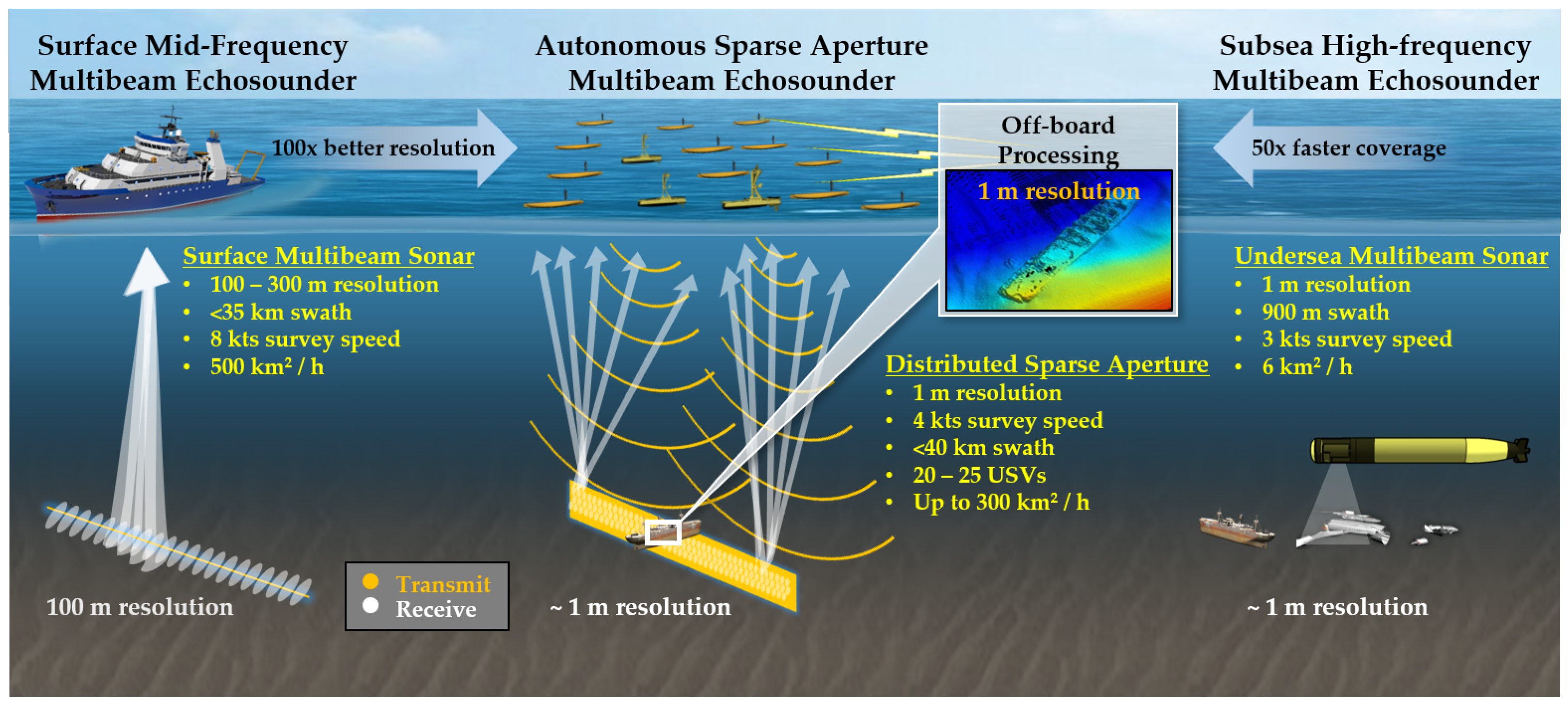
This work aims to develop and demonstrate a cost-effective technology for simultaneous high-resolution and rapid seafloor mapping in deep water. To generate comparable resolutions to the high-frequency systems that operate near the bottom of the ocean, a surface-based sonar must have an aperture approximately the size of those currently in use. However, the sonar arrays installed on existing large ocean mapping ships are already at the maximum size supported by their hulls [12,15]. To achieve a sonar array that is both cost-effective and larger than a ship hull, our design concept uses a small swarm of widely spaced ASVs, each hosting a small local sonar array, as shown in Figure 1.
In this concept, ASVs would work collaboratively to create a large effective array aperture, spanning hundreds of meters. However, for cost reasons, only a limited number of ASVs would be used to synthesize the array, on the order of tens of ASVs separated tens of meters from each other in a random pattern. With this sparse spatial sampling, the array achieves a lower signal-to-noise ratio (SNR) and is less able to reject noise coming from undesired directions because of high sidelobes [14]. However, these challenges can be mitigated using novel signal processing tools and acoustic propagation and imaging algorithms, including Bayesian and artificial intelligence (AI) schemes, enabling sparse arrays to achieve higher resolution. In addition, the ocean sound speed field needs to be estimated through the full water column, and the motions of the ASVs need to be measured very precisely. A surface-based sparse sonar system will need to be integrated with real-time, multiresolution probabilistic ocean field estimation, optimal ASV path planning and coordination, and Bayesian inversions and machine learning of ocean physics and acoustics fields [16,17,18,19].
Deploying several copies of this autonomous swarm of ASVs to map the deep ocean seabed at high resolution would enable data collection that could revolutionize our understanding and modeling of the ocean. The area coverage rate—estimated from sensor swath and survey speed—currently achievable for high-resolution mapping with an autonomous underwater vessel is approximately 6 km2/h, whereas a surface vessel maps at more than that rate, albeit only with low resolution. Efforts are underway to incrementally improve the efficiency of undersea-vehicle-based surveys—for instance, the recently developed PISCES system employs both surface and undersea sensors in a novel bistatic configuration [20]. Our system processes bistatic target reflections with a large sparse aperture operating from the surface and thus is capable of achieving a much greater coverage rate.
Autonomous systems enable cost-effective, extended-duration data collections that can map large areas of the deep ocean bottom. For a sparse-aperture system, the ocean field estimation, ASV path planning and coordination, Bayesian and AI inversions, and signal processing could be completed either onboard the ASVs or remotely. For example, the ASVs could be deployed from a ship, controlled and guided remotely, and left to map the seabed (including searching for a particular object on the seabed) for months until maintenance is needed. All collected data would be returned through a satellite link, and a high-resolution map of the seabed could be generated remotely.
The long-term goal is to demonstrate that a small swarm of ASVs can achieve high-resolution maps of the seabed from the ocean surface. This work addresses two specific objectives:
- To demonstrate that a sonar array composed of multiple collaborative ASVs can produce a high-resolution map of the seabed in deep water with precise relative positioning knowledge;
- To demonstrate that a single ASV working in conjunction with a large sonar array can achieve all position, timing, and acoustic signal requirements to work effectively as part of the large array.
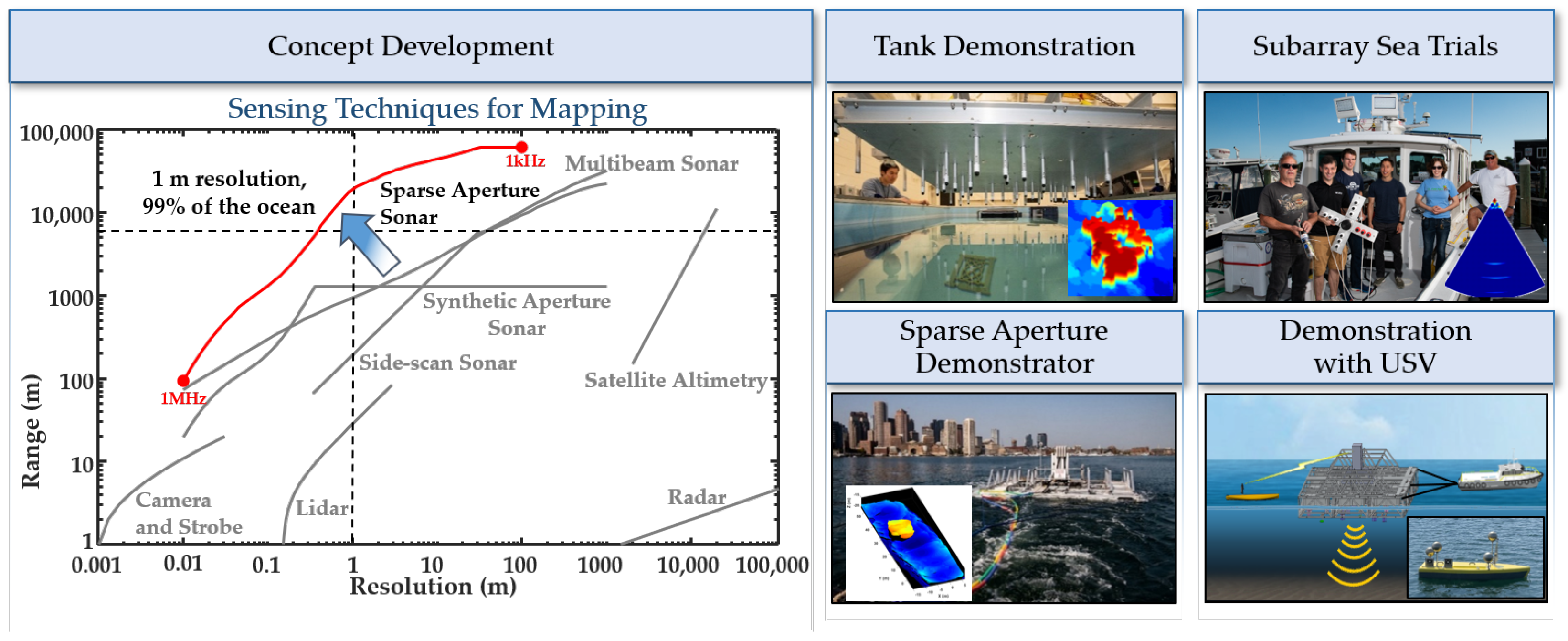
Our teams at the Lincoln Laboratory (LL) and Massachusetts Institute of Technology (MIT) have started working toward achieving these two goals. In particular, design studies and risk-reduction efforts for the overall project have been performed, including an analysis of the concept; a demonstration of a sparse aperture in a tank; the development of a low-cost, ASV-sized sonar array; sea testing of a large sonar array; the fabrication of a first-generation ASV; and initial relative navigation algorithm development. Figure 2 shows an overview of the technological development phases. This paper describes the design and specifications of our ocean floor mapping system and the techniques used for data acquisition, signal processing, and imaging. We illustrate the system’s capabilities using a proof-of-principle tank test at MIT LL Autonomous Systems Development Facility and an ocean test in Boston Harbor. Furthermore, we highlight our current efforts toward building an autonomous sparse-aperture sonar onboard multiple ASVs and precision-relative navigation system for the ASVs.
The rest of the article is organized as follows. In Section 2, we outline our system design and present the signal-processing chain and imaging algorithms used to obtain 3D seafloor maps. We provide validation results from a tank test using a proof-of-principle sonar in Section 3. In Section 4 and Section 5, we describe an application of our system in producing a 3D reconstruction of a sunken barge near Boston Harbor and current efforts to develop precision-relative navigation for ASVs, respectively. In Section 6, we discuss overall system design and performance, and our future project plans are provided in Section 7. Lastly, we discuss environmental impacts in Appendix A and outline our algorithm to reduce sidelobe effects in sparse array data in Appendix B.
2. System Overview
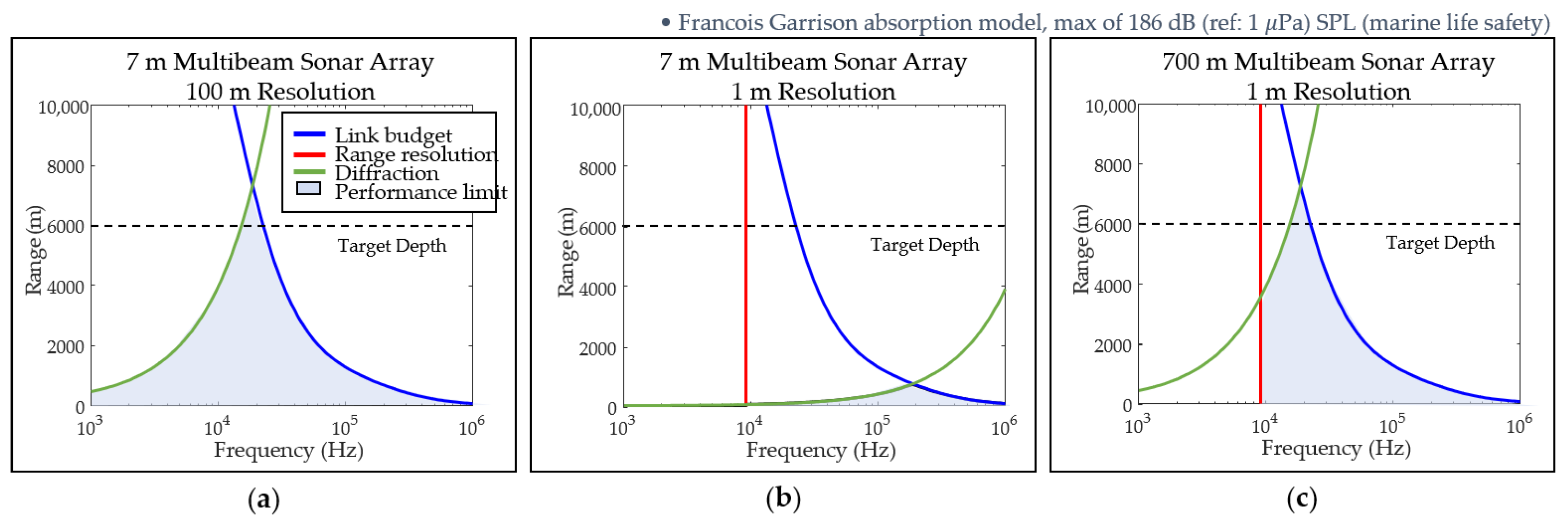
The motivation for developing a large acoustic aperture comes from trade-offs between imaging distance, resolution, operating frequency, and aperture size. To illustrate these trade-offs, consider three scenarios with different aperture sizes and resolution requirements. In Figure 3, the blue curves represent the link budget—the maximum imaging distance as a function of frequency given a maximum sound pressure level (186 dB re 1 μPa for marine life safety) and the minimum required SNR. This link budget limit does not change significantly in the three scenarios. The red and green curves are the range resolution and the diffraction limits for each system, respectively. To achieve 100× better range and cross-range resolution, the signal bandwidth needs to be wider and the wavelength needs to be shorter, so both limits shift to the right by two orders of magnitude.
The shaded areas indicate possible operating regions for the sonar systems. For instance, when operating near 20 kHz, a 7 m sonar array can achieve a 100 m resolution to at least the target depth of 6 km, a depth greater than 99% of the world’s oceans’ depths. However, to achieve 1 m resolution, the same sonar array can only reach slightly over 1 km. Therefore, the solution to higher resolution at longer distances is to increase the diffraction limit of the system without increasing frequency, thereby requiring the sonar aperture to be significantly increased. For example, a system using a 100× larger array can achieve a 1 m resolution while operating beyond the target depth of 6 km.
A larger sonar aperture increases the diffraction limit of the sonar and enables high-resolution imaging from longer ranges. Traditionally, sonar apertures are populated with transducers at half-wavelength spacing. For very large apertures, this approach would be prohibitive in terms of size, weight, power requirements, and cost. Therefore, we designed a large aperture sonar system with a sparsely populated 2D array of transmit and receive elements.
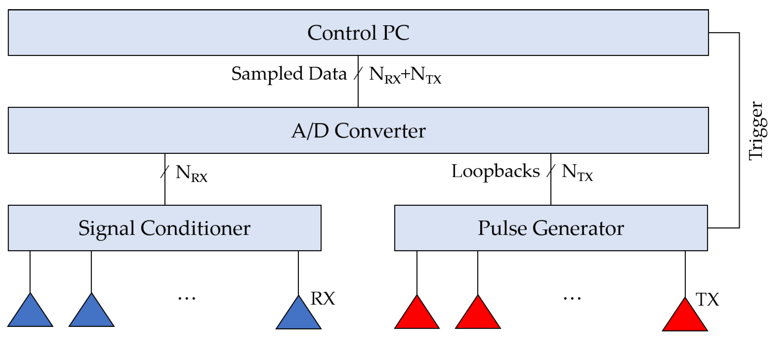
To demonstrate this concept, we implemented a sparse-aperture multiple-input, multiple-output (MIMO) sonar system that comprises pulse generators, a sparse transmit and receive array, multichannel signal conditioners, and signal converters, as shown in Figure 4. The pulse generators have calibration loopback outputs, which are used as a reference to compensate for time jitter and time drift. Receive elements have flat sensitivity over the operating frequency band. Signal conditioner consists of single-ended-to-differential converter for reducing the impact of common-mode noise pickup and harmonics, low-noise amplifiers for improving dynamic range and sensitivity, and anti-aliasing low-pass filter.
According to Huygens’ principle, combining radiated pulses from multiple transmitters to perform space-time focusing to improve array performance is possible [21]. However, this method requires transmitters to generate identical waveforms while maintaining precise positioning and time synchronization. Implementing such an approach for the distributed ASV array would significantly increase the cost and hardware complexity, so the concept of transmit focusing was not included in the current system design.
To achieve orthogonality with MIMO, we adopted a time-division multiple access (TDMA) transmission scheme in which transmitted waveforms share the same frequency band but at different time slots. During each time slot, a single transmitter insonifies the area under the array with a short pulse, and all sparse receive elements are used to sample the scattered wavefield. This sparse MIMO array significantly reduces the number of required transducers and cost but at the expense of less array gain and increased sidelobe level. Therefore, specialized signal processing and image reconstruction algorithms are needed to extract maximal information from the data and to optimize the sparse array performance.
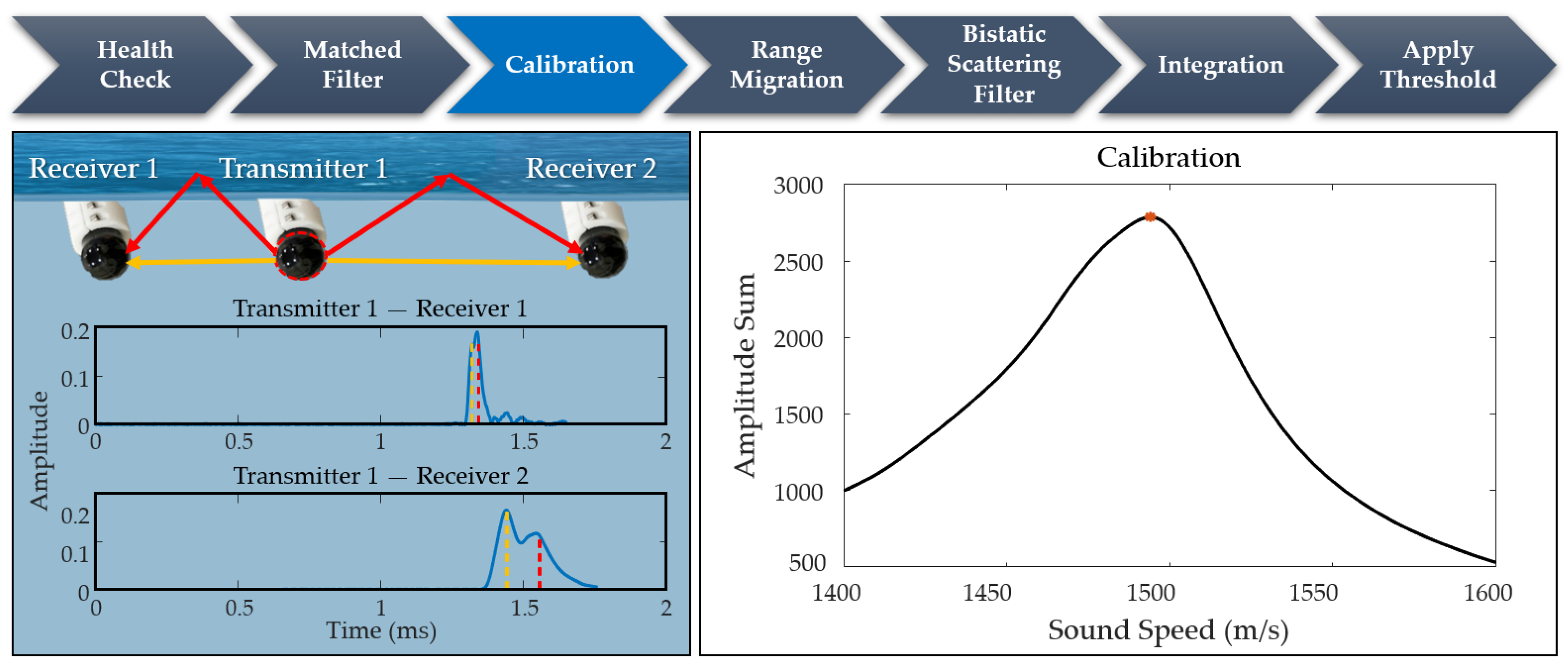
2.1. Signal-Processing Chain
A custom signal-processing chain was developed to condition the data for the image reconstruction step. The first step in the signal-processing chain is to check the health of all source transducers and receive hydrophones. Any sources that do not transmit or any dead or noisy transducers are excised, so they will not be included in the processing. The next step is to match the filter receiving data by convolving it with a replica of the transmitted pulse from each source. Matched filtering increases the temporal resolution of the data and improves the SNR by suppressing noise through coherent integration. Because the waveforms used in the ocean testing sonar system are generated on-demand in hardware and to provide information on the exact time of transmission, the transmitted signals are also recorded on separate loopback channels. The source transducers typically cannot transmit the full frequency extent of the generated waveforms (i.e., they have significant roll-off away from their peak resonant frequency), so a bandpass filter is also applied to suppress the artifact.
The final step of the signal-processing chain is calibrating the data, as shown in Figure 5, by time-aligning the data across receive channels and refining the estimates of array element locations and sound speed needed for image processing. Many hydrophones made up the sonar array used in the ocean testing, which required 12 separate 24-channel audio interfaces (i.e., analog-to-digital converters). Because of this requirement, slight timing differences can exist between channels connected to different audio interfaces. A broadband, pseudo-random noise signal was generated and injected into one channel on each audio interface. These channels were then used to estimate (using time correlation) and correct the relative time offsets between channels on different audio interfaces. The synchronized data were then used to refine the estimates of the transducer and hydrophone locations and the sound speed in the water. The refinement was completed using iterative optimization routines to maximize the total energy at each receiver after summing over the one-way (source-to-receiver or “direct path”) signal from all sources. These refined estimates are subsequently used to perform range migration in the image processing step.
2.2. Imaging Algorithms
Following geometry processing, data filtering, and calibration, the next step is to define a reconstruction grid underneath the array to cover the search area. We adopted range migration approach to construct the 3D image of the ocean floor because of the advantages this approach offers in computing a high-resolution image at a relatively low computation cost, making it well-suited for near real-time operations. Specifically, we implemented two popular imaging algorithms: diffraction stack [22] and Kirchhoff migration, which was first intuited in 1954 by Hagedoorn [23] and has been refined significantly since then for 2D and 3D applications in acoustic, seismic, and electromagnetic wave imaging [24,25,26]. Both imaging algorithms can be understood using the following example. If a point in our binning grid was located on the boundary of the object we are interested in imaging, as shown in Figure 6, then the outgoing wave from the transmitter reflects at that point and propagates back to one of the receivers. The pressure signal measured at the receiver will then have a maximum at an instant corresponding to the travel time from the transmitter to the voxel and back to the receiver. Integrating pressure measurements from all receivers at corresponding travel times will show a strong reflectivity value if a voxel lies on the object’s surface.
Because of our sparse aperture and the high-resolution requirements, the migrated image suffers from significant sidelobes. To address this limitation, we implemented scattering models to filter the reflected signals at each voxel. Our implementation included models for Lambert’s scattering [21], Phong diffuse and specular reflections [27], and the more general Ellis and Crowe bistatic scattering model [28], shown in Figure 6. The imaging and scattering algorithms were implemented for computation using MATLAB, which is a software package that can use graphics processing units to accelerate the computation. For instance, computing a high-resolution 3D image of a region on a grid (i.e., ∼50 million voxels at ∼1 mm resolution) takes around min on a NVIDIA RTX A6000 48 GB GDDR6 unit.
The last step in our approach corresponds to visualizing the migrated image. We use a box filter to integrate the energy in a small box of voxels into one larger, lower-resolution voxel, which helps reduce the SNR. In addition, we compare the amplitudes of the voxels and set a threshold for “filled” or “empty”; typically, we have been using 14–18 dB above the minimum energy to be considered material instead of water.
Altogether, the imaging algorithm can be summarized as follows:
- Range migration—fill the volume underneath the array with voxels and estimate bistatic travel times for each voxel, then sum the matched filter amplitudes at that voxel from all the transmit receiver combinations.
- Scattering filter—use the scattering angle to filter the return strengths in each voxel.
- Integration—sum a cube of voxels into one larger voxel, essentially taking or voxels and combing all the energy in those voxels into one larger, lower-resolution voxel.
- Thresholding—compare the amplitudes of the voxels and threshold for “filled” vs. “empty” voxels.
3. Sparse-Aperture Sonar: Scaled Tank Test
To demonstrate that a large sparse-aperture sonar could be made and the sidelobe issue could be mitigated by appropriate array design and signal processing, we built a proof-of-principle sonar in a test tank. The sonar consists of 43 transducers that operate at 200 kHz across a 1.5 m aperture. The array is effectively 200 wavelengths in each direction, and with only 43 transducers, it is very sparse. Figure 7 shows a picture of the sparse sonar array above the test tank and example imagery.
In preparation for the oceangoing system, given that acoustic projectors are significantly more expensive than hydrophones (∼20× more), the system was biased toward many “receive” channels and few “transmit” channels. All beamforming and timing are performed on the receive side. The system has a custom data acquisition system that samples at 1.67 Msps, and all transmitters have loopbacks.
To generate the imagery from the acoustic data collected in the tank, we employed our custom signal-processing chain and imaging algorithms presented in Section 2. Figure 7 shows sample imagery of a 10 cm MIT LL logo positioned 10 cm above the tank bottom. The features of the logo are about 9 mm wide, and the acoustic wavelength is about 8 mm, so resolving the finer details of the logo is not expected. However, the overall extent is readily apparent.
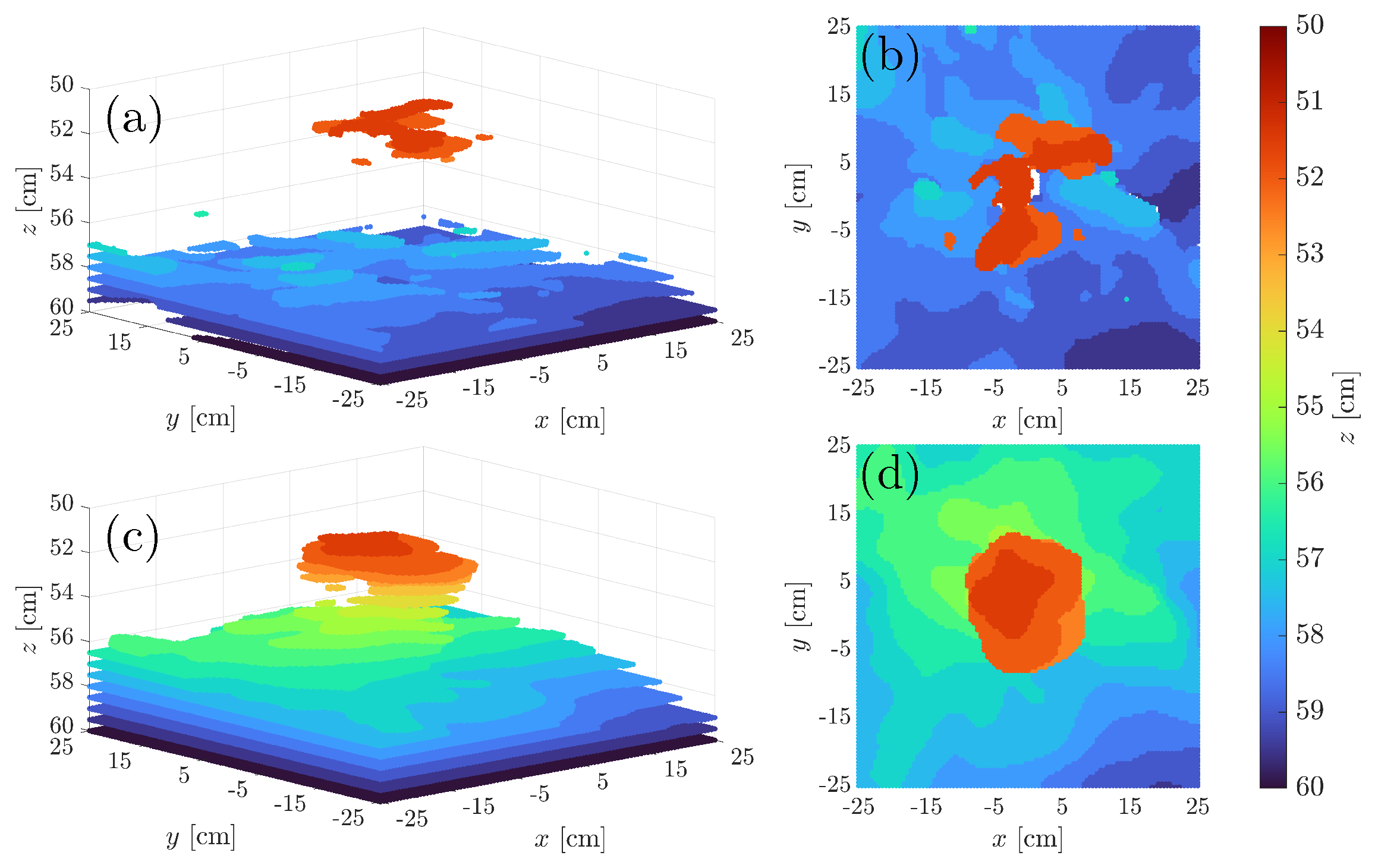
The imaging algorithms were compared to attain the sharpest image. Because of the vast volume of 3D, high-resolution data to be processed and limited computing power, we sought an algorithm that produced suitable images at the minimum possible computational expense. In each of the following cases, after processing the data, we set data thresholds such that voxels with energy less than dB of the maximum are treated as noise and not shown. We started by comparing the two different algorithms referenced in Section 2.2 in Figure 8: Kirchhoff migration and diffraction stack imaging. We used 0.5 cm resolution for this experiment and smoothed the data with a box filter. For Kirchhoff migration and diffraction stack imaging, we set and dB, respectively. Because Kirchhoff migration incorporates angular information, it produced far superior results to the diffraction stack.
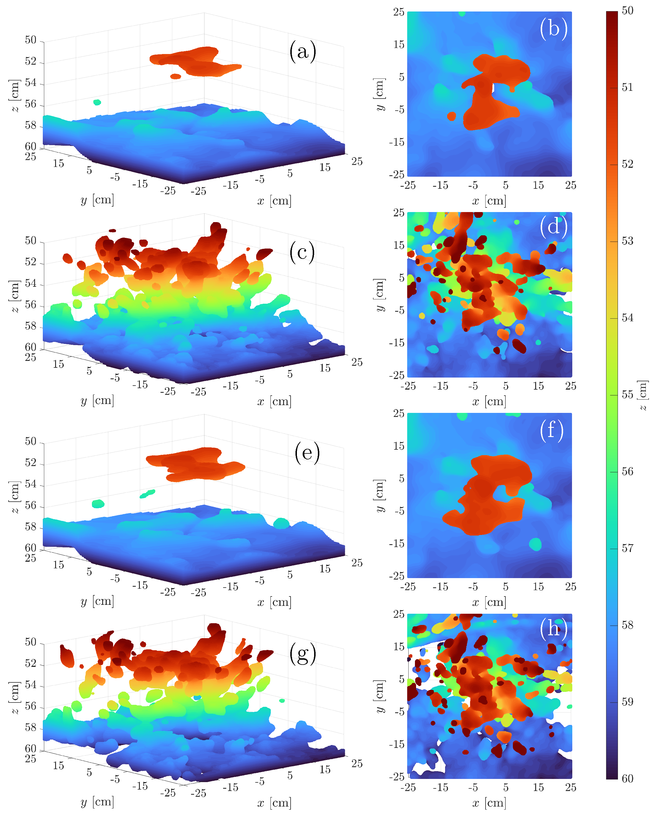
Next, we considered the different scattering models discussed in Section 2.2. We processed the data using Ellis’ and Crowe’s [28], Lambert’s [21], and Phong’s [27] scattering models, in addition to not using any scattering model at all with thresholds , and dB, respectively. In this experiment, we used a 0.1 cm resolution with a box filter to give an equivalent smoothed volume. Figure 9 shows the results of each scattering model. The Ellis and Crowe bistatic model and Phong model outperform the others; however, we note that the scattering models have tunable parameters, and Lambert model results for the tank data can improve with further optimization. Nevertheless, this experiment demonstrates the importance of an appropriate scattering model in 3D imaging.
Finally, using the Ellis and Crowe bistatic scattering model, we determined at what resolution to process the data. Our goal was to find the minimum resolution such that no discernible details were lost. In Figure 10, we compared 1 cm, 0.5 cm, 0.1 cm, and 0.05 cm resolutions with dB. In contrast to the previous examples, we did not use a box filter so that none of the fine details in the image would be removed. We find that the 0.1 cm and 0.05 cm images produce similar results. However, voids in imagery start to appear with a coarser resolution setting. At a frequency of 200 kHz and assuming the sound speed of the water is 1500 meters per second, the wavelength of the sound emitted is 0.75 cm. The Nyquist criterion then dictates that we sample at least at a resolution of 0.375 cm. This analysis aligns with our experiment, as 0.1 cm is the maximum voxel size tested that satisfies this criterion and the resolution at which we see the most image details.
4. Sparse-Aperture Sonar: Ocean Test
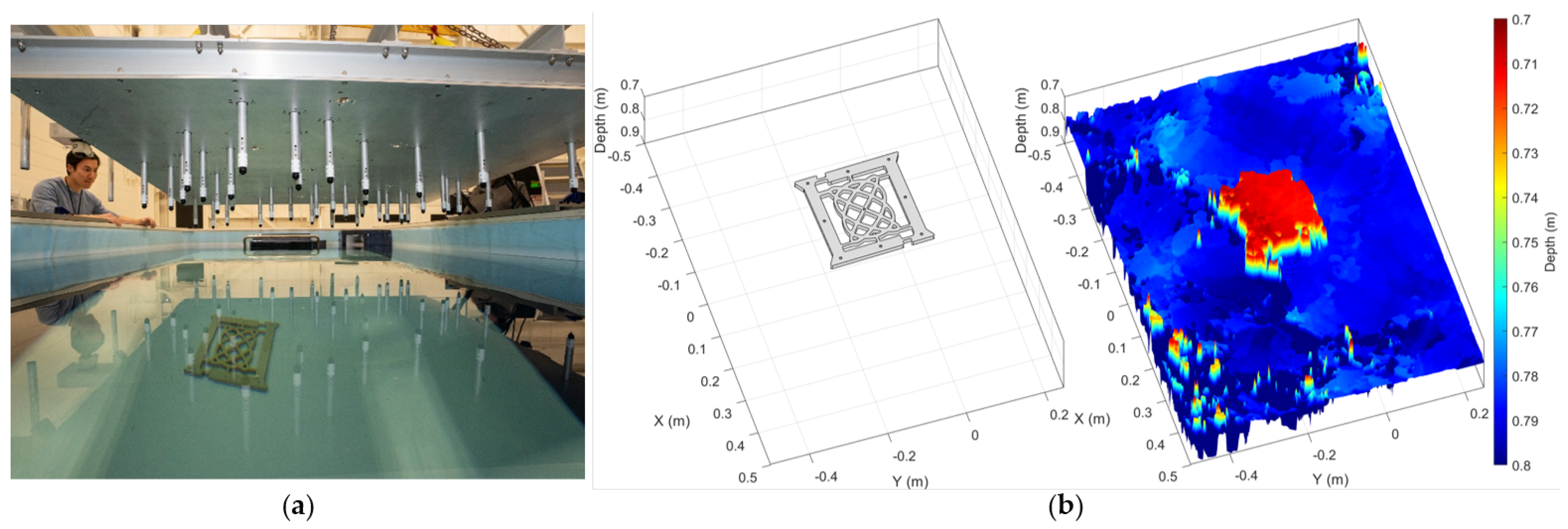
The tank testing shows that the sparse-aperture concept itself is viable. However, tank experiments cannot fully simulate the ocean’s complex and dynamic acoustic propagation conditions and the relative position variations in distributed arrays resulting from ocean waves and currents. To address the former, we built an oceangoing large sparse-aperture sonar testbed, shown in Figure 11. The metal frame ensures that the hydrophones and transmitters are locked in position and that the array geometry varies by less than a tenth of the wavelength (4 mm), even in rough seas.
The frame holds together a sparse array of 6 transmitters and 19 cross-shaped receiving subarrays (with a total of 247 hydrophones). The frame also includes two inertial measurement units and a waterproof server rack that houses the data acquisition system with signal conditioners, signal converters, pulse generators for transmitters, and control PCs. All the sensors and electronics are remotely controllable via Ethernet. When assembled, the array is 8 m × 8 m (24′ × 24′), but it can be separated into three units to fit onto a single 53′ flatbed trailer. The system operates at 33 kHz and is designed for an initial operating depth of 150 m. Figure 12 shows the sparse array layout, range profiles of all transmitter–receiver pairs, and a bathymetry point cloud from pier-side sensor data acquisition testing and validation.
We identified sunken objects near Boston Harbor to image with our sonar array for an initial at-sea demonstration of the sparse-aperture concept. We installed a reference fathometer and ran Humminbird HELIX 7 side-scan sonar to generate reference imagery of the seabed. This side-scan sonar operates at 462 kHz and has a maximum range of 60 m. With 14× the operating frequency of our sparse array, the side-scan sonar is better equipped to resolve small features. Figure 13 shows the reference side-scan imagery and the imagery generated from our sparse sonar array of a sunken barge outside Boston Harbor. The sparse sonar array operates as a multibeam sonar. It can produce a full 3D reconstruction of the seabed, whereas the side scan generates an intensity versus range plot with narrow strips. Because of this difference in image formation techniques, a direct comparison of the two outputs is difficult. Qualitatively, however, the image resolution we are obtaining from our array is similar to that of the side-scan system. A more capable reference multibeam system will be used for further validation and quantitative comparison of the resolution.
5. Toward Autonomous Sparse-Aperture Sonar
As we have shown that sparse-aperture imaging of the seabed is possible, we are working to disaggregate the sonar array onto multiple ASVs. The first step is to derive the required position knowledge for all the hydrophones in the array to generate sharp and focused imagery. This position knowledge will serve as a requirement for how well each of the ASVs needs to be tracked. Using our tank demonstration sonar array, we confirmed that if we know the positions of all elements to one-tenth of the acoustic wavelength, we can generate clear imagery. Using our ocean data at 33 kHz and additional modeling, we can estimate the array’s performance degradation with element position error.
For example, the wavelength at 33 kHz is 4.5 cm, and from the tank experiments, we would expect sharply focused imagery with a 4.5 mm or less element position error. The power loss with simulated position errors at 33 kHz is shown in Figure 14. We see minimal degradation through the one-tenth wavelength uncertainty and a less than 0.5 dB loss. The 3 dB loss point is around 8 mm, or about one-sixth of a wavelength, and at about one-third of a wavelength, the performance drops precipitously. Therefore, the required position accuracy for hydrophones on the first-generation ASV will be one-tenth of a wavelength, 5 mm, the hope is to develop autofocus techniques to relax this requirement to one-third or one-fifth of a wavelength and reduce the cost of the ASVs.
We are working to demonstrate a low-cost, precision-relative navigation capability to achieve 5 mm, 3D relative position accuracy. We performed a trade study evaluating many potential relative navigation options: (1) GPS, (2) inertial measurement, (3) optical tracking, (4) LiDAR, (5) radio-frequency ranging, and (6) high-frequency (automotive) radar. The key performance parameters are sensor field of view, maximum range, measurement accuracy, and cost. We plan to use a fused GPS and inertial measurement with optical and LiDAR tracking. The stereo-optical measurements can be used to generate the most accurate relative measurements; however, this approach requires many cameras and targets, which may exceed cost constraints. LiDAR has excellent coverage and good potential solution accuracy. Figure 15 shows an example of a “dummy” ASV in a tank with GPS and inertial measurements onboard and offboard tracking with an optical sensor and LiDAR. Our current optical system post-processing can measure optical-marker rigid-body edge distances and interior angles with accuracies of 0.33 cm and 0.25°, respectively.
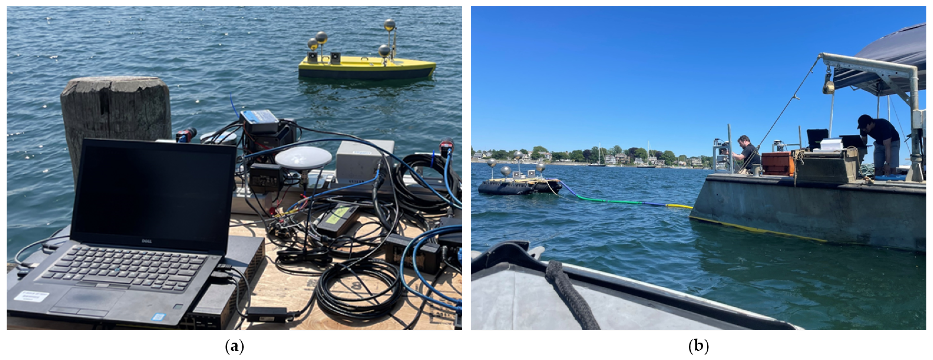
In collaboration with the Woods Hole Oceanographic Institution, we designed a low-cost ASV with a sonar array on the bottom that could have fiducials installed to enable precision tracking. The first of these ASVs has just been deployed and includes a 21-element passive sonar array, fully autonomous control, fused inertial navigation and GPS, and rigid markers for tracking. Pictures from the sea tests are shown in Figure 16. Optical markers are tracked using stereo cameras and LiDARs to generate precise 6-degrees-of-freedom relative poses of the ASVs.
6. Discussion: Overall System Design and Performance
In Section 3, we validated our ocean mapping system using a proof-of-principle sonar test in a scaled tank. The tank testing showed that the sparse-aperture concept is viable despite the challenges posed by the tank size causing significant signal interference and multipath effects. We also showcased the application of our imaging algorithms and showed the convergence of reconstructed images as we varied resolution. We compared the reconstructed images from the three scattering models and concluded that the Ellis and Crowe bistatic model provided the best results.
After demonstrating that the sparse-aperture concept is viable, in Section 4 we showcased the application of our system in reconstructing a 3D image of a sunken barge near Boston Harbor. We discussed details of our signal-processing and calibration chain and compared the image we obtained of the barge to that obtained by a commercial side-scan sonar. It should be noted that the imagery from our array was created using an initial algorithm set based on the signal-processing chain we developed for our tank experiment. Many aspects of the signal-processing suite would improve the quality of the imagery. Some of the possible improvements we are currently working on are listed in Table 1. In Appendix A, we discuss environmental impacts and how they can be expected to be limited compared to other systems.
A sparse array design introduces higher sidelobes than a fully populated dense array of equal size. A high sidelobe allows acoustic energy from other directions to smear into the look location of the array and degrades the image quality. In Appendix B, we showcase such sidelobe effects and outline our algorithm to reduce them. Specifically, Figure A2 and Figure A3 first confirm that a long inter-array distance introduces high sidelobe artifacts. Figure A4 shows that these sidelobe artifacts intensify for a spotlight-shaped transmit beam. This wide transmit beam illuminates a broader 2D patch of the seafloor than a 1D seafloor strip illumination from a narrow fan-shaped transmit beam and introduces more sidelobe energy leakage. We have developed a coherent sidelobe-reduction algorithm based on alternative projection [14] and the CLEAN algorithm of Hogbom [29]. Our algorithm effectively reduces sidelobe artifacts for a modeled Lambertian seafloor example, as shown in Figure A5. This algorithm is currently under further development, and we are planning performance analyses on both simulated scenarios and real measurements.
On the basis of our current ASV design, tracking system, and acoustic imaging, we have estimated the performance and costs of a fully operational array. Desired resolution of the seabed imagery determines the sonar operating frequency and the number and quality of navigation sensors needed to achieve the one-tenth-wavelength relative positioning accuracy. The accuracy requirement can be relaxed to one-third-wavelength with an autofocus mapping capability.
A conventional deep-water multibeam sonar has about 1° beam and costs around USD 2 million. The sparse array technique will require long-endurance ASVs that cost about USD 75,000 each. At 1 m resolution, using our current GNSS–visual–inertial navigation setup will require installing a precision GNSS receiver capable of real-time kinematics (RTK), inertial measurement unit, and multiple cameras and LiDARs on vehicles. The total cost of the system will be USD 7 million At lesser resolution requirements, such as 10 m, fewer ASVs are needed, and each vehicle can be outfitted with a less exquisite navigation sensor suite. The total cost drops to USD 2 million. An overview of this trade is shown in Figure 17, which shows the Pareto front of cost and resolution for the operational system.
7. Future Work
We plan to improve signal-processing and 3D image reconstruction algorithms by incorporating autofocus methods. We could also investigate merging these advances with our Bayesian uncertainty quantification and learning using our dynamically orthogonal stochastic acoustic wave predictions [30,31]. A key aspect of the planned sea tests is the prediction of the ocean fields (e.g., sound speed, currents) to be used in estimating the bathymetry and seabed properties from the acoustic data and some temperature, salinity, and biogeochemical data. We could employ our MIT Multidisciplinary Simulation, Estimation, and Assimilation System (MSEAS) ocean modeling system [32,33], optimal reduced-order theory and schemes for uncertainty quantification, and Bayesian data assimilation and learning [34,35]. We could first predict joint probability density functions (PDFs) of the uncertain ocean and seabed fields, using our new coupled dynamically orthogonal stochastic ocean acoustic partial differential equations [36,37,38,39], with extension to multiresolution probabilistic predictions. With these prior PDFs, our Bayesian inference algorithms then assimilate the measured acoustic data and sound speed profiles to jointly estimate posterior PDFs for the ocean fields, bathymetry, and seabed’s geoacoustic properties [36,40]. With Bayesian and machine learning [41,42], we can then jointly learn better parameterizations (e.g., for scattering), neural model closures (e.g., for missing or unknown model terms), and even model formulations themselves (e.g., for model complexity).
For the control and coordination of the ASVs, we could utilize our principled optimal path planning and coordination for operations in strong dynamic ocean currents and waves (e.g., [19,43,44]). With this model-based predictive control and path planning coordination, we could guide the ASV headings and speeds to ensure that the ASV remains in an optimal location with respect to the rest of the array. For multiple ASVs, our rigorous path planning and coordination methods could help maintain larger-scale patterns that are optimal for the inference of bathymetry while accounting for ocean currents and waves.
Author Contributions
Conceptualization and methodology, P.R., A.M. and P.F.J.L.; software, P.R., K.A., B.C., A.M., W.H.A. and A.C.; investigation and data curation, P.R., D.B. and A.M.; writing—original draft preparation and writing—review and editing, all authors; supervision and project administration, A.M. and P.F.J.L. All authors have read and agreed to the published version of the manuscript.
Funding
This research is supported by the Under Secretary of Defense for Research and Engineering under Air Force Contract No. FA8702-15-D-0001. Any opinions, findings, conclusions or recommendations expressed in this material are those of the authors and do not necessarily reflect the views of the Under Secretary of Defense for Research and Engineering.
Institutional Review Board Statement
Not applicable.
Informed Consent Statement
Not applicable.
Data Availability Statement
The data presented in this study are available on request from the corresponding authors.
Acknowledgments
We thank Katherine Rimpau of MIT Lincoln Laboratory for assistance with data acquisition and data analysis, Paul Pepin of MIT Lincoln Laboratory for exceptional design of the apparatuses, and our colleagues on the MIT Lincoln Laboratory Autonomous Systems Line and Integrated Systems Line Committees for their helpful technical advice.
Conflicts of Interest
The authors declare no conflict of interest.
Appendix A. Environmental Impacts
The only foreseen potential environmental impact of this system is the acoustic effects on marine life. A typical multibeam echosounder on a surface ship designed for deep water produces a 240 dBuPA@1m sound pressure level (SPL) and has a wide beam of around 140°. Given the expense of ship operations, the sonar is run continuously. Our current rigid sonar array is intentionally power limited such that it does not require permitting to use. The acoustic projectors are standard commercial fathometers modified to play alternative waveforms at reduced maximum output power. They also have a very narrow, 22°, downward-pointing beam. Using 160 dB SPL criteria for Level B harassment, a marine mammal within 10,000 m of the ship would be behaviorally harassed. However, with our current array, a marine mammal would need to be within 8 m and 11° off-vertical from our transducer to be behaviorally harassed. An animal must be underneath the array and within 8 m to be affected by our testing. Overall, the environmental impact of the prototype sparse-aperture array is less than that of other vessel traffic employing a low-frequency fathometer.
For a future operational system using ASVs, the beam width of the transmitters and power level will be increased. The power level will still be less than that of a surface ship multibeam. To mitigate the increase in SPL and beam width, we intend to develop an automated detector of marine mammal sounds and pause testing when marine mammals are suspected to be in the vicinity of the array. The testing pause is much less impactful for an autonomous system than for a large capital ship. Figure A1 compares the rough areas underneath a conventional multibeam, our existing array, and a future potential sparse-aperture operational system in which a marine mammal may be harassed.
Figure A1.
Approximate distance from acoustic sources that exceed 160 dB sound pressure level for a typical ship-based multibeam echosounder, our existing prototype array, and a future first-generation operational system.
Figure A1.
Approximate distance from acoustic sources that exceed 160 dB sound pressure level for a typical ship-based multibeam echosounder, our existing prototype array, and a future first-generation operational system.

Appendix B. High Sidelobe Effects in a Sparse Array Image and Reduction Algorithm Development
This section shows the sidelobe effects in a sparse array image and investigates their cause. We also briefly introduce a potential sidelobe reduction algorithm and demonstrate its effectiveness by simulation.
Appendix B.1. High Sidelobe Effects in a Sparse Array Image
Here, we simulate the sidelobe effects in a sparse array image and compare it with a dense-array image. Figure A2 and Figure A3 show that a sparse array leads to more sidelobe artifacts and degrades the image quality. This outcome is due to sidelobe energy from other seafloor pixels smearing into the array’s look position.
A 2D seafloor further degrades image quality, as shown in Figure A3 and Figure A4. A 1D seafloor strip effectively models a fan-shaped transmit beam wide in one horizontal direction and narrow in the other (Figure A3). A 2D seafloor patch models a spotlight-shaped transmit beam wide in both horizontal directions (Figure A4). This spotlight-shaped transmit beam illuminates a relatively wide area of the seafloor and increases energy smearing from the seafloor around the array’s look location.
Figure A2.
A simulated 1D Lambertian seafloor strip imaged by a dense uniform line receive array. A 0.05 s linear frequency-modulated transmit waveform at kHz is projected from a transmit element at the center of the receive array. The received signal at each receive element is matched filtered and then beam-formed for each spatial voxel position. Scattered energy is well-contained within the seafloor region. No random ambient noise is used.

Figure A3.
Simulated imaging with a sparse array. The environmental configuration and transmit waveform are the same as those in Figure A2. The geometry of the sparse receive array and the transmitter is shown. The matched filtered and beamforming scattered output energy is spread around the seafloor region because of the sidelobes. Note that a 1D bottom strip models a fan-shaped transmit beam that is narrow in the x direction and wide in the y direction.

Figure A4.
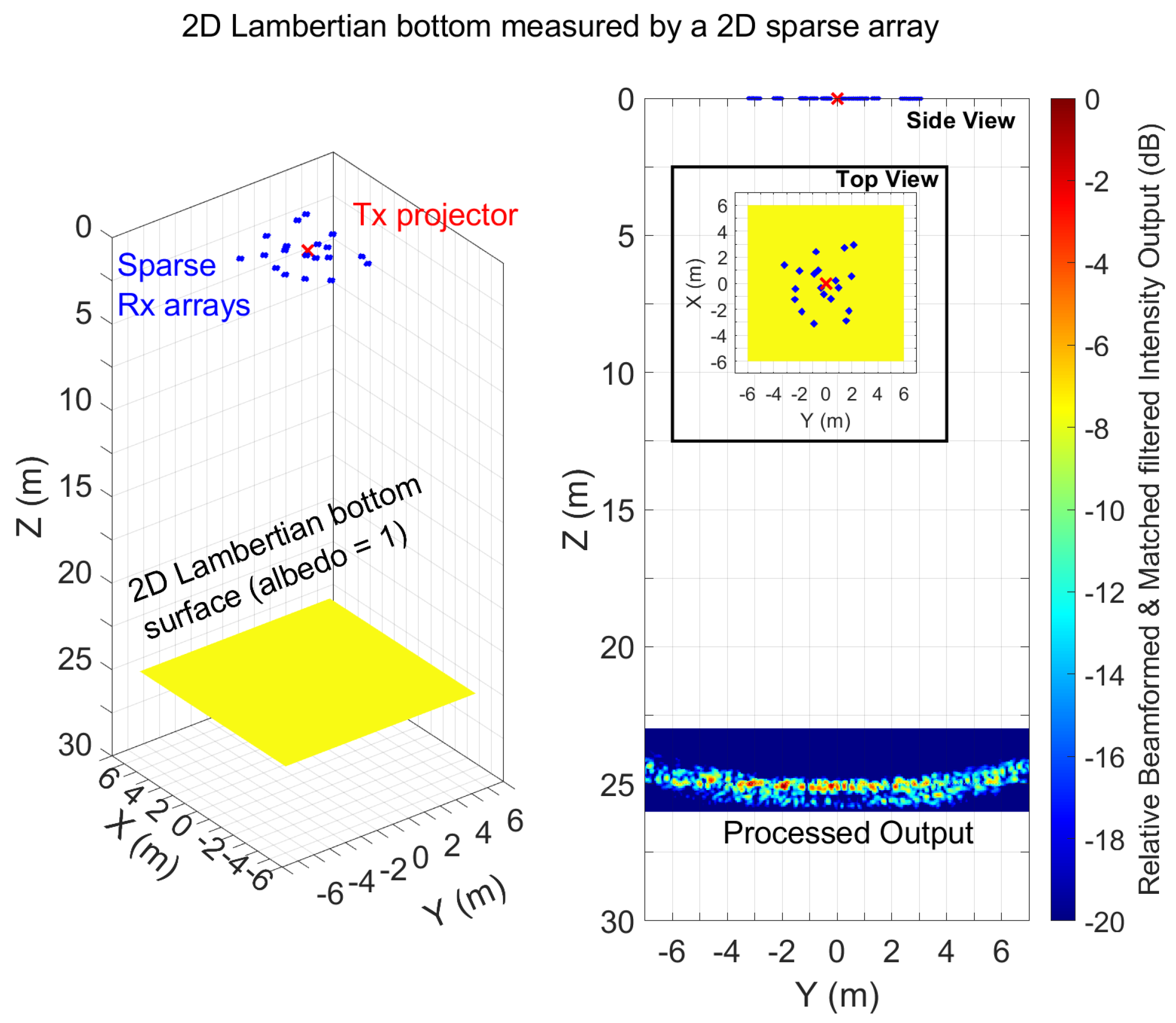
A simulated sparse array image of a 2D Lambertian seafloor. The array configurations are the same as those in Figure A3. A 2D seafloor effectively represents a spotlight-shaped transmit beam that is wide in both x and y directions. The 2D seafloor scattering increases sidelobe artifacts and further degrades image quality.
Figure A4.
A simulated sparse array image of a 2D Lambertian seafloor. The array configurations are the same as those in Figure A3. A 2D seafloor effectively represents a spotlight-shaped transmit beam that is wide in both x and y directions. The 2D seafloor scattering increases sidelobe artifacts and further degrades image quality.

Appendix B.2. Sidelobe-Reduction Algorithm Development
We are developing algorithms to reduce sidelobe artifacts and improve image quality. We briefly describe the present algorithm and demonstrate its performance for a simple simulated case.
Our algorithm shares a similar philosophy with the alternative projection [14] that is widely used in passive sonar applications. Both algorithms estimate a single-point source and its waveform at each iteration. Alternative projection estimates the signal waveform of a point source as the entire component contained in its estimated direction. Estimating the waveform with a single step can cause energy smearing from nearby sources. Imaging a cluttered region with a sparse array system with typically high sidelobe levels can suffer from energy smearing from other sources or background noise and severely contaminate the waveform estimate. Our algorithm partially estimates the underlying point source’s waveform at each iteration. The estimation is less susceptible to contamination by other point sources or background noise, as sidelobe leakage from neighboring sources also decreases as iterations progress.
The iterative scheme we implement is inspired by the CLEAN algorithm of Hogbom [29], which is commonly used for long-baseline astronomical interferometry. However, our deconvolution algorithm is different from the original CLEAN algorithm. The CLEAN algorithm was originally developed based on the van Certtite–Zernike theorem [45,46]. It uses the duality property of the cross-correlation of the electric field measured at two distinct points, i.e., visibility and directional spectral density. The CLEAN algorithm operates on the second-moment statistics and removes sidelobe power artifacts. Our algorithm uses the direct acoustic pressure field and estimates the location and waveform of underlying point sources to remove the sidelobe field artifacts.
Our algorithm starts with matched filtering, followed by beamforming the received signal. This coherent processing is typically performed in the complex baseband for computational efficiency, and, as a result, the raw processed outputs are also complex values. The order of matched filtering and beamforming are interchangeable because both processes are linear. It is, however, computationally efficient to first matched filter the element time series when the number of voxels exceeds the number of “receive” elements. We define the raw complex output of the coherent processing as the “complex dirty map”, following the terminology in the original CLEAN algorithm [29]. The algorithm then finds the power peak location in the dirty map and calculates the complex point response function at that peak location. The complex point response function is defined as the “complex dirty beam”. The peak height of the complex dirty beam is scaled by 10–25% of the dirty map power peak strength with a phase identical to the complex dirty map peak. This scaled, phase-shifted complex point source at the detected peak position is added to an empty spatial map and forms the “complex clean map”. A “complex residual map” is also calculated by subtracting the complex dirty beam of this point source from the initial dirty map. Our algorithm repeats the same procedure, except the updated complex residual map is used instead of the complex dirty map to detect the power peak in consecutive iterations. Iteration continues until the peak power in the complex residual map falls below a desired level—for example, 30 dB below the peak power of the original complex dirty map.
Figure A5.
Example of a sidelobe-reduction algorithm for a simulated 1D Lambertian seafloor. The environmental and array configurations are the same as those in Figure A3. The estimated point source locations are well contained within the seafloor region, as shown by the final clean map after 1000 iterations.

References
- Rengstorf, A.M.; Mohn, C.; Brown, C.; Wisz, M.S.; Grehan, A.J. Predicting the distribution of deep-sea vulnerable marine ecosystems using high-resolution data: Considerations and novel approaches. Deep Sea Res. Part Oceanogr. Res. Pap. 2014, 93, 72–82. [Google Scholar] [CrossRef]
- Picard, K.; Brooke, B.P.; Harris, P.T.; Siwabessy, P.J.; Coffin, M.F.; Tran, M.; Spinoccia, M.; Weales, J.; Macmillan-Lawler, M.; Sullivan, J. Malaysia Airlines flight MH370 search data reveal geomorphology and seafloor processes in the remote southeast Indian Ocean. Mar. Geol. 2018, 395, 301–319. [Google Scholar] [CrossRef]
- Chiocci, F.L.; Cattaneo, A.; Urgeles, R. Seafloor mapping for geohazard assessment: State of the art. Mar. Geophys. Res. 2011, 32, 1–11. [Google Scholar] [CrossRef] [Green Version]
- Picard, K.; Tran, M.; Siwabessy, P.J.; Kennedy, P.; Smith, W. Increased resolution bathymetry in the southeast Indian ocean: MH370 search data. Hydro Int. 2017, 21, 14–19. [Google Scholar]
- Kearns, T.A.; Breman, J. Bathymetry—The art and science of seafloor modeling for modern applications. Ocean Globe 2010, 1–36. [Google Scholar]
- Levin, L.A.; Bett, B.J.; Gates, A.R.; Heimbach, P.; Howe, B.M.; Janssen, F.; McCurdy, A.; Ruhl, H.A.; Snelgrove, P.; Stocks, K.I.; et al. Global Observing Needs in the Deep Ocean. Front. Mar. Sci. 2019, 6, 241. [Google Scholar] [CrossRef]
- Wölfl, A.C.; Snaith, H.; Amirebrahimi, S.; Devey, C.W.; Dorschel, B.; Ferrini, V.; Huvenne, V.A.I.; Jakobsson, M.; Jencks, J.; Johnston, G.; et al. Seafloor Mapping—The Challenge of a Truly Global Ocean Bathymetry. Front. Mar. Sci. 2019, 6, 283. [Google Scholar] [CrossRef] [Green Version]
- Hansen, R.E.; Callow, H.J.; Sabo, T.O.; Synnes, S.A.V. Challenges in seafloor imaging and mapping with synthetic aperture sonar. IEEE Trans. Geosci. Remote Sens. 2011, 49, 3677–3687. [Google Scholar] [CrossRef]
- Jalving, B. Depth accuracy in seabed mapping with underwater vehicles. In Proceedings of the Oceans ′99—Riding the Crest into the 21st Century, Conference and Exhibition, Conference Proceedings (IEEE Cat. No.99CH37008). Seattle, WA, USA, 13–16 September 1999; Volume 2, pp. 973–978. [Google Scholar]
- Wynn, R.B.; Huvenne, V.A.; Le Bas, T.P.; Murton, B.J.; Connelly, D.P.; Bett, B.J.; Ruhl, H.A.; Morris, K.J.; Peakall, J.; Parsons, D.R.; et al. Autonomous Underwater Vehicles (AUVs): Their past, present and future contributions to the advancement of marine geoscience. Mar. Geol. 2014, 352, 451–468. [Google Scholar] [CrossRef] [Green Version]
- Lucieer, V.L.; Forrest, A.L. Emerging mapping techniques for autonomous underwater vehicles (AUVs). In Seafloor Mapping Along Continental Shelves; Springer: Berlin/Heidelberg, Germany, 2016; pp. 53–67. [Google Scholar]
- Mayer, L.; Jakobsson, M.; Allen, G.; Dorschel, B.; Falconer, R.; Ferrini, V.; Lamarche, G.; Snaith, H.; Weatherall, P. The Nippon Foundation GEBCO seabed 2030 project: The quest to see the world’s oceans completely mapped by 2030. Geosciences 2018, 8, 63. [Google Scholar] [CrossRef] [Green Version]
- Jakobsson, M.; Allen, G.; Carbotte, S.; Falconer, R.; Ferrini, V.; Marks, K.; Mayer, L.; Rovere, M.; Schmitt, T.; Weatherall, P.; et al. The Nippon Foundation GEBCO Seabed 2030: Roadmap for Future Ocean Floor Mapping. 2017. The Nippon Foundation GEBCO. Available online: https://seabed2030.gebco.net/documents/seabed2030 (accessed on 6 March 2023).
- Van Trees, H.L. Optimum Array Processing: Part IV of Detection, Estimation, and Modulation Theory; John Wiley & Sons: Hoboken, NJ, USA, 2004. [Google Scholar]
- Mayer, L.A. Frontiers in seafloor mapping and visualization. Mar. Geophys. Res. 2006, 27, 7–17. [Google Scholar] [CrossRef]
- Robinson, A.R.; Lermusiaux, P.F.J. Prediction Systems with Data Assimilation for Coupled Ocean Science and Ocean Acoustics. In Proceedings of the Sixth International Conference on Theoretical and Computational Acoustics, Honolulu, HI, USA, 11–15 August 2003; Tolstoy, A., Teng, Y., Shang, E.C., Eds.; pp. 325–342. [Google Scholar]
- Lermusiaux, P.F.J.; Haley, P.J., Jr.; Yilmaz, N.K. Environmental prediction, path planning and adaptive sampling: Sensing and modeling for efficient ocean monitoring, management and pollution control. Sea Technol. 2007, 48, 35–38. [Google Scholar]
- Wang, D.; Lermusiaux, P.F.J.; Haley, P.J., Jr.; Eickstedt, D.; Leslie, W.G.; Schmidt, H. Acoustically focused adaptive sampling and on-board routing for marine rapid environmental assessment. J. Mar. Syst. 2009, 78, S393–S407. [Google Scholar] [CrossRef]
- Lermusiaux, P.F.J.; Subramani, D.N.; Lin, J.; Kulkarni, C.S.; Gupta, A.; Dutt, A.; Lolla, T.; Haley, P.J., Jr.; Ali, W.H.; Mirabito, C.; et al. A Future for Intelligent Autonomous Ocean Observing Systems. J. Mar. Res. 2017, 75, 765–813. [Google Scholar] [CrossRef]
- Cruz, N.; Abreu, N.; Almeida, J.; Almeida, R.; Alves, J.; Dias, A.; Ferreira, B.; Ferreira, H.; Gonçalves, C.; Martins, A.; et al. Cooperative deep water seafloor mapping with heterogeneous robotic platforms. In Proceedings of the OCEANS 2017—Anchorage, Anchorage, AK, USA, 18–21 September 2017; pp. 1–7. [Google Scholar]
- Urick, R.J. Principles of Underwater Sound, 2nd ed.; McGraw–Hill: New York, NY, USA, 1975. [Google Scholar]
- French, W.S. Two-dimensional and three-dimensional migration of model-experiment reflection profiles. Geophysics 1974, 39, 265–277. [Google Scholar] [CrossRef]
- Hagedoorn, J.G. A process of seismic reflection interpretation. Geophys. Prospect. 1954, 2, 85–127. [Google Scholar] [CrossRef]
- Schneider, W.A. Integral Formulation for Migration in Two and Three Dimensions. Geophysics 1978, 43, 49–76. [Google Scholar] [CrossRef]
- Yilmaz, Ö. Seismic Data Analysis, 2nd ed.; Society of Exploration Geophysicists: Tulsa, OK, USA, 2001; Volume 1. [Google Scholar]
- Zhuge, X.; Savelyev, T.; Yarovoy, A.G.; Ligthart, L. UWB array-based radar imaging using modified Kirchhoff migration. In Proceedings of the 2008 IEEE International Conference on Ultra-Wideband, Hannover, Germany, 10–12 September 2008; Volume 3, pp. 175–178. [Google Scholar]
- Phong, B.T. Illumination for computer generated pictures. Commun. ACM 1975, 18, 311–317. [Google Scholar] [CrossRef] [Green Version]
- Ellis, D.D.; Crowe, D.V. Bistatic reverberation calculations using a three-dimensional scattering function. J. Acoust. Soc. Am. 1991, 89, 2207–2214. [Google Scholar] [CrossRef]
- Hogbom, J. Aperture synthesis with a non-regular distribution of interferometer baselines. Astron. Astrophys. Suppl. 1974, 15, 49. [Google Scholar]
- Charous, A.; Lermusiaux, P.F.J. Dynamically Orthogonal Runge–Kutta Schemes with Perturbative Retractions for the Dynamical Low-Rank Approximation. SIAM J. Sci. Comput. 2022; in press. [Google Scholar]
- Bhabra, M.S.; Lermusiaux, P.F.J. Stochastic Dynamically Orthogonal Acoustic Wavefront Equations; Massachusetts Institute of Technology: Cambridge, MA, USA, 2023; Manuscript in preparation. [Google Scholar]
- Haley, P.J., Jr.; Lermusiaux, P.F.J. Multiscale two-way embedding schemes for free-surface primitive equations in the “Multidisciplinary Simulation, Estimation and Assimilation System”. Ocean. Dyn. 2010, 60, 1497–1537. [Google Scholar] [CrossRef]
- Haley, P.J., Jr.; Agarwal, A.; Lermusiaux, P.F.J. Optimizing Velocities and Transports for Complex Coastal Regions and Archipelagos. Ocean. Model. 2015, 89, 1–28. [Google Scholar] [CrossRef] [Green Version]
- Lu, P.; Lermusiaux, P.F.J. Bayesian Learning of Stochastic Dynamical Models. Phys. Nonlinear Phenom. 2021, 427, 133003. [Google Scholar] [CrossRef]
- Subramani, D.; Lermusiaux, P.F.J. Probabilistic Ocean Predictions with Dynamically-Orthogonal Primitive Equations; Massachusetts Institute of Technology: Cambridge, MA, USA, 2023; Manuscript in preparation. [Google Scholar]
- Ali, W.H.; Bhabra, M.S.; Lermusiaux, P.F.J.; March, A.; Edwards, J.R.; Rimpau, K.; Ryu, P. Stochastic Oceanographic-Acoustic Prediction and Bayesian Inversion for Wide Area Ocean Floor Mapping. In Proceedings of the OCEANS 2019 MTS/IEEE SEATTLE, Seattle, WA, USA, 27–31 October 2019; pp. 1–10. [Google Scholar] [CrossRef]
- Ali, W.H.; Lermusiaux, P.F.J. Dynamically Orthogonal Narrow-Angle Parabolic Equations for Stochastic Underwater Sound Propagation. J. Acoust. Soc. Am. 2023; manuscript under review. [Google Scholar]
- Charous, A.; Lermusiaux, P.F.J. Dynamically Orthogonal Differential Equations for Stochastic and Deterministic Reduced-Order Modeling of Ocean Acoustic Wave Propagation. In Proceedings of the OCEANS 2021, San Diego, CA, USA, 20–23 September 2021; pp. 1–7. [Google Scholar] [CrossRef]
- Ali, W.H.; Lermusiaux, P.F.J. Dynamically Orthogonal Wide-Angle Parabolic Equations for Stochastic Underwater Sound Propagation; Massachusetts Institute of Technology: Cambridge, MA, USA, 2023; Manuscript in preparation. [Google Scholar]
- Ali, W.H.; Lermusiaux, P.F.J. Joint Ocean-Acoustic Inversion Using Gaussian Mixture Models and the Dynamically Orthogonal Parabolic Equations; Massachusetts Institute of Technology: Cambridge, MA, USA, 2023; Manuscript in preparation. [Google Scholar]
- Gupta, A.; Lermusiaux, P.F.J. Neural Closure Models for Dynamical Systems. Proc. R. Soc. 2021, 477, 1–29. [Google Scholar] [CrossRef]
- Gupta, A.; Lermusiaux, P.F.J. Bayesian Learning of Coupled Biogeochemical-Physical Models; Massachusetts Institute of Technology: Cambridge, MA, USA, 2023; Manuscript under review; Available online: https://arxiv.org/abs/2211.06714 (accessed on 6 March 2023).
- Lolla, T.; Haley, P.J., Jr.; Lermusiaux, P.F.J. Path planning in multiscale ocean flows: Coordination and dynamic obstacles. Ocean. Model. 2015, 94, 46–66. [Google Scholar] [CrossRef]
- Kulkarni, C.S.; Lermusiaux, P.F.J. Three-dimensional Time-Optimal Path Planning in the Ocean. Ocean. Model. 2020, 152, 101644. [Google Scholar] [CrossRef]
- van Cittert, P.H. Die wahrscheinliche Schwingungsverteilung in einer von einer Lichtquelle direkt oder mittels einer Linse beleuchteten Ebene. Physica 1934, 1, 201–210. [Google Scholar] [CrossRef]
- Zernike, F. The Concept of Degree of Coherence and Its Application to Optical Problems. Physica 1938, 5, 785–795. [Google Scholar] [CrossRef]
Figure 1.
The autonomous sparse-aperture concept offers a potential 100-fold improvement in resolution compared with existing surface ship multibeam sonar, or a potential 50-fold increase in coverage rate compared with subsea sonar.
Figure 1.
The autonomous sparse-aperture concept offers a potential 100-fold improvement in resolution compared with existing surface ship multibeam sonar, or a potential 50-fold increase in coverage rate compared with subsea sonar.

Figure 2.
Progression from concept development to sea testing of the sparse aperture.

Figure 3.
The performance-bound trade-off between imaging distance, resolution, frequency, and aperture. (a) A 7 m sonar array can achieve 100 m resolution at the target depth of 6 km. (b) A resolution of 1 m is possible, but the range is limited to 1 km. (c) A large 700 m aperture sonar can achieve 1 m resolution at the target depth and beyond.

Figure 4.
A block diagram of the sparse sonar data acquisition system for receivers (blue) and transmitters (red).
Figure 4.
A block diagram of the sparse sonar data acquisition system for receivers (blue) and transmitters (red).

Figure 5.
The calibration approach finds optimal sensor positions and sound speed by modeling direct path (orange) and surface bounce path (red) contributions in the matched filtered data (blue).
Figure 5.
The calibration approach finds optimal sensor positions and sound speed by modeling direct path (orange) and surface bounce path (red) contributions in the matched filtered data (blue).

Figure 6.
Illustrations of ray tracing in range migration, and the effect of varying the diffuse parameter () in Ellis and Crowe bistatic scattering filter application.
Figure 6.
Illustrations of ray tracing in range migration, and the effect of varying the diffuse parameter () in Ellis and Crowe bistatic scattering filter application.

Figure 7.
(a) The 200 kHz sparse aperture sonar array above the test tank and (b) CAD model of the target and acoustic reconstruction example.
Figure 7.
(a) The 200 kHz sparse aperture sonar array above the test tank and (b) CAD model of the target and acoustic reconstruction example.

Figure 8.
A comparison of the results of Kirchhoff migration (a,b) and diffraction stack (c,d) imaging, with (a,c) showing 3D visualizations and (b,d) showing a top-down view. Kirchhoff migration successfully localizes the LL logo, while the diffraction stack produces a smoothed image.
Figure 8.
A comparison of the results of Kirchhoff migration (a,b) and diffraction stack (c,d) imaging, with (a,c) showing 3D visualizations and (b,d) showing a top-down view. Kirchhoff migration successfully localizes the LL logo, while the diffraction stack produces a smoothed image.

Figure 9.
A comparison of the results of Ellis and Crowe [28] (a,b), Lambert [21] (c,d), Phong [27] (e,f), and no scattering model (g,h). Tuned Ellis and Crowe model and Phong model give the best-resolved images.

Figure 10.
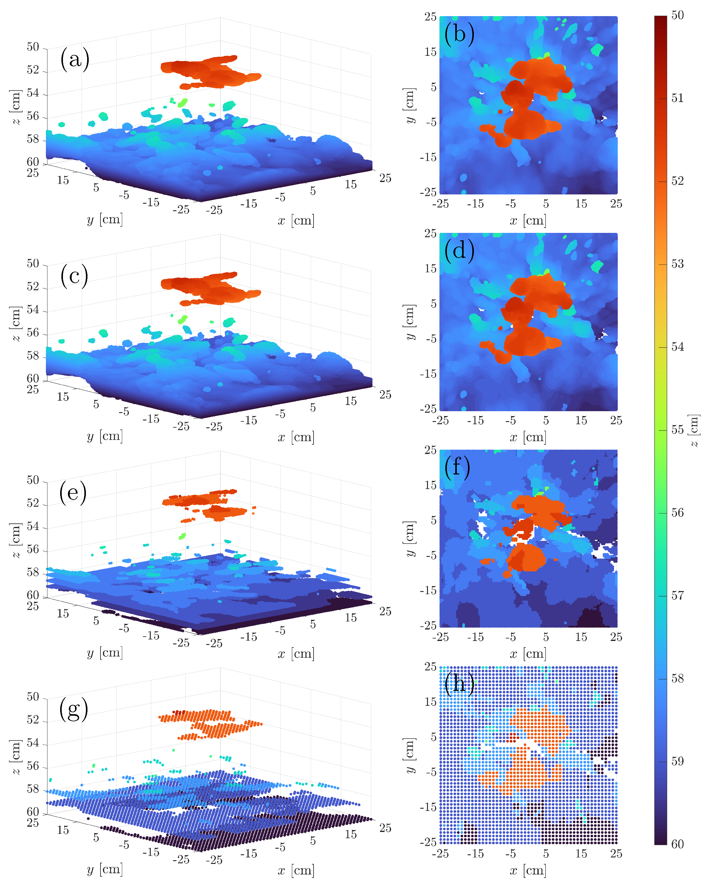
A comparison of the results of 0.05 cm (a,b), 0.1 cm (c,d), 0.5 cm (e,f), and 1 cm (g,h) resolution imaging. The images lose details at resolutions larger than 0.1 cm, but the finer 0.05 cm resolution image provides no further benefit.
Figure 10.
A comparison of the results of 0.05 cm (a,b), 0.1 cm (c,d), 0.5 cm (e,f), and 1 cm (g,h) resolution imaging. The images lose details at resolutions larger than 0.1 cm, but the finer 0.05 cm resolution image provides no further benefit.

Figure 11.
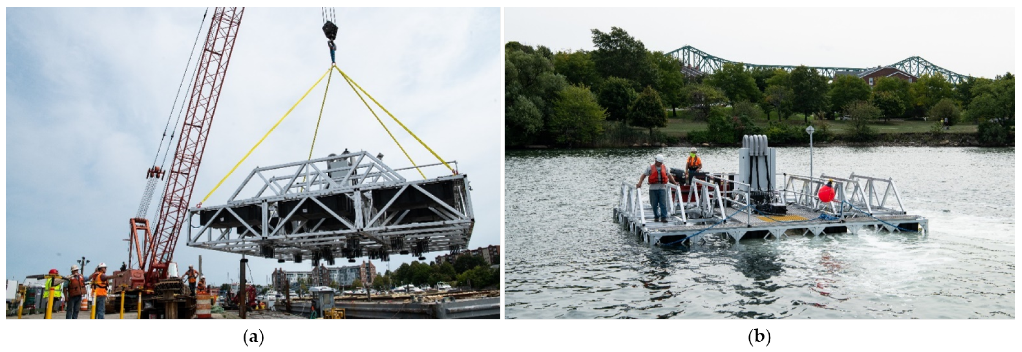
(a) The initial deployment of the oceangoing sparse-aperture sonar. (b) The sonar is towed out to the ocean through the Boston Harbor on 17 September 2020.
Figure 11.
(a) The initial deployment of the oceangoing sparse-aperture sonar. (b) The sonar is towed out to the ocean through the Boston Harbor on 17 September 2020.

Figure 12.
Initial pier-side test results of the oceangoing sparse-aperture sonar. The array layout and range profiles from all transmitter–receiver pairs are shown in (a,b), respectively. The reconstruction point cloud of the pier bottom is shown in (c).
Figure 12.
Initial pier-side test results of the oceangoing sparse-aperture sonar. The array layout and range profiles from all transmitter–receiver pairs are shown in (a,b), respectively. The reconstruction point cloud of the pier bottom is shown in (c).

Figure 13.
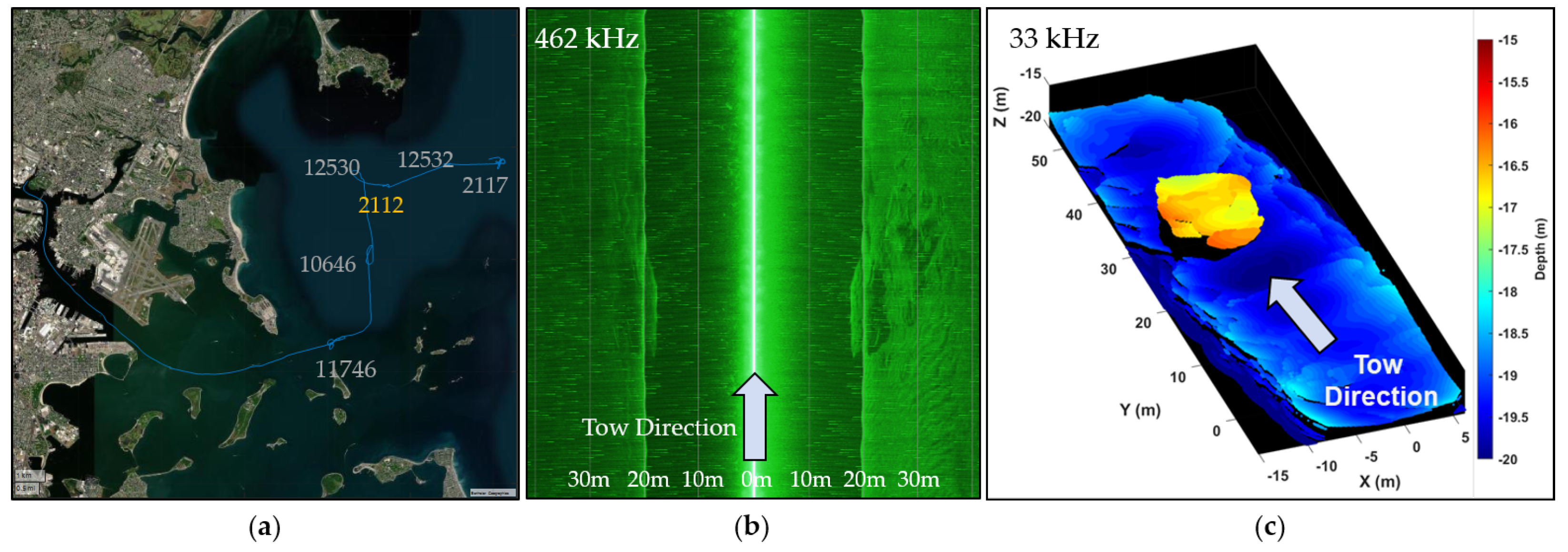
A comparison of seabed imagery of automated wreck and obstruction information system (AWOIS) site 2112, a sunken barge outside Boston Harbor. The site’s geolocation is indicated in (a). (b,c) Show reference imagery from a commercial side-scan sonar and imagery generated with our large sparse array using our initial low-resolution algorithm, respectively.
Figure 13.
A comparison of seabed imagery of automated wreck and obstruction information system (AWOIS) site 2112, a sunken barge outside Boston Harbor. The site’s geolocation is indicated in (a). (b,c) Show reference imagery from a commercial side-scan sonar and imagery generated with our large sparse array using our initial low-resolution algorithm, respectively.

Figure 14.
Power loss with position error simulated based on 33 kHz sonar data.

Figure 15.
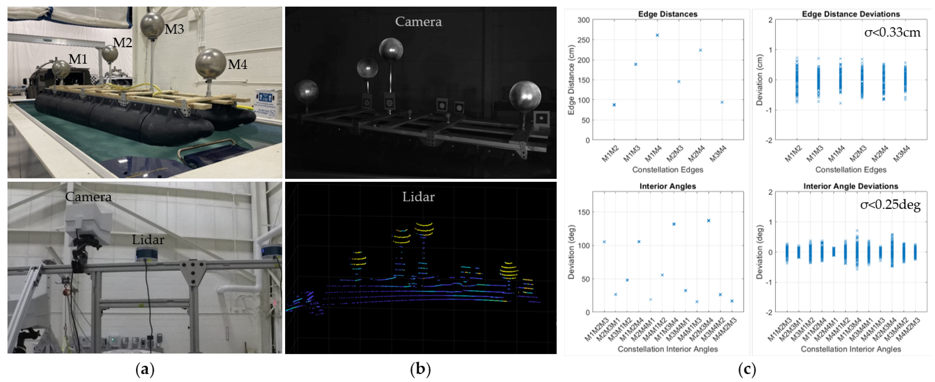
The in-lab test setup for precision-relative navigation is shown in (a). Example data frames from a near-infrared camera and LiDAR are shown in (b). Edge distances and interior angles calculated for tracking the ASV are shown in (c).
Figure 15.
The in-lab test setup for precision-relative navigation is shown in (a). Example data frames from a near-infrared camera and LiDAR are shown in (b). Edge distances and interior angles calculated for tracking the ASV are shown in (c).

Figure 16.
Initial sea testing of custom ASVs and sensors. Precision optical and LiDAR tracking of the vessel from shore (a) and boat (b).
Figure 16.
Initial sea testing of custom ASVs and sensors. Precision optical and LiDAR tracking of the vessel from shore (a) and boat (b).

Figure 17.
The potential cost of an operational sparse-aperture sonar mapping using at least 25 ASVs and our current image reconstruction, focus, and relative navigation techniques.
Figure 17.
The potential cost of an operational sparse-aperture sonar mapping using at least 25 ASVs and our current image reconstruction, focus, and relative navigation techniques.


Table 1.
Signal processing improvements.
| Low Resolution (Existing Algorithm) | Improved Resolution (Future Algorithm) |
|---|---|
| 10 cm voxels | <5 cm voxels |
| Semi-static motion compensation | Full motion compensation |
| Range migration with straight propagation | Range migration with ray tracing |
| Direct blast timing calibration | Autofocus for calibration |
| Measured sound velocity profile | Sound velocity updated during focusing |
| Basic bistatic scattering model | Scattering model optimization |
| Incoherent summing | Coherent processing |
Disclaimer/Publisher’s Note: The statements, opinions and data contained in all publications are solely those of the individual author(s) and contributor(s) and not of MDPI and/or the editor(s). MDPI and/or the editor(s) disclaim responsibility for any injury to people or property resulting from any ideas, methods, instructions or products referred to in the content. |
© 2023 by the authors. Licensee MDPI, Basel, Switzerland. This article is an open access article distributed under the terms and conditions of the Creative Commons Attribution (CC BY) license (https://creativecommons.org/licenses/by/4.0/).
Share and Cite
MDPI and ACS Style
Ryu, P.; Brown, D.; Arsenault, K.; Cho, B.; March, A.; Ali, W.H.; Charous, A.; Lermusiaux, P.F.J. A Wide-Area Deep Ocean Floor Mapping System: Design and Sea Tests. Geomatics 2023, 3, 290-311. https://doi.org/10.3390/geomatics3010016
AMA Style
Ryu P, Brown D, Arsenault K, Cho B, March A, Ali WH, Charous A, Lermusiaux PFJ. A Wide-Area Deep Ocean Floor Mapping System: Design and Sea Tests. Geomatics. 2023; 3(1):290-311. https://doi.org/10.3390/geomatics3010016
Chicago/Turabian StyleRyu, Paul, David Brown, Kevin Arsenault, Byunggu Cho, Andrew March, Wael H. Ali, Aaron Charous, and Pierre F. J. Lermusiaux. 2023. "A Wide-Area Deep Ocean Floor Mapping System: Design and Sea Tests" Geomatics 3, no. 1: 290-311. https://doi.org/10.3390/geomatics3010016