1. Introduction and Overview
Recent increases in Lidar point density have increased the need to filter (or decimate) these large datasets to reduce the memory footprint while retaining acceptable levels of accuracy. Petras, et al. [
1] noted that there are advantages to decimating point clouds in some applications. For example, they pointed out that a Geiger-mode scanner returns 25 pulses per square meter, and this high density increases storage requirements and processing time. The new Curvature Weighted Decimation algorithm, introduced here, is designed to reduce the number of points in a Lidar terrain point cloud dataset while minimizing the elevation accuracy loss of the reduced dataset. The problem we address with Curvature Weighted Decimation (CWD) is a type of data compression algorithm using geometric characteristics of the data to prioritize points for retention or elimination. The goal is to reduce sampled points on a surface while retaining as much positional accuracy of the derived surface as possible. Elevation accuracy is the assessment metric, an important property that impacts other parameters, such as slope and aspect. Though additional values such as curvature or the location and dimensions of linear features (e.g., stream dimensions or watershed boundaries) may be impacted by decimation, the residual accuracy of these metrics is not included in this study.
The number of sampled points is reduced by generating a triangulated surface mesh from the points, then prioritizing points for retention based on each point’s discrete curvature in the mesh. Point retention or elimination is performed in two major steps by first computing dihedral angles between triangle faces and then individual point curvatures based on the mesh. The mesh is generated from the points using the horizontal plane as a 2-tuple independent variable, while elevation is the dependent variable. Due to CWD’s approach, including mesh geometry, the literature reviewed here related to CWD regards not just point cloud reduction but also mesh vertex reduction. CWD is focused on terrain modeling, but the literature review additionally includes the domains of mesh reduction for computer graphics and optimization of small, scanned objects.
1.1. Literature Review
The literature review considers terrain point cloud reduction only after reviewing non-terrain point cloud reduction techniques to set the broader view of the state of the literature.
1.1.1. Non-Terrain Point Cloud Decimation
Most approaches to point reduction entail a step where the points are tessellated into a triangulated mesh so as to reconstitute the surface sampled by the points. The mesh allows an algorithm to conduct more powerful analyses of the points.
Schroeder, et al. [
2] marked vertices in the mesh for removal using a criterion of “distance to plane”. Specifically, if a given point is close enough to the average plane defined by its first-order neighbors, it is selected for removal.
This approach was later named the Quadric Error Metric (QEM) by [
3], which introduced an algorithm for QEM for error metrification. Their approach has become well-established for many subsequent error metrics on non-terrain point clouds. QEM is necessary on non-terrain objects as there is no up-orientation by which to define elevation (or elevation error) as there is for terrain point clouds.
QEM is a way to measure the error introduced by a point removal action at point selection time. The error that would be introduced by removing a point (or in some cases by collapsing a line) is computed as the distance from the point in question to the triangle plane that would remain were the point removed. Points are prioritized for removal when such removal would introduce lesser QEM errors. As mentioned above, this method was introduced by [
3] and was used with modifications by [
4].
Lu, et al. [
5] used QEM, but weighted the QEM error by an approximation of the discrete vertex Gaussian curvature to prioritize edges to collapse.
1.1.2. Terrain-Related Point Cloud Decimation
Mesh-Based Terrain Point Reduction
As Curvature Weighted Decimation uses discrete point curvature to determine which points to retain, the few approaches in terrain modelling which rely on tessellating the terrain points into a mesh are reviewed.
QEM
The volume preservation metric used by [
6] in modelling terrain, is a type of QEM in that by including the areas of the mesh triangles, the offset error cost is a volume. Song, et al. [
7] used Morse Theory to compute QEM via terrain trees to preserve topology (pits, peaks, and saddles) of terrain meshes.
Triangle Line Dihedral Angle
Dihedral Angle between faces uses the angle between planar normals of two adjacent faces (triangle) to prioritize lines for collapse or preservation [
8]. The criterion for line selection for this algorithm is the minimum dihedral angle between faces to be dissolved. Angles closer to 180°, being flatter, are selected for dissolution.
Discrete Gaussian Curvature
Stupariu, et al. [
9] conducted a thorough analysis of various techniques to approximate discrete Gaussian curvature of each point on a mesh applied to terrain applications. They found that the Gauss–Bonnet equation (Equation (1)) performs well for this purpose. Stupariu also observed “Gaussian curvature could be linked to peak/pit/pass-type forms, while the mean curvature seemed to be related to curvilinear shapes such as ridges and channels.” ([
8], p9). This observation is reiterated in the discussion in
Section 4.2.5.
Some researchers have combined some of the above techniques. One example of this [
10], used a combination of QEM with Absolute Curvature to select points for removal in a half-edge collapse technique where one of the two points of a collapsed edge are retained.
Yet this review could find no published literature which applies Gaussian curvature to terrain point cloud decimation. For identifying linear features, the work of [
8], by using dihedral angles of mesh lines, can be used, though they made no mention of this advantage.
Non-mesh-based Terrain Point Reduction
Two primary methods are extant in the literature and in practice for point reduction which does not require triangular mesh generation. The first, sequential decimation, starts at the top of the vertex list in the dataset file and skips a user-determined number of vertexes, n-1, then marks the nth point for retention. GRASS GIS implements sequential decimation in its module
v.decimate [
11]. Moreover, the Point Data Abstraction Library (PDAL) includes a filter which implements sequential decimation [
12].
The second non-mesh-based approach is grid-based. Petras [
13] also provided this type of decimation for GRASS GIS. In the grid option of
v.decimate, points are coalesced by averaging coordinate values of the same grid cell. This technique is a fast operation that bins points into the same grid cells for point preservation determination. Finally, ESRI [
14] provided a Lidar processing tool starting with ArcGIS Pro 2.8,
Thin LAS, which decimates Lidar points using a grid approach.
1.2. Curvature Weighted Decimation and CogoDN
Though theory has been developed to compute Gaussian curvature from triangular surface meshes [
9,
14], and dihedral angle serves similar functionality to mean curvature at certain relative scales, no curvature-based tool to decimate Lidar terrain point clouds has been identified in the present literature review. The approach introduced here, Curvature Weighted Decimation, embodied in the new Free Open Source tool, CogoDN, implements a novel approach to point cloud decimation based on curvature. This is accomplished by first selecting retained points associated with high dihedral angle, then selecting additional retained points stochastically by assigning higher retention probabilities to the ones with higher absolute Gaussian curvature. As is demonstrated in this paper, the result is reduced introduced error after decimation compared with Random Decimation over the range of 15–50%. See
Section 3 and
Section 4.
CogoDN models surfaces using Triangulated Irregular Networks (TINs). CogoDN also models 3D alignments used in roadway and stream restoration design, though the alignment-related functionality is not the focus of this paper. The CogoDN module is free and open source under the Apache 2.0 license. CogoDN is written in C# and runs on NET Core 3.1. It has been tested on Windows 10 and Linux Ubuntu 16.04 LTS. In brief, a user may operate CogoDN by launching the command line application and using commands in interactive mode or by launching it with the name of a command file for batch processing. The executable file performs minimal computation, and the actual computation is carried out in linkable libraries which third-party applications may also link to. Possible future work may entail inclusion of CWD into PDAL as a filter.
A user loads a LAS format (Lidar point cloud format) file into memory using CogoDN, creating a Triangulated Irregular Network model (TIN) from the loaded Lidar points. CogoDN loading of Lidar points has been tested on LAS files downloaded from the North Carolina Department of Public Safety’s (NCDPS) Spatial Data Download page at
https://sdd.nc.gov/ (accessed on 3 December 2022).
CogoDN was used to develop the novel point decimation technique termed Curvature Weighted Decimation (CWD). CWD is compared with Random Decimation as a baseline to assess whether and by how much CWD introduces less error than Random Decimation. The main objective of this paper is to test whether CWD yields more accurate results than Random Decimation and to quantify the difference and the decimation ranges under which differences occur.
1.3. Decimation Generally
Lidar measurement of terrain constitutes signal sampling, where the terrain surface may be considered the signal and the Lidar points are the samples.
Decimation is removing points from the dataset to reduce the data footprint size so that the file can be transmitted and loaded into memory more quickly. Larger terrain patches can then fit into available memory, or models may run more quickly. However, as higher decimations result in lower point counts, details of the terrain, sometimes referred to as microtopography (“critical features” in [
15]), are lost unless there is some way to preserve the points essential to defining the microtopographic features. For some applications, this loss is acceptable, but for other applications, such as flow modeling of small streams, this loss of feature resolution results in inaccurate or even unusable models. This information loss is unfortunate when the original purpose of gathering Lidar at higher pulse densities was to be able to locate such microtopography. Curvature Weighted Decimation seeks to retain higher accuracy of certain types of microtopography while removing the desired percentage of points by eliminating ones with lesser contribution to topographic variability. This reduction in model accuracy is illustrated and articulated in
Section 4.2.8.
1.4. Sequential Decimation
Sequential decimation reduces points by skipping n points and retaining the next point as the data stream is loaded into memory. Sequential decimation has the advantage that omitted points never need to be loaded to the model, thus eliminating the additional processing and memory load required by more elaborate decimation processes.
Three disadvantages of sequential decimation are identified here. First, skipping points without considering the model geometry means important terrain features may frequently be lost. Second, some of the points on the exterior of the Lidar point cloud coverage area are eliminated. This elimination near the boundaries erodes the extent of the TIN hull. Depending on how edge triangles are dissolved or retained, the loss of edge points can make some parts of the Lidar panel inaccessible for measuring elevation. Third, the point-skipping approach of standard decimation limits the permutations of retained points. Specifically, a standard decimation of n points, which would decimate to a percentage of 1/(n+1), can have only n+1 unique variations as determined by the start point of the skipping algorithm. This outcome occurs because sequential decimation does not vary the order of the points as they are being streamed into memory from the file. Yet, thirty distinct runs were required per LAS panel in the present study to measure the effectiveness of CWD to achieve statistical significance. This confidence measure could not be achieved with the low number of permutations available through sequential decimation.
1.5. Random Decimation
Instead of comparing introduced elevation errors between CWD and sequential decimation, we used Random Decimation for the comparison, which was implemented in CogoDN to overcome the second and third disadvantages of sequential decimation. However, the CogoDN Random Decimation implementation misses feature-defining points, as does sequential decimation, which is the desired property as a proxy for sequential decimation. The pseudocode for creating a decimated point cloud by Random Decimation is shown in Listing 1.
| Listing 1. Pseudocode to create a new reduced set of LAS points by Random Decimation. |
FUNC Random Decimate(TIN Surface, percentage).
Step 1. Compute the number of points retained as a percentage of the current TIN Surface point count.
Step 2. Identify and mark hull points for retention.
Step 3. Select additional points to retain until the quota is reached.
Step 4. Tesselate retained points to a new TIN surface.
ENDFUNC. |
Original Tin Surface = Load Tin Surface(source file, classification filter).
Derived Tin Surface = CALL Random Decimate(Original Tin Surface, Decimation Percentage). |
Random Decimation selects Lidar points from the input data in four steps. First, the number of retained points is computed by multiplying the point count by the desired decimation percentage. The desired decimation percentage is the number of points remaining as a percentage of the original point count. Step two is to identify all points on the TIN hull and select those for retention, thus preventing erosion of the TIN hull by points being deselected on it. This step overcomes disadvantage number two of sequential decimation described in
Section 1.4. All remaining points are interior to the TIN model and are candidates for elimination with equal probability. Third, each point is assigned a value of retain probability from the desired target decimation percent accounting for the points already retained on the hull. This approach removes the disadvantage of a limited number of permutations present in sequential decimation. Finally, the retained points are tessellated to form a new in-memory TIN model for subsequent elevation computations.
1.6. Curvature Weighted Decimation
Similar to Random Decimation, CWD eliminates sampled terrain points from a TIN model to represent the same terrain with fewer points and achieve a smaller data footprint. However, CWD seeks a lower introduced elevation error rate for a given decimation percentage than Random Decimation. Listing 2 shows the pseudocode for the top level of CWD processing.
| Listing 2. Pseudocode to create a new reduced set of LAS points by Curvature Weighted Decimation. |
Original Tin Surface = Load Tin Surface(source file, classification filter).
Derived Tin Surface = Decimate CWD(Original Tin Surface, Decimation Percentage, Method Split Percentage (optional, 50% when not specified)). |
CWD achieves reduced introduced elevation error values by selecting points to be retained at locations in the TIN model associated with higher surface curvature. This approach makes points in sharply changing features such as stream banks more likely to be retained than points in areas of low (flat) curvature. The method split percentage sets what percent of retained points are selected by Dihedral Angle Rank Ordering (DARO) and what percent are selected by the Sparsity Weighted Curvature Score (SWCS). These are explained in greater detail in
Section 2. The default value for method split percentage (without overriding) is 50%, meaning half of the points not on the TIN hull are selected first by the DARO algorithm, then the remaining half are selected by SWCS. This strategy permits the study of whether DARO or SWCS improves accuracy more than the other. To assess CWD performance relative to Random Decimation, we compared the elevation accuracy of TIN models decimated using Random Decimation to those decimated with CWD. This process is explained in greater detail in
Section 2.4.
2. Methods
CWD was compared with Random Decimation by running multiple decimations by each method on six panels representing three different terrain types (two each in mountainous, foothill, and coastal lowland topographies of North Carolina) and comparing elevation statistics.
2.1. CogoDN and TIN Hull Dissolving
CogoDN reads points from LAS files following [
16]. After all points are read, it creates a TIN model in memory via Delaunay Tessellation [
17] using MIConvexHull [
18].
Along the TIN hull, some of the triangles of the TIN created by MIConvexHull are not representative of the terrain due to steep slopes or spanned channels. This problem occurs because the tessellation process does not have points from adjacent panels to generate triangles. Without that information, and because it always results in a convex hull tessellation, non-representative triangles are introduced at the edge and must be dissolved from the TIN model before other processing. The dissolving process removes edge triangles only while preserving all point cloud points.
When CogoDN automatically dissolves some exterior triangles, it does so based on certain geometric properties of each exterior triangle immediately after tessellating the points into triangles. CogoDN dissolves exterior triangles by visiting each one to consider it for dissolution. As a triangle is marked for dissolution, its interior neighbor triangles become exterior triangles, which are also considered for removal. This process continues in a breadth-first search until all exterior triangles pass the stop-dissolving criteria. Throughout the dissolution process, if the dissolution of a triangle would disconnect a LAS point from the TIN model, the triangle is not dissolved so as to preserve the point for downstream processing.
The resulting TIN model, now referred to as the main surface, is retained in memory for subsequent operations, including decimation. This retention is especially important in estimating the terrain curvature used by CWD. Further, ground truth elevation values for subsequent elevation error computations are computed from the main surface.
Elevation comparisons are computed at 3 m intervals in both x and y, forming a regular grid. First, grid elevations are computed from the main surface at the coordinates of each grid center. After the main surface elevations are computed, decimation is carried out, either random or CWD, and the introduced elevation error is computed at each grid point as the elevation difference from the main surface. The population of grid elevation errors is then used to compute specific error statistics, which are the basis of the comparison, as specified in
Section 2.4. Efficacy Assessment.
2.2. Random Decimation
CogoDN computes Random Decimation in several steps.
Before computing the decimated points, the module loads all LAS points that pass the selection filter and stores the main surface as an in-memory TIN model;
All exterior points with at least one triangle line on the TIN hull are marked for retention. The remaining points are interior to the TIN hull and are considered available points to be retained or removed;
The target point count is reduced by the number of exterior points already retained, and the new percentage to be retained is computed;
All interior points are assigned this new percentage;
Each point is randomly assigned either true or false for whether it should be retained based on this percentage;
The new, derived TIN surface is created in memory by tessellating the remaining points into triangles.
At this point, other operations may be performed on the derived TIN surface. For this study, elevations are computed for every point on the grid, and introduced elevation error values are assigned to each point by subtracting each derived surface elevation from the main surface elevation of the same grid point. The results of this operation are included in
Section 3.
2.3. Curvature Weighted Decimation
CWD combines two approaches for selecting the points to be retained, especially those in high curvature patches. DARO and SWCS are used in steps 4 and 5a, respectively, to select points for retention.
CogoDN carries out CWD in several steps.
Steps 1–3 and 6 are identical to steps 1–3 and 6 in the Random Decimation process, described in
Section 2.2.
- 4.
All available points are considered for retention using the DARO method by moving some points from the set of available points to the set of points to retain. The retain bit is set to true;
- 5a.
Each remaining point in the available points set is provided a curvature score using the SWCS method. The score is converted to a probability which is weighted by discrete point curvature and point sparsity, termed the sparsity-weighted curvature score;
- 5b.
Points from the available points set are randomly selected to be retained (retain bit is set to true) based on comparison of a random number from a uniform distribution with the sparsity-weighted curvature score.
2.3.1. Underlying Principles
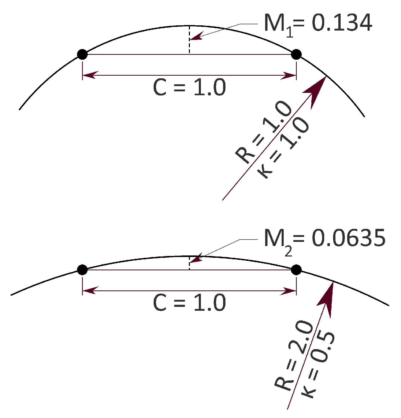
Curvature Weighted Decimation (CWD) is based on the principle that high curvature patches must have a higher density of sampled points to have the same aggregate error values to retain desirable accuracy. This principle is illustrated in
Figure 1 using arc segments of differing curvature.
In
Figure 1, the curvature, κ, of the lower arc segment is 0.5 times that of the upper one. The horizontal separation of the sampled points, C, is the same for each circular arc.
Figure 1 illustrates how the maximum interpolation error between the two sample points, the Middle Ordinate (M), is smaller for M
2 than M
1. This notion may be inverted to understand that where a sampled surface has higher curvature, sampled points must be denser to maintain the same Middle Ordinate introduced error.
Based on this concept, CWD uses Delaunay Tessellation [
17] of the terrain LAS points, also known as a Triangulated Irregular Network (TIN), to model the surface at and between the points. CWD uses properties of the triangles and lines of the TIN to determine the curvature of the TIN model at each interior point. To accomplish the removal of points, those points associated with higher curvature values are more likely to be retained. Conversely, those with lower curvature are less likely to be retained. The desired result is that aggregated introduced error values on the CWD-decimated surface are smaller than on the randomly decimated resulting surface.
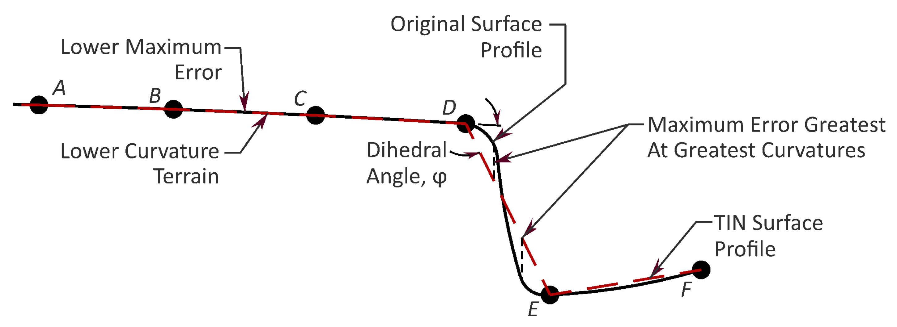
Figure 2 shows a simulated profile cross-section through terrain with a flood plain and a portion of a stream. This conceptual model illustrates how certain terrain features have higher curvature than other types and thus require more points to achieve lower error values.
The decimation process, by definition, entails eliminating sampled points in the derived point set. Using
Figure 2 as an example, removing point B increases the maximum approximation error less than removing either point D or point E. Thus, DARO and SWCS are efficient strategies for identifying points associated with higher curvatures while minimizing the increase in approximation error.
Figure 2 is simplified for illustrative purposes. Specifically, dihedral angles are associated with shared triangle lines, not points in surface meshes embedded in 3D space. Therefore, the dihedral angle is illustrated more accurately in
Section 2.3.3. Importantly, curvature of the triangle surface normals is used, but note that horizontal curvature is not being considered in these methods. For example, a small street with high curvature in its x-y plane alignment would have no additional influence on the selection of points for retention.
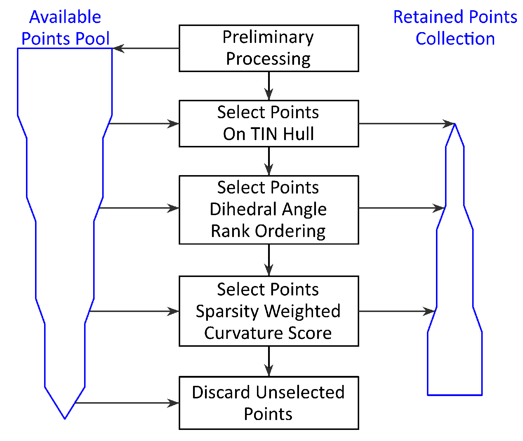
2.3.2. Process Overview
The generalized view of the CWD process is illustrated in
Figure 3. After points are loaded, and the TIN model is created, all original LAS points are in a pool of available points, though none are yet selected to be retained. The processes identify points from the pool of available points and mark them for retention, thus moving them to the collection of used points.
Figure 3 illustrates in broad overview the sequence of processes that select points from the available points pool (or collection), moving those points to the Used Points Collection, which constitutes all points retained after decimation. The width of the blue polygons schematically illustrates the number of points in the collection, showing when and why certain points are transferred from the available points pool to the retained points collection.
Preliminary processing consists of loading the points from the LAS file along with filtering points as specified by the user, then creating the TIN model and dissolving non-terrain triangles at the hull. This TIN model is the one used in downstream processes.
Tin hull point selection, DARO, and SWCS move subsets of available points to the used points collection, which may then be used for other processes. In addition, TIN hull points are selected so that the integrity of the exterior of the LAS panel is not eroded. DARO and SWCS are explained in detail below. This paper does not detail the TIN hull point selection process as it is trivial, while DARO and SWCS are major steps.
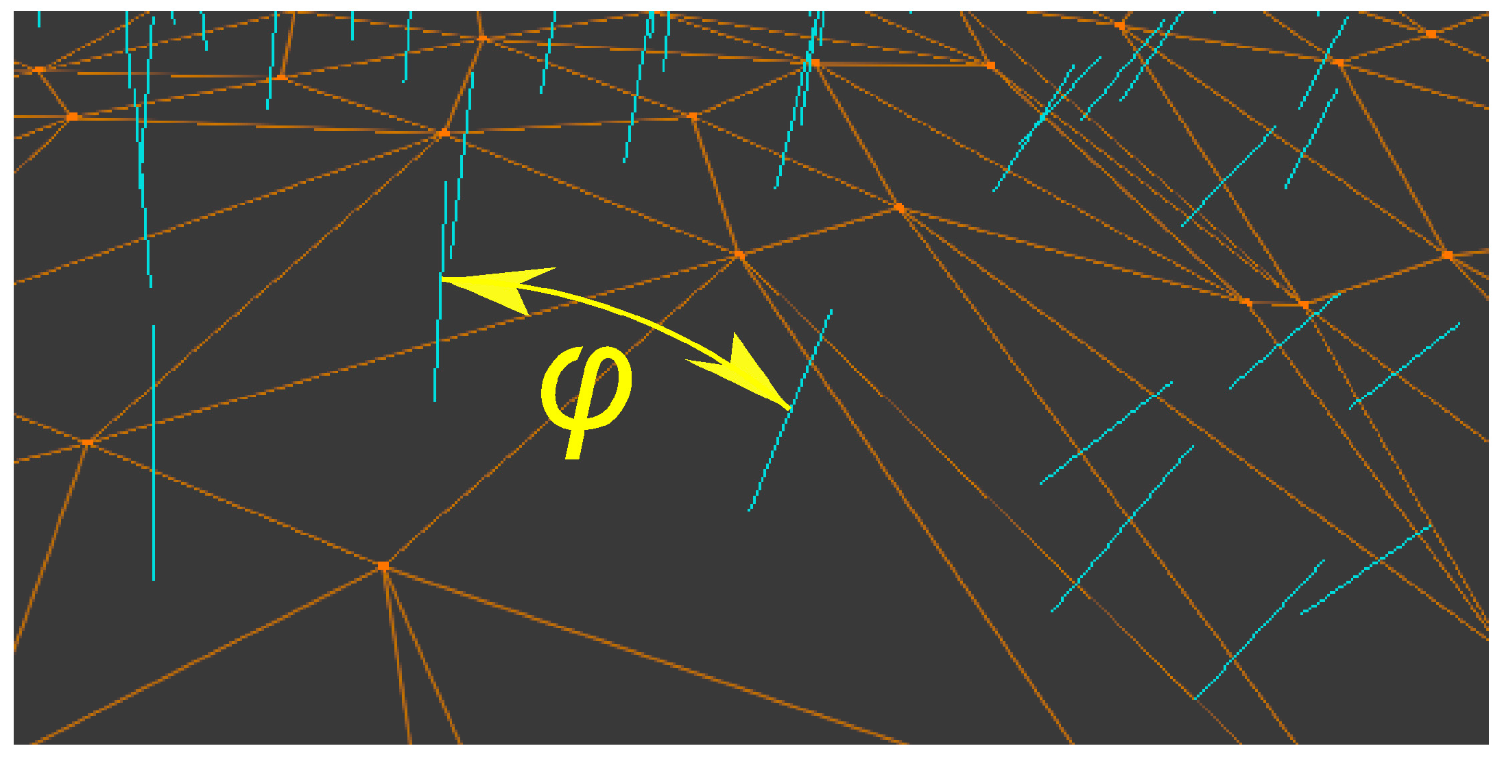
2.3.3. Dihedral Angle Rank Ordering (DARO)
Dihedral Angle Rank Ordering identifies points to be retained based on the dihedral angle of each triangle line. Every interior triangle line connects two triangles. Each triangle has a normal vector that defines the orientation of its plane in space. The dihedral angle of the line is the angle between the normal vectors of the triangles.
Figure 4 illustrates this.
Pseudocode Listing 3 shows the process used to select points for retention using DARO.
| Listing 3. Pseudocode showing steps to select points for retention based on Dihedral Angle Rank Ordering: |
Order the collection of interior triangle lines by decreasing value of the dihedral angle
Set point count to 0
Set target point count to n
For each line in the ordered collection:
If point count > target point count:
Exit For Loop
If line’s left point not already marked for retention:
Mark left point for retention
Increment point count
If line’s right point not already marked for retention:
Mark right point for retention
Increment point count |
CogoDN computes the dihedral angle of each interior triangle line of the TIN model. It then orders the collection of lines by dihedral angle from largest value to smallest. Each line is associated with two Lidar points. The algorithm marks points for retention, starting with the line with the highest dihedral angle and working down the ordered collection until the allotted number of points is reached. Points marked for retention are transferred from the collection of available points to the collection of retained points. The line itself is preserved by retaining the points at the end of a given triangle line, thus the DARO step behaves like an edge preservation algorithm.
This procedure has the effect of retaining points associated with very sharp angles, such as top and bottom of stream banks, retaining walls, or roadway shoulder break points based on the curvature at or near the triangle line.
2.3.4. Sparsity Weighted Curvature Score (SCWS)-Overview
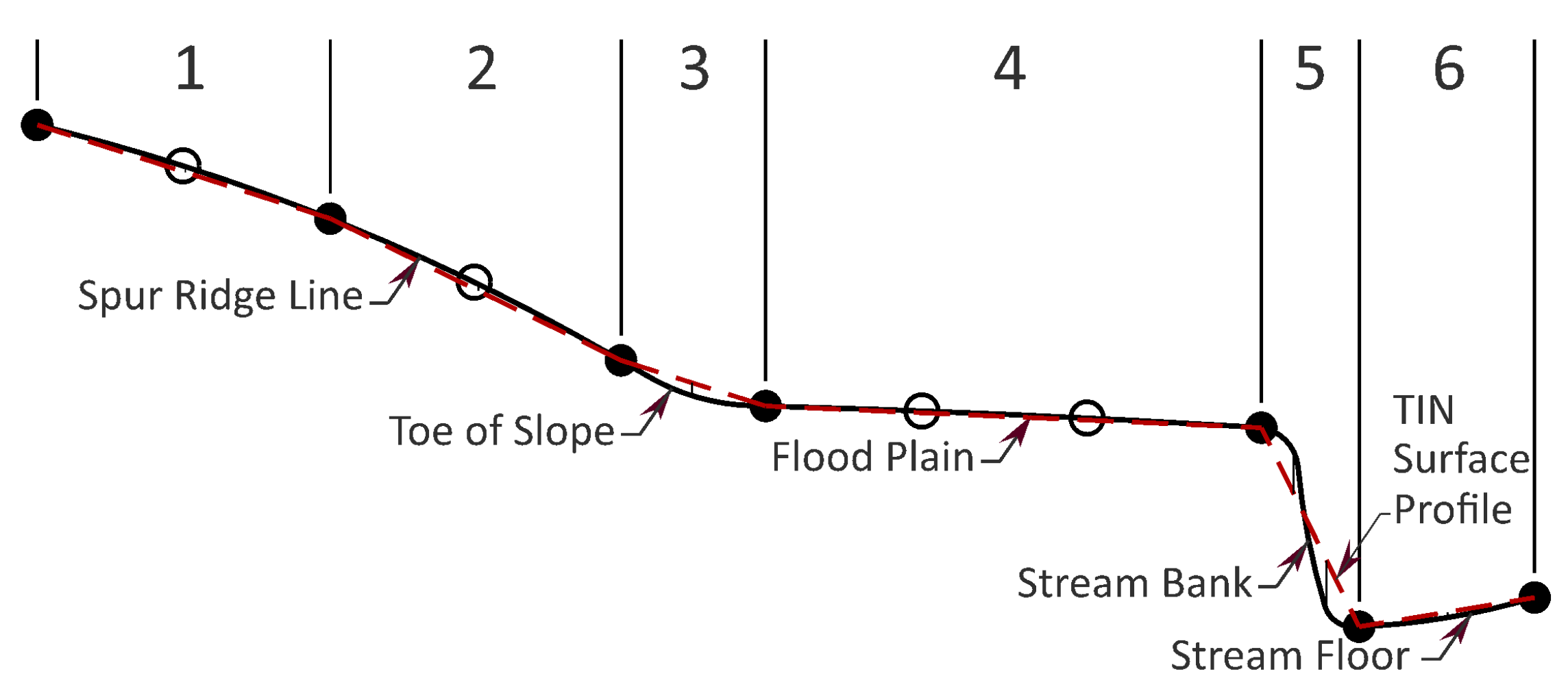
DARO is anticipated to perform well with linear features where the terrain slope breaks so quickly that the feature’s short axis is less than the average sampled point distance. See segment 5 of
Figure 5. However, there is another general case where DARO is expected not to reduce error values effectively. This ineffectiveness in DARO occurs where a larger feature such as a re-entrant or spur has a higher curvature than an open field or flood plain, but lower curvature than the top of a stream bank. This scenario is illustrated in segments 1–3 of
Figure 5. This common case would have greater middle ordinate errors than open fields (segment 4 of
Figure 5) or flat scarps. Therefore, retaining more points on these moderately curved features is desirable to keep average error as low as possible relative to points defining minimally curved sections.
On the other hand, it would be undesirable to eliminate all points from areas of low curvature. Therefore, the SWCS process balances desired outcomes by assigning a curvature “score” to each point remaining in the available points collection. The value is termed a score and not the actual curvature for two reasons. First, each point’s curvature is weighted in significance by its sparsity. A point’s value is an aggregate, not the actual discrete surface curvature at the point. Second, the score is normalized to the range between 0.0 and 1.0, so it can be stochastically compared with a random number generator of uniform distribution over that range. We refer to this value as the retention probability.
In the present context, the sparsity of a point is the reciprocal of the density in the horizontal plane. Ground point density of Lidar datasets is not geometrically uniform, and the SWCS accounts for this to reduce variation in point density in the resulting dataset. Gaps in ground point coverage occur in shadows caused by trees, bridges, buildings, ponds, or other water features. To mitigate this loss of resolution at these locations, the “curvature score” includes not only a fast approximation of each point’s curvature but the contribution of each adjacent triangle is increased if the triangle is large.
SWCS assigns a score to all available points between 0.0 and 1.0 as a retention probability. Higher values are more likely to be retained. The final step in point retention is randomly selecting points from the remaining population based on their probability scores. Because of the computational limitations of a truly random sampling algorithm, we instead transform the distribution of SWCS probabilities such that the mean is near the desired proportion of points to keep (Equation (4)). Thus, the resulting sample contains approximately the desired number of retained points, while requiring only a small number of parallelized passes to perform the selection process.
2.3.5. Sparsity Weighted Curvature Score Details
The Sparsity Weighted Curvature Score is computed using the steps outlined in Listing 4.
| Listing 4. Pseudocode for the Sparsity Weighted Curvature Score point selection algorithm. |
For each point in the available points pool:
Compute the curvature of the point using the Gauss–Bonnet equation (Equation (1)).
Compute the sparsity of each point (Equation (2)).
Compute the raw retain priority score (Equation (3)). |
Normalize the population’s priority score to range from 0.0 to 1.0.
Dilate the normalized scores iteratively to form a probability distribution whose mean is equal to the desired proportion of points to keep. (Equation (4)) |
For each point in the available points pool:
Sample a random number from the range 0.0–1.0 of the Uniform Distribution.
If the point’s retain priority score > the random number:
Mark point for retention. |
The discrete Gaussian curvature, κ, of any given interior point,
P, may be computed using the Gauss–Bonnet theorem [
19], shown in Equation (1).
where F is the collection of all faces (triangles) that contain P, and
is the interior angle of the face at P.
The sparsity of each interior point,
P, is computed as
where
is each face (triangle) in all faces that contain
P, and
is the area of . Equation (2) may be described as assigning one-third of the area of the triangle to each of its three vertices.
The raw retain priority score,
R, of each point is computed by
The sign of Gaussian curvature indicates whether the two principal curvatures curve in the same direction. However, this distinction is unimportant in the current application, which is why the absolute value of the discrete Gaussian curvature is used.
The result of this raw score is that points associated with higher absolute Gaussian curvature are more likely to be selected. Further, the sparsity score, s, is higher for points that belong to larger triangles in the TIN model, so sparse points have a higher retention priority score. Multiplying the two assigns equal weight to each point’s absolute Gaussian curvature and its sparsity. The intention is to make points of higher sparsity, such as those on the edge of a building shadow, more likely to be selected for retention even if the curvature is low.
For the retention priority score to be used in selecting points for retention from the available points collection, the values are normalized to the range 0.0–1.0 by dividing all raw scores by the maximum raw score. At this juncture, the value can be considered the probability of retention, but nearly all points have a very low probability. Because we want to enable a single-pass random selection, we want to transform this collection of retention scores into a probability distribution with mean probability equal to the desired selection rate from the population using a simple Bayes-inspired hyperbolic transformation
T ([
20]).
where
P is the unadjusted probability for each point;
Padj is the adjusted probability for each point;
p1 is the population mean before transformation;
p0 is 1-
p1;
τ1 is the target population mean after transformation;
τ0 is 1–
τ1.
Equation (4) is applied to the retain probability of each point in the population once in a batch, after which the adjusted population mean is recomputed. If the adjusted population mean does not fall within a small tolerance of the desired population mean after a given batch, the values are batch-adjusted again until they are within the tolerance. The mean value converged to tolerance within three parallelized batch runs of Equation (4) during development testing. After an adjusted retain probability value has been assigned to all available points, each point is evaluated for selection based on the algorithm shown in Listing 5.
| Listing 5. Pseudocode showing the process of selecting points using the Sparsity Weighted Curvature Score algorithm. |
Create Random Number Generator (RNG)
For each point in the Available Points Collection:
Random number = obtain new random number over (0.0,1.0] from the RNG
If the point’s retention probability is greater than Random number:
Move point from Available Points Collection to Used Points Collection. |
The random number generator is the standard uniform distribution random number generator for floating point values over the range 0.0–1.0 as provided by the C# programming language. Uniform numbers are required to satisfy the requirement that each point selection is a Bernoulli trial.
2.3.6. Combined Use of the Two Methods
As depicted in
Figure 3, the points associated with sharp dihedral angles are selected first via DARO, leaving SWCS to select from the remainder of the available points collection second. TIN hull point selection and DARO are determinant processes. SWCS is stochastic.
TIN hull point selection moves a small percentage of points from the available points pool to the used points collection. The exact percentage varies across datasets but is generally less than 0.5% of all points in the pool before processing starts. The quota of remaining points to be selected is split evenly by DARO and SWCS. DARO selects points until 50% of the total quota is reached. SWCS selects points up to the remainder of the quota such that the number of selected points equals the original number of points times the desired decimation percentage. Because SWCS is a stochastic process, the exact number of selected points deviates slightly from the indicated quota. No attempt is made to add or trim this excess as it can introduce an unknown selection bias. Though the default split between the DARO and the SWCS quotas is 50/50, assessing how each method contributes to reducing introduced elevation errors is worthwhile. Therefore, tests were conducted in which the DARO/SWCS ratio was set to 20/80 and then reversed to 80/20. This ratio is elsewhere termed the “method split”.
2.4. Efficacy Assessment
The primary question in this research is whether Curvature Weighted Decimation introduces less elevation error than Random Decimation for the same decimation percentage and how to characterize that improvement. In addition, a derivative question is whether and how much the selected method split influences introduced error values.
These questions were assessed by using Lidar .las files from the North Carolina Department of Public Safety’s Lidar repository (
sdd.nc.gov). In this dataset, the four studied panels east of 80° W longitude are QL2. The two studied panels west of 80° W longitude are QL1. The elevation values of each derived TIN model surfaces were compared with the original, pre-decimation TIN on a regular grid with grid points spaced at 3.0 m apart on each axis covering the entire LAS panel area. For the panels of dimension 1524 × 1524 m, this results in a grid of 2,322,576 sampled elevation differences. For the panels of 762 × 762 m, there are 580,064 grid points.
It must be emphasized here that the research deals primarily with points in point clouds and the TIN models tessellated from them. The grid used for the efficacy assessment is a temporary, in-memory only grid. It is neither a data source nor a data product.
Six panels were selected from the North Carolina Lidar dataset and are detailed below. The same suite of runs was made on each of the six panels.
Table 1 shows a summary of these runs.
Each type–split–percentage combination was run thirty times to achieve statistical significance, collecting specific statistics on introduced elevation error values, as shown in
Table 2. The total number of runs was 7200.
Point count is not shown on any chart, though the values are available in the
Supplemental Information. Results are visualized in charts for the following combinations of decimation type (
Table 3). Only charts for root mean square error are provided herein. The other charts are available under
Supplemental Information.
Root mean square error was computed using Equation (5).
where
Δz is the elevation difference between the undecimated TIN surface and the derived TIN surface, and
N is the total number of points in the grid.
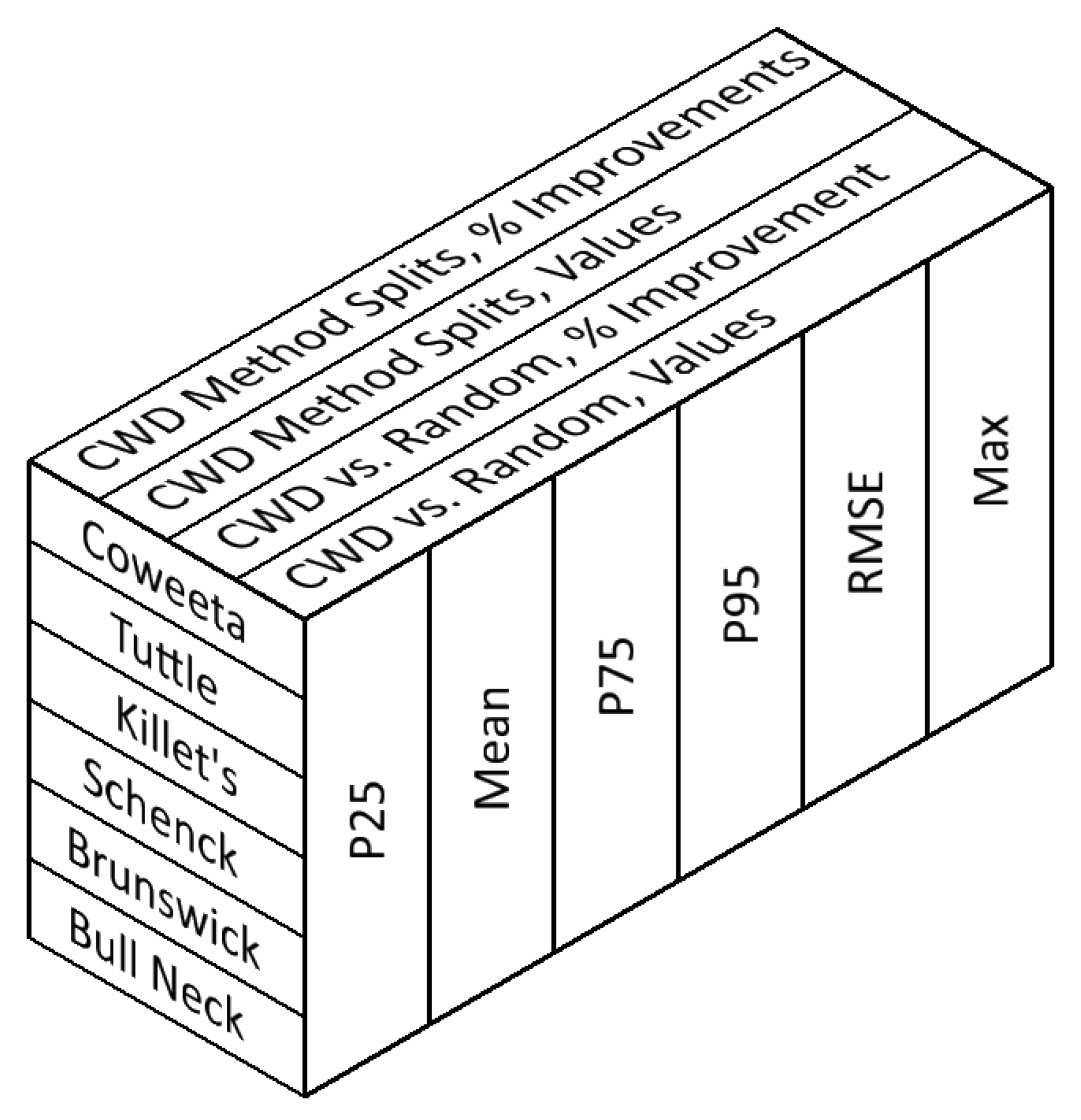
The full chart combinations may be visualized in a 3D matrix cube, as shown in
Figure 6, yielding a total of 144 charts.
Data (Study Panels)
At publication time, CogoDN had only been tested to read LAS files that have been downloaded from North Carolina’s Lidar repository at sdd.nc.gov. Future development and testing are intended to enable the reading of LAS files from other sources as well as LAZ files.
The study focused on 6 LAS panels available from sdd.nc.gov. The six panels were chosen to be from a variety of terrain forms, and for the most part, on public lands to allow site visits. The six panels are characterized in
Table 4. Panel names are assigned only for the scope of the present paper.
The Coweeta and Tuttle panels are QL1 data quality. The other four panels are QL2 data quality, as reflected in the second column of
Table 4.
The North Carolina Department of Public Safety maintains the Lidar repository at sdd.nc.gov. Individual LAS files, also called panels, are named as unique integer identifiers. Panels are accessible from the site via the unique identifier.
Table 5 shows the unique identifier for each of the six panels and the total point count of ground points (Category 2) and road surface points (Category 13). North Carolina’s use of Category 13 for road surface in this dataset is an exception to the ASPRS standard [
16,
21].
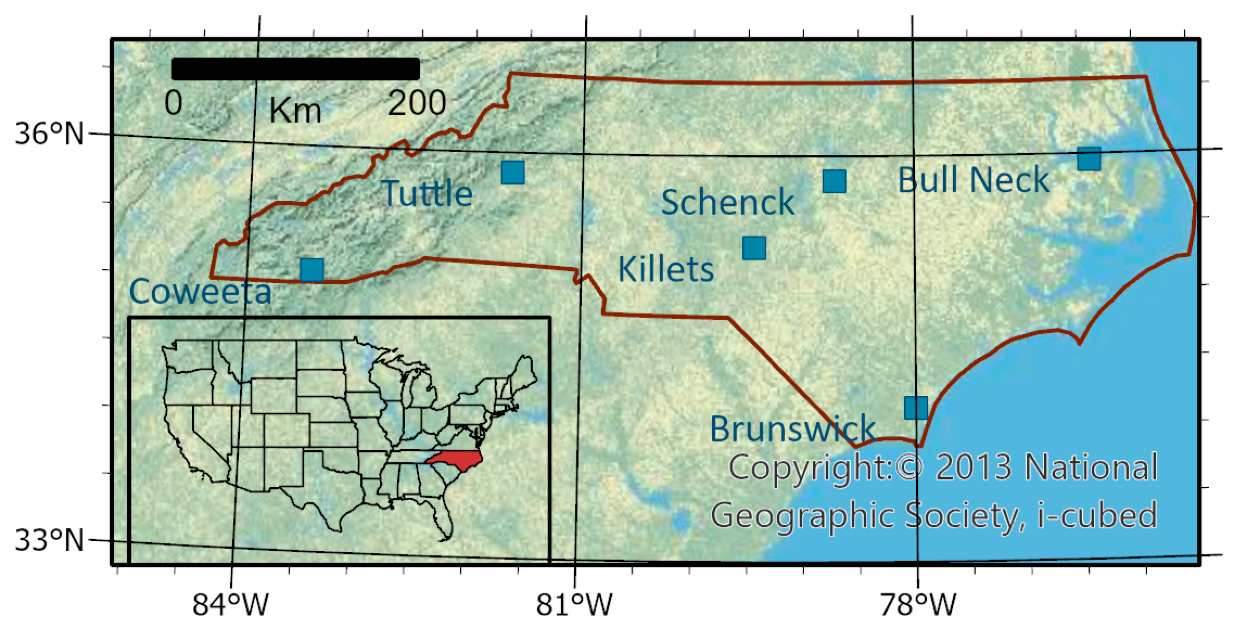
The geographical location of the six panels is shown in
Figure 7.
3. Results
Figure 8 and
Figure 9 provide details and examples of the TIN models of the Lidar dataset for the Tuttle dataset at Celia Creek in Gamewell, NC.
3.1. Random Decimation versus CWD
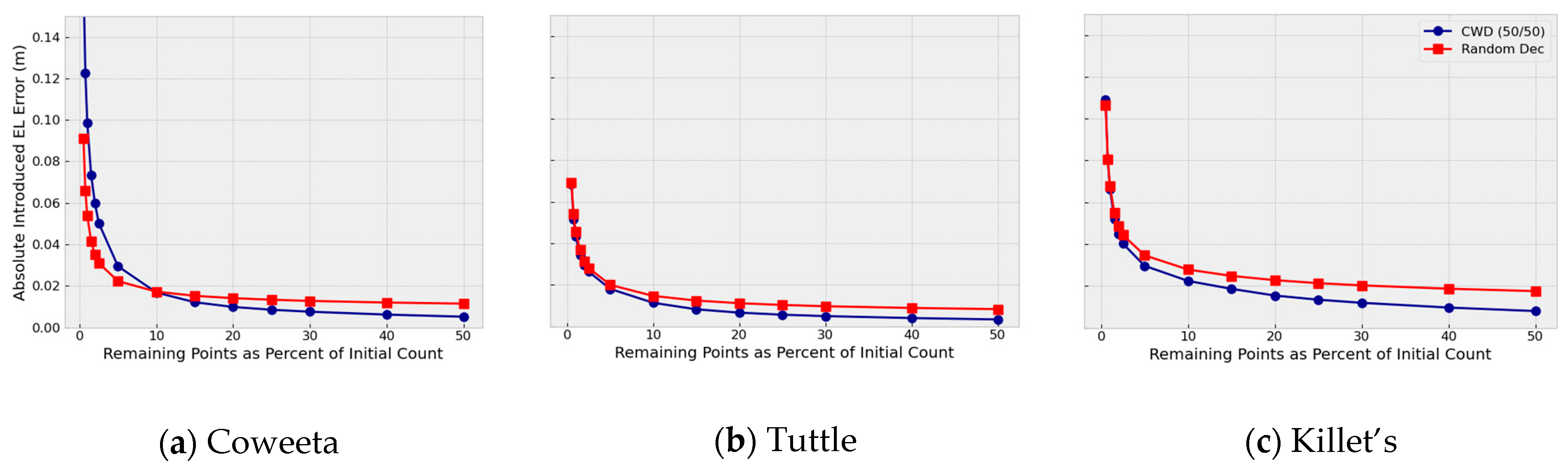
Figure 10 shows the root mean square elevation error statistic results when comparing Random Decimation to curvature weighted decimation for all six study areas. The other statistics, Absolute Error, P25, Mean, P75, P95, and Maximum, are available in the
Supplementary Data section.
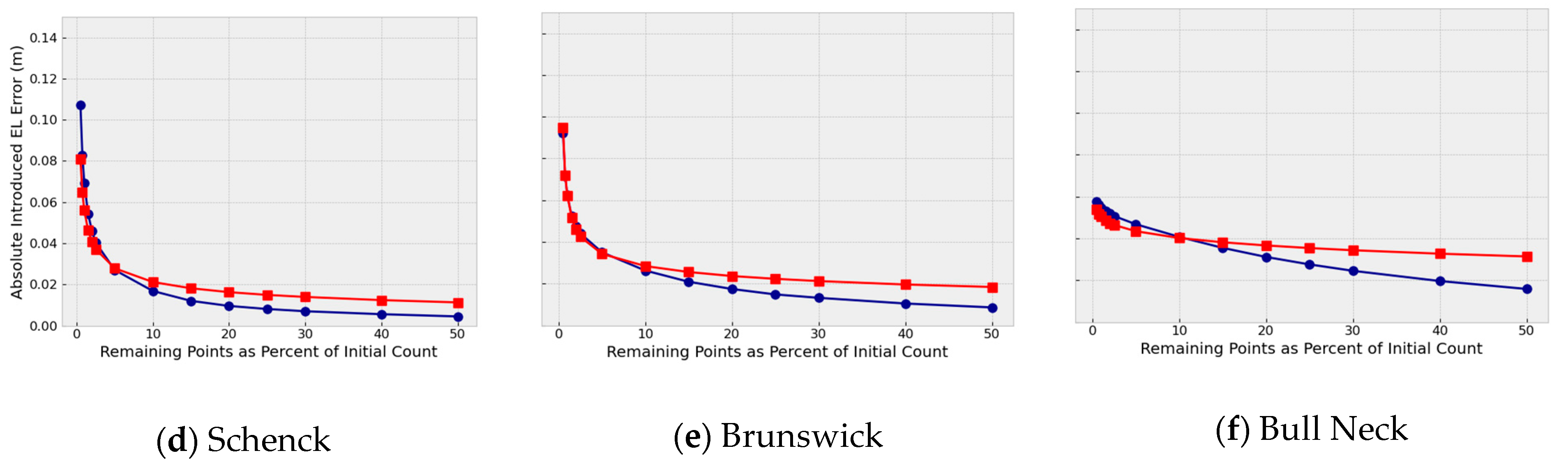
Figure 11 shows results by what percent CWD improves the introduced error for all panels for the root mean square statistic.
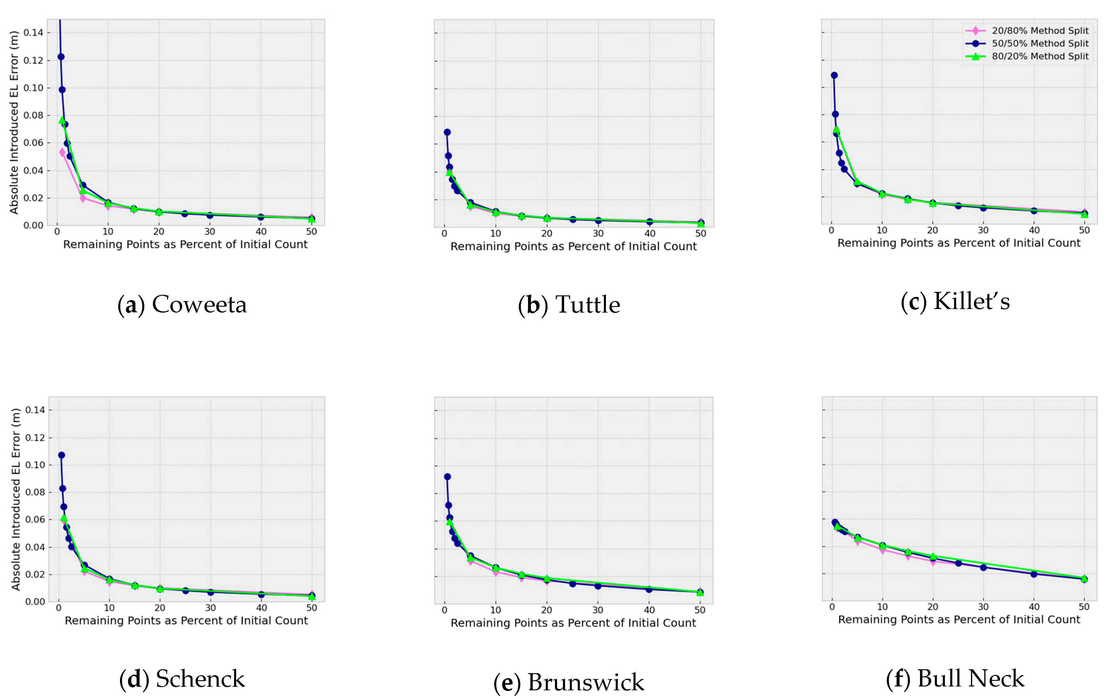
3.2. CWD Varying Method Split
CWD uses two major steps, DARO and SWCS, to select Lidar points for retention. In order to determine whether one of those methods reduces introduced error better than another, runs were made in which the number of points selected by each method was varied. One set of runs was carried out with 80%-DARO and 20%-SWCS. The other set of runs used 20%-DARO and 80%-SWCS.
Figure 12 shows Absolute Introduced Error for method splits of 20% DARO /80% SWCS, 50/50%, and 80/20%.
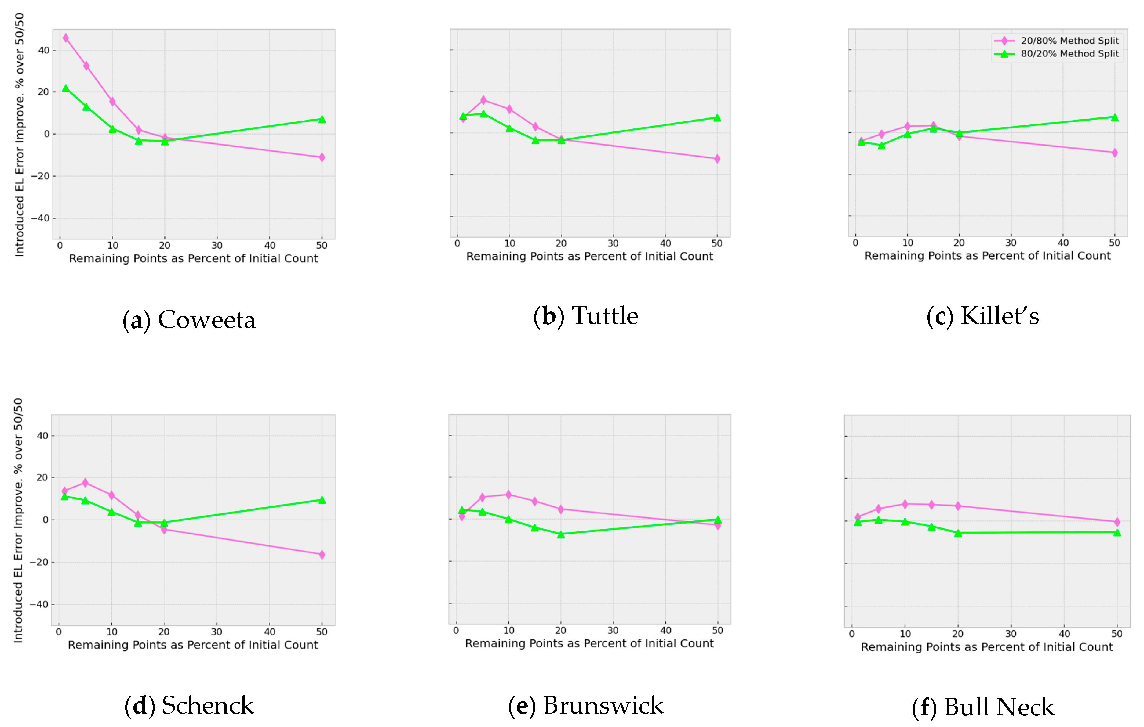
Figure 13 shows Absolute Introduced Error for 20/80% and 80/20% as a percentage of 50%-DARO and 50%-SWCS (50/50), which is the default setting.
4. Discussion
Curvature Weighted Decimation reduces introduced error statistics on all study panels over all statistical metrics computed in this study. The improvement range generally persists from 15% of initial point count and upward. Improvements vary by statistical type, though improvements in the P25 Introduced Error (IE) and Maximum IE are compelling. Other statistical metrics, though not as pronounced as P25 and Maximum, are noteworthy.
Unexpectedly, for all panels and among all statistical metrics, at decimation percentages less than 10%, CWD lost its advantage over Random Decimation (RD), with CWD performing worse than RD. We interpret this as the threshold for defining the terrain being crossed at approximately 10%.
The Introduced RMS Elevation Error Improvement ratio charts (
Figure 11) show for each decimation rate what percent CWD improves over Random Decimation. These results are useful to understand how much better CWD performs over Random Decimation from 15% and upward. Further, they show how much worse CWD performs compared with Random Decimation below the 10% decimation threshold.
Another way to assess the improvement of CWD over RD is to consider the introduced error value of Random Decimation at 50% and determine which CWD rate achieves the same introduced error. This approach is summarized in
Table 6.
Thus, for the same RMS error introduced by 50% Random Decimation, CWD can decimate the point dataset at approximately 16.6% to achieve around 200% increase in land area covered for the same number of points; therefore, on balance, CWD may be recommended for Lidar point decimation at the rate of 15% and higher.
4.1. Analysis of Method Split
Curvature Weighted Decimation uses two major steps to select points for retention. Points are first selected for retention based on a rank ordering of all internal triangle line dihedral angles. Then, lines with higher dihedral angles are preserved by marking each line’s end points for retention. In the second step, additional points are selected based on the absolute value of the discrete absolute Gaussian curvature with an additional factor to favor points with a higher sparsity.
The question presents itself as to which of these two methods is better at selecting points more representative of the terrain. Method split, the ability to shift the percentage of points selected in DARO and SWCS was introduced to understand this question. Point percentage selection was used to generate the datasets displayed in
Figure 13. Runs in which method split is set to 20/80% allow 20% of the retained points to be determined by DARO. SWCS selects the remaining 80% of the retained points. The second set of runs was made in which these proportions were swapped.
For non-coastal-plain lidar site panels (e.g., excluding Brunswick and Bull’s Neck), at 50% decimation, 20/80% shows improved performance over 50/50% and 80/20%, which means SWCS (based on Gaussian curvature) works better in these cases. The improvement is on the order of 10%. This improvement is not present for the two coastal plain panels. The lack of improvement for the coastal plain panels may be due to the reduced variability there, or the reduced Lidar point density of the eastern NC panels.
Below 20% decimation, however, there is no clear advantage. Because of this, the default method split in CWD remains at 50%, though the command option to alter method split continues to be available at the CogoDN command line if practitioners wish to investigate how to minimize introduced error results.
4.2. Caveats and Weaknesses of CWD
4.2.1. Break Points on Sharp Slope Breaks
The source data are points only. Thus, nothing in the LAS dataset indicates how to tesselate the points, such as break line featurization. The tessellation is accomplished in CogoDN by MIConvexHull [
18] using only the x and y coordinates. Elevation values of the points are present for downstream computations. This approach allows triangle lines to cross sharp break points such as stream bank tops or shoulder slope breaks without forcing a line to be parallel to the break line of the terrain. This approach means that some lines, though correct for the Delaunay Tessellation, are not the best fit to the terrain. This drawback should be noted when using this or any other unmodified Delaunay Tessellation approach.
Though the insertion of break lines at features would remedy this shortcoming, such work is labor intensive. Our goal is to provide a tool which does not require intensive human data entry such as introduction of break lines. Automated estimation and insertion of break line locations is a potential area of future research for terrain point clouds.
4.2.2. Local Extreme Points
CWD does not attempt to preserve local extreme points. This omission may not be important for high points, but some drainage studies, especially at the entrance and exit to pipe culverts, may benefit from modifying the decimation algorithm so as to preserve local minima in certain cases. This does not mean all local extrema are removed from the dataset. It means that local extrema with low curvature and low sparsity are more likely to be removed from the dataset. Low points at or near culverts often have high curvature and therefore be retained anyway.
4.2.3. Unrepeatable Point Preservation
The step of implementing SWCS is stochastic. Therefore, two runs over the same dataset at the same decimation percentage do not select all the same points during the SWCS process. Nonetheless, points with higher Sparsity-Weighted Curvature Score values are always more likely to be retained than points with lower values. Point selection at this step is conducted concurrently on all available processors, so no simple resolution of this item is anticipated to be developed.
4.2.4. Noise
Measurement noise is present in all three coordinate dimensions for every point. No effort is made in CWD to identify or remove noise. This study treated the dataset as if noise is low enough so as not to matter. However, in some datasets, especially ones with large areas of low curvature over a rough surface, such as a tilled field, the noise may become a significant factor in altering the discrete curvature of each point as compared with the actual curvature of the sampled surface. CWD provides clear improvements over Random Decimation despite this concern.
4.2.5. Curvature Types and Dihedral Angle
DARO uses the rank ordering of dihedral angles to preserve points existing along sharp terrain breaks. An alternate way to accomplish this would be to use Absolute Curvature [
9,
20]. Possible future work on CWD as it is embodied in CogoDN is to use Absolute Curvature in place of DARO. The following expands on why this would be advantageous.
Curvature of a 2D surface in three dimensions has two components. These are termed Principal Curvatures. κ1 is the curvature on axis tangent to the surface which has the highest curvature in absolute value. κ2 is also tangent to the surface and always perpendicular to κ1. κ2 is the curvature on axis tangent to the surface which has the lowest curvature in absolute value.
The are several approaches to aggregating the two curvatures into a single value for the point of interest on the surface.
Table 7 explains these various types of curvature measurement.
It is important to note that the Gaussian curvature of some curved surfaces is zero (e.g., on a cylindrical fillet) because κ2 of a cylinder is 0, and Gaussian curvature is determined by multiplication. For example, this may happen in terrain at break lines such as retaining walls, stream banks (top or bottom), or roadway shoulders. Thus, points on or near the break line would not be prioritized highly by Gaussian curvature, which is the basis of the SWCS step. Therefore, this reality is why the DARO step was introduced. By determining the dihedral angle of every shared triangle line, such break points are located and marked for retention, as depicted in
Figure 3. DARO improves the probability that CWD preserves the top of the stream bank, for example, as illustrated in
Figure 9.
Nevertheless, DARO has the weakness that if a break line fillet has a horizontal width greater than the point sample distance, the cylindrical fillet can be overlooked by falling across multiple triangle lines. Mean curvature is not well suited for addressing the problem as it also may be close to zero for saddle patches (when κ2 approaches -κ1). Therefore, a metric based on Absolute Curvature may improve results over dihedral angle rank order for this limited case. Possible future work can include investigating whether replacing the DARO step with a similar step based on Absolute Curvature reduces introduced error values. The modification to carry out such research would include using the Discrete Absolute Curvature equation [
23].
4.2.6. Boundary Points
CWD retains all points on the boundary of the TIN hull in the initial step after loading. CWD identifies points close to the panel boundary; every point is automatically selected for retention. A small number of additional points can be allocated to DARO and SWCS for retention if a method were developed to mark some points for removal from among the boundary points. This removal may improve the landform’s overall representation, particularly at the lower percentage retained values.
One approach to decimating boundary points would be to adapt the Ramer–Douglas–Peucker line simplification algorithm [
24] for 3D space strings and apply this to the 3D space string of the TIN hull. Alternatively, point reduction can be carried out by a deflection and distance approach to each point to identify and mark for retention points with higher deflection values and higher adjoining line distances. This tactic can be considered Sparsity Weighted Curvature Scoring for a one-dimensional subspace embedded in a volume. Either of these is a good option if adjacent Lidar panels are unavailable. However, a line simplification algorithm may not be the best if the curvature of the points is not known. For the curvature of the boundary points to be known, points from adjacent panels need to be loaded and included in the intermediate Delaunay Tessellation. Such an approach can be developed for possible future research.
4.2.7. Loss of Roadway Points
It is anticipated that points defining the paved roadway surface are being decimated at a high rate relative to other kinds of terrain due to roadway designers seeking to reduce areas of high curvature. Because of this, points that can be used to find edge of pavement or crown location are decimated more heavily than the decimation percent specified by user input. This effect is desirable for open fields or parking lots, but if the end use of the Lidar dataset is to include roadway surface analysis, the decimation rate should be adjusted upward at the user’s discretion. Possible future development can include an approach that identifies roadway points from the point classification and preserves edge-defining points and cross-slope defining points while eliminating points interior to the roadway.
4.2.8. Derived DEM Products
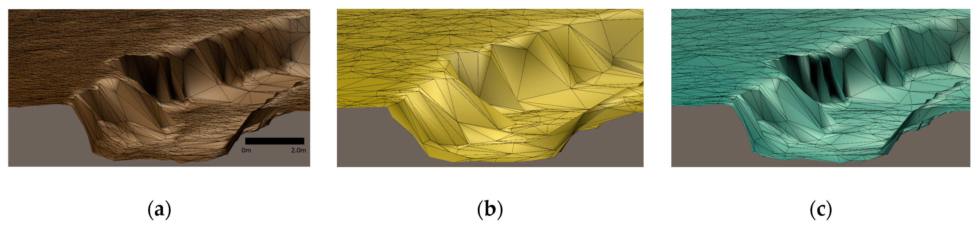
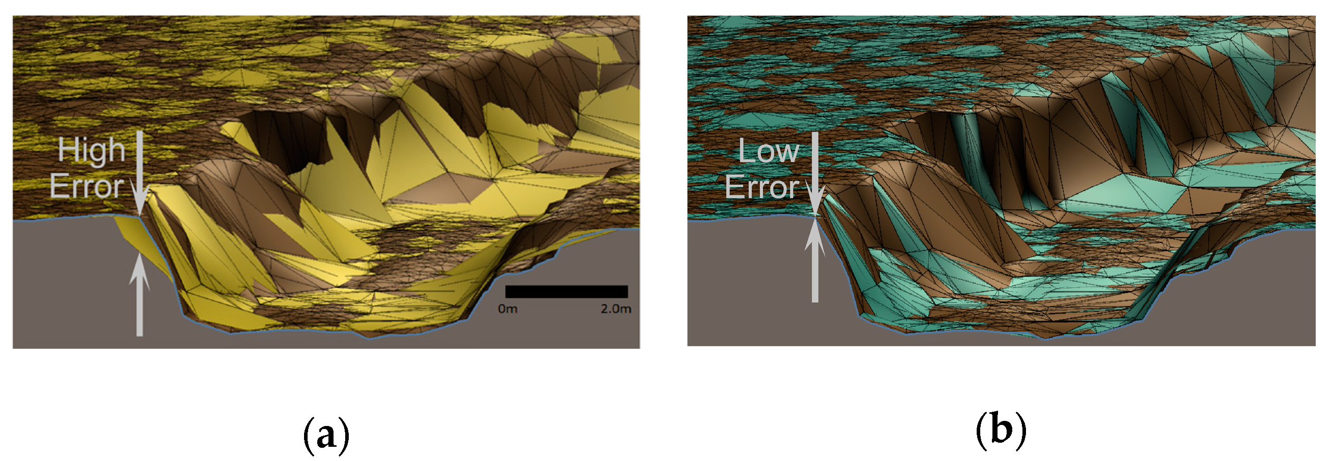
If a raster Digital Elevation Model is derived from a randomly decimated point cloud or a Curvature Weighted Decimated point cloud, it is anticipated that the CWD-derived DEM is more accurate over the decimation range of 15–50%. This is because random and sequential decimation, by disregarding the discrete curvature of the LAS points, tends to strike chords which undercut or overshoot decimated points in the intermediate in-memory TIN. This undercutting is illustrated in
Figure 9a at the stream bank location marked “High Error”.
In
Figure 9a,b, the front clipping plane of the image causes the triangulated mesh to show an example of a cross-sectional profile for the stream. This illustrates why CWD tends to introduce less elevation error totals than random or sequential decimation. The text labels “High Error” for
Figure 9a and “Low Error” for
Figure 9b show examples of this. The generation process from a randomly decimated terrain surface point cloud would carry this error forward into the DEM data derived from it.
The cross-section clipping plane of
Figure 9a,b also underscores the loss of accuracy around the microtopography of streams. Were one of these cross sections included in flood modelling software, the hydraulic geometry of the CWD-decimated dataset (image b) is more accurate than that for the randomly decimated dataset (image a). This effect would also be present for other types of microtopography such as roadway break lines and retaining walls. This illustrates the claim in
Section 1.3 (decimation generally) that random or sequential decimation may result in inaccurate or even unusable models, in this case, for hydraulic modelling of bank full flow or higher.
Future research can investigate the veracity of this anticipated improvement. For example, the study carried out by [
15] decimated the raw Lidar points via sequential decimation. This study can be repeated using Curvature Weighted Decimation as the decimation algorithm to determine whether and by how much this alters the final results. Similar positive impacts may be found if CWD were used in the study carried out by [
25].
Future research can investigate the veracity of this anticipated result. For example, the study carried out by [
15] decimated the raw Lidar points via sequential decimation. This study can be repeated using Curvature Weighted Decimation to determine whether and by how much the change in decimation algorithm alters the final results.
4.2.9. Other Data Sources
Though the focus of this paper is the decimation of Lidar terrain point clouds, the information available from the temporary in-memory TIN model of the undecimated point cloud is anticipated to be of value in point clouds from photogrammetric inputs. Specifically, the information available from the in-memory TIN model consists of point sparsity, dihedral angle between faces, and discrete Gaussian curvature.
Further, these parameters may be used to develop new routines for classifying unclassified datasets. This topic can be undertaken as future research.
5. Conclusions
This paper introduces and assesses for effectiveness Curvature Weighted Decimation, a new point decimation algorithm based on dihedral angle of TIN triangle lines and discrete Gaussian curvature of other points of the dataset. In addition, because Lidar sampling of terrain may have varying point sparsity, the algorithm includes an adjustment to homogenize sparsity. CWD is demonstrated to have lower introduced error for the resulting terrain mesh than Random Decimation over the decimation range of 15–50%.
This paper also introduces CogoDN as a new free, open-source software (FOSS) module that runs on multiple platforms, which we use to develop Curvature Weighted Decimation. CogoDN allows practitioners to use its various features, but also modify or extend them.
In addition to the ones noted in the Discussion (
Section 4. Discussion), other possible future developments which will increase the utility of CogoDN for terrain analysis and processing include the ability to cut profiles and cross-sections at the intersections of Horizontal Alignments for roadway, railway, and stream restoration work, and real-time visualization of the points and the mesh using a 3D viewer such as Unity3d, Blender, or Unreal Engine.
As Lidar point sampling of terrain becomes more common and technological advances boost sampling rates, the need to reduce redundant points for efficient modeling, visualization, and analysis continues to increase. Curvature Weighted Decimation, embodied in CogoDN, is available to practitioners for this kind of work. In addition, since it is FOSS, other researchers can use the implementation of CogoDN presented here or clone the project and make their own modifications public. Finally, as is the benefit of all FOSS packages over proprietary systems, making all source codes available to the public means that the researcher can extend CogoDN with their ideas of core level algorithm concepts or modify the algorithm to suit a particular application. This may be significant as the code to implement many commonly used TIN models is generally unavailable to the practicing GIS and Lidar processing communities.
Author Contributions
Conceptualization, P.T.S.J.; Methodology, P.T.S.J. and C.D.J.; Software, P.T.S.J.; Validation, P.T.S.J. and C.D.J.; Formal analysis, P.T.S.J.; Investigation, P.T.S.J.; Resources, P.T.S.J.; Data Curation, P.T.S.J.; Writing—Original Draft Preparation, P.T.S.J. and C.D.J.; Writing—Review And Editing, L.G.T., K.W.W., G.B.B. and S.A.C.N.; Visualization, P.T.S.J.; Supervision, S.A.C.N.; Project Administration, P.T.S.J.; All authors have read and agreed to the published version of the manuscript.
Funding
This research received no external funding.
Data Availability Statement
Original Lidar LAS files are available from the North Carolina Department of Public Safety’s Spatial Data Download website (sdd.nc.gov). The files are also included in the
Supplementary Material section of this paper. All data are placed in the public domain by the state of North Carolina.
Acknowledgments
The authors wish to thank Anna Petrasova and Vaclav Petras for their advice on Lidar noise. We also thank Luke Schiltz for his coding contribution to CogoDN to generate raster data layers from the sample grid.
Conflicts of Interest
The authors declare that there is no conflict of interest.
References
- Petras, V.; Petrasova, A.; McCarter, J.B.; Mitasova, H.; Meentemeyer, R.K. Point Density Variations in Airborne Lidar Point Clouds. Sensors 2023, 23, 1593. [Google Scholar] [CrossRef] [PubMed]
- Schroeder, W.J.; Zarge, J.A.; Lorensen, W.E. Decimation of triangle meshes. In Proceedings of the 19th Annual Conference on Computer Graphics and Interactive Techniques, Chicago, IL, USA, 26–31 July 1992; pp. 65–70. [Google Scholar]
- Garland, M.; Heckbert, P.S. Surface simplification using quadric error metrics. In Proceedings of the 24th Annual Conference on Computer Graphics and Interactive Techniques, Los Angeles, CA, USA, 3–8 August 1997; pp. 209–216. [Google Scholar]
- Ghazanfarpour, A.; Mellado, N.; Himeur, C.E.; Barthe, L.; Jessel, J.-P. Proximity-aware multiple meshes decimation using quadric error metric. Graph. Model. 2020, 109, 101062. [Google Scholar] [CrossRef]
- Lu, S.; Yang, H.; Han, C.; Zhang, T.; Zhang, Y. Simplification Algorithm of half-edge collapse 3D Model Based on Weighted Curvature. In Proceedings of the 2021 International Conference on Electronic Information Engineering and Computer Science (EIECS), Changchun, China, 23–26 September 2021; pp. 272–277. [Google Scholar] [CrossRef]
- Guinard, S. Simplicial Complexes Reconstruction and Generalisation of 3d Lidar Data in Urban Scenes. Ph.D. Thesis, Université Paris Est-Marne-la-Vallée, Paris, France, 2020. [Google Scholar]
- Song, Y.; Fellegara, R.; Iuricich, F.; De Floriani, L. Efficient topology-aware simplification of large triangulated terrains. In Proceedings of the 29th International Conference on Advances in Geographic Information Systems, Beijing, China, 2–5 November 2021; pp. 576–587. [Google Scholar] [CrossRef]
- Oryspayev, D.; Sugumaran, R.; DeGroote, J.; Gray, P. LiDAR data reduction using vertex decimation and processing with GPGPU and multicore CPU technology. Comput. Geosci. 2012, 43, 118–125. [Google Scholar] [CrossRef]
- Stupariu, M.-S. Discrete curvatures of triangle meshes: From approximation of smooth surfaces to digital terrain data. Comput. Geosci. 2021, 153, 104789. [Google Scholar] [CrossRef]
- Li, L.; He, M.; Wang, P. Mesh simplification algorithm based on absolute curvature-weighted quadric error metrics. In Proceedings of the 2010 5th IEEE Conference on Industrial Electronics and Applications, Taichung, Taiwan, 15–17 June 2010; pp. 399–403. [Google Scholar] [CrossRef]
- Petras, V.; Petrasova, A.; Jeziorska, J.; Mitasova, H. Processing UAV and LIDAR point clouds in grass gis. Int. Arch. Photogramm. Remote. Sens. Spat. Inf. Sci. 2016, XLI-B7, 945–952. [Google Scholar] [CrossRef]
- Bell, A.; Chambers, B.; Butler, H.; others. Filters.Decimation. Available online: https://pdal.io/stages/filters.decimation.html (accessed on 25 April 2022).
- Petras. 2020. Available online: https://grass.osgeo.org/grass80/manuals/v.decimate.html (accessed on 6 December 2022).
- ESRI. 2021. Available online: https://pro.arcgis.com/en/pro-app/2.8/tool-reference/3d-analyst/thin-las.htm (accessed on 6 December 2022).
- Yilmaz, M.; Uysal, M. Comparison of data reduction algorithms for LiDAR-derived digital terrain model generali-sation. Area 2016, 48, 521–532. [Google Scholar] [CrossRef]
- ASPRS. LAS Specification 1.4–R14. 2019. Available online: https://www.asprs.org/wp-content/uploads/2019/03/LAS_1_4_r14.pdf (accessed on 14 December 2022).
- Delaunay, B. Sur la sphère vide. A la mémoire de Georges Voronoï. Bull. De L’académie Des Sci. De L’urss. Cl. Des Sci. Mathématiques Et Nat. 1934, 6, 793–800. [Google Scholar]
- Sehnal, D.; Campbell, M. Miconvexhull Library, Version “1.0. 10.1021”. 2015. Available online: https://github.com/gusmanb/MIConvexHull (accessed on 14 December 2022).
- Crane, K. Discrete Differential Geometry: An Applied Introduction; Carnegie Mellon University: Pittsburgh, PA, USA, 2020; Available online: https://www.cs.cmu.edu/~kmcrane/Projects/DDG/paper.pdf (accessed on 6 December 2022).
- Wielenga, D. Identifying and Overcoming Common Data Mining Mistakes-Paper 073-2007. SAS Global Forum: Data Mining and Predictive Modelling (pp. 1–20). 2007. Available online: https://www.mwsug.org/proceedings/2007/saspres/MWSUG-2007-SAS01.pdf (accessed on 6 December 2022).
- Lay, J. Lidar, State of the State, NCGIS Conference. 2019. Available online: https://youtu.be/S4feo6Mos_A?t=511 (accessed on 6 December 2022).
- Hamann, B. A data reduction scheme for triangulated surfaces. Comput. Aided Geom. Des. 1994, 11, 197–214. [Google Scholar] [CrossRef]
- Lesage, D.; Léon, J.-C.; Véron, P. Discrete Curvature Approximations for the Segmentation of Polyhedral Surfaces. In Proceedings of the International Design Engineering Technical Conferences and Computers and Information in Engineering Conference, Pittsburgh, PA, USA, 9–12 September 2001; pp. 763–771. [Google Scholar] [CrossRef]
- Douglas, D.H.; Peucker, T.K. Algorithms for the reduction of the number of points required to represent a digitized line or its caricature. Cartogr. Int. J. Geogr. Inf. Geovisualization 1973, 10, 112–122. [Google Scholar] [CrossRef]
- Polat, N.; Uysal, M.; Toprak, A. An investigation of DEM generation process based on LiDAR data filtering, decimation, and interpolation methods for an urban area. Measurement 2015, 75, 50–56. [Google Scholar] [CrossRef]
Figure 1.
Simulated profile segments of two spheres of different curvature showing two sample points on each sphere and the maximum approximation error at the middle ordinant, M.
Figure 1.
Simulated profile segments of two spheres of different curvature showing two sample points on each sphere and the maximum approximation error at the middle ordinant, M.
Figure 2.
Simulated terrain profile, including a floodplain and a stream. Unlabeled black circles represent nearby Lidar sample points projected onto the 2D profile.
Figure 2.
Simulated terrain profile, including a floodplain and a stream. Unlabeled black circles represent nearby Lidar sample points projected onto the 2D profile.
Figure 3.
Data and process flow chart for Curvature Weighted Decimation.
Figure 3.
Data and process flow chart for Curvature Weighted Decimation.
Figure 4.
Oblique detail of a TIN model showing triangles in orange, triangle face normal vectors in blue, and dihedral angle, φ, between the normal vectors of two adjacent triangles as a yellow arc.
Figure 4.
Oblique detail of a TIN model showing triangles in orange, triangle face normal vectors in blue, and dihedral angle, φ, between the normal vectors of two adjacent triangles as a yellow arc.
Figure 5.
Simulated terrain profile including a spur, a floodplain, and a stream. Unlabeled circles represent Lidar sample points projected to the profile. Unfilled dots are eliminated points. Filled dots are retained points.
Figure 5.
Simulated terrain profile including a spur, a floodplain, and a stream. Unlabeled circles represent Lidar sample points projected to the profile. Unfilled dots are eliminated points. Filled dots are retained points.
Figure 6.
Matrix box showing axes of 144 chart permutations generated to analyze the introduced error assessment runs. The names, Coweeta, Tuttle, etc., are the short geographic names of the six Lidar panels used for the study and are described in Section Data (Study Panels).
Figure 6.
Matrix box showing axes of 144 chart permutations generated to analyze the introduced error assessment runs. The names, Coweeta, Tuttle, etc., are the short geographic names of the six Lidar panels used for the study and are described in Section Data (Study Panels).
Figure 7.
The locations of the six North Carolina Lidar panels used in the study with inset map showing the location of North Carolina within the United States. The blue blocks are not to scale. Actual panel sizes are provided in
Table 4.
Figure 7.
The locations of the six North Carolina Lidar panels used in the study with inset map showing the location of North Carolina within the United States. The blue blocks are not to scale. Actual panel sizes are provided in
Table 4.
Figure 8.
Oblique-perspective view of a detail of the Tuttle Lidar panel showing Celia Creek and the adjacent flood plane. (a) is the TIN model of the undecimated Lidar. (b) is the TIN model after Random Decimation to 15% of the original point count. (c) is the TIN model after Curvature Weighted Decimation to 15% of the original point count.
Figure 9.
Oblique-perspective view of a portion of the Tuttle Lidar TIN model. (a): overlay of the pre-decimation TIN model (brown) with the random (15% decimation) TIN model (yellow), illustrating how Random Decimation tends to skip location of high curvature, thus introducing higher error (indicated by arrows). (b): overlay of the pre-decimation TIN model (brown) with curvature weighted (15% decimation) TIN model (blue) illustrating how closely CWD matches the undecimated model at high curvature locations.
Figure 10.
Absolute elevation error values for Curvature Weighted Decimation (open symbols) at a 50/50 method split compared with Random Decimation (filed symbols) for the six study test areas.
Figure 10.
Absolute elevation error values for Curvature Weighted Decimation (open symbols) at a 50/50 method split compared with Random Decimation (filed symbols) for the six study test areas.
Figure 11.
Improvement percentages versus decimation percentages for Curvature Weighted Decimation versus Random Decimation for all six lidar study areas.
Figure 11.
Improvement percentages versus decimation percentages for Curvature Weighted Decimation versus Random Decimation for all six lidar study areas.
Figure 12.
Method split comparisons by absolute introduced error value.
Figure 12.
Method split comparisons by absolute introduced error value.
Figure 13.
Method split comparisons by absolute introduced error improvement percent.
Figure 13.
Method split comparisons by absolute introduced error improvement percent.
Table 1.
Summary of decimation run suites made on each of the six panels of the decimation study.
Table 1.
Summary of decimation run suites made on each of the six panels of the decimation study.
Decimation
Type | Method
Split | Decimation
Percentage Sequence | Sequence
Count |
|---|
| Random | NA | 0.5, 0.75, 1, 1.5, 2, 2.5, 5, 10,
15, 20, 25, 30, 40, 50 | 14 |
| CWD | 50/50 | 0.5, 0.75, 1, 1.5, 2, 2.5, 5, 10,
15, 20, 25, 30, 40, 50 | 14 |
| CWD | 80/20 | 1, 5, 10, 15, 20, 50 | 6 |
| CWD | 20/80 | 1, 5, 10, 15, 20, 50 | 6 |
Table 2.
Statistical parameters collected for each decimation run.
Table 2.
Statistical parameters collected for each decimation run.
| Statistic | Chart Abbreviation |
|---|
| Decimation Percent | NA |
| Point Count | NA |
| Absolute Error at P25 | p25 |
| Absolute Error Mean | AbsMean |
| Absolute Error at P75 | p75 |
| Absolute Error at P95 | p95 |
| Maximum Absolute Error | Max |
| Root Mean Square Error | RMSE |
Table 3.
List of chart types provided in the Results section.
Table 3.
List of chart types provided in the Results section.
| CWD (50/50) vs. Random, by Error Value |
|---|
| CWD (50/50) vs. Random, by Error Percent Improvement |
| CWD Method Splits (20/80, 50/50, and 80/20) by Error Value |
| CWD Method Splits (20/80, 50/50, and 80/20) by Error Percent Improvement |
Table 4.
The study uses six rectangular Lidar panels from the North Carolina Department of Public Safety, Spatial Data Download site.
Table 4.
The study uses six rectangular Lidar panels from the North Carolina Department of Public Safety, Spatial Data Download site.
| Panel Name | Published Pulses (m−2) | Panel Dimensions
(m) | Elevation Range (m) AMSL | Center Point
Coordinates | Terrain
Characterization |
|---|
| Coweeta | 8 | 762 × 762 | 698.9–913.1 | 35.0812° N
83.4178° W | Mountainous |
| Tuttle | 8 | 762 × 762 | 318.3–376.8 | 35.8540° N
81.6368° W | Mountainous |
| Killet’s | 2 | 1524 × 1524 | 103.1–151.3 | 35.3227° N
79.4443° W | Piedmont |
| Schenck | 2 | 1524 × 1524 | 91.4–140.5 | 35.8169° N
78.7215° W | Piedmont |
| Brunswick | 2 | 1524 × 1524 | −0.9–9.6 | 34.1372° N
78.0005° W | Coastal Plain |
| Bull Neck | 2 | 1524 × 1524 | 0.1–1.6 | 35.9557° N
76.4069° W | Coastal Plain |
Table 5.
Additional information on the Lidar study panels.
Table 5.
Additional information on the Lidar study panels.
| Panel Name | Panel Identifier | Ground Point Count | Average Ground Point Density (m−2) |
|---|
| Coweeta | 00657116 | 4,662,859 | 8.03 |
| Tuttle | 10271712 | 4,827,399 | 8.31 |
| Killet’s | 10856704 | 2,533,741 | 1.09 |
| Schenck | 20085203 | 4,505,836 | 1.94 |
| Brunswick | 20310403 | 1,285,492 | 0.55 |
| Bull Neck | 20786104 | 373,869 | 0.16 |
Table 6.
Fixed introduced error comparison between Random and Curvature Weighted Decimation for root mean square error.
Table 6.
Fixed introduced error comparison between Random and Curvature Weighted Decimation for root mean square error.
| Site | Average Introduced Error for 50% Random Decimation (m) | CWD Percentage for the Same Introduced Error | Increased Land Coverage (%) |
|---|
| Coweeta | 0.0114 | 16.5 | 203 |
| Tuttle | 0.0083 | 14.8 | 238 |
| Killet’s | 0.0175 | 16.7 | 199 |
| Schenck | 0.0113 | 16.4 | 205 |
| Brunswick | 0.0184 | 18.6 | 169 |
| Bull Neck | 0.0314 | 19.7 | 154 |
| Mean | 0.0163 | 16.6 | 200 |
Table 7.
Different curvature metrics for a 2D surface embedded in 3D space.
Table 7.
Different curvature metrics for a 2D surface embedded in 3D space.
| Principal Curvature | κ1 and κ2 as a 2-Tuple. The Maximum Normal Curvature and the Minimum Normal Curvature of a Surface at Any Given Point [19]. |
|---|
| Mean Curvature | The average of the two Principal Curvatures, (κ1 + κ2) / 2 |
| Gaussian Curvature | The signed product of the two Principal Curvatures, κ1 * κ2 |
| Absolute Curvature | A new term coined by [22], which is the sum of the absolute values of the Principal Curvatures: |κ1| + |κ2| |
| Absolute Gaussian Curvature | The magnitude of the Gaussian Curvature, used presently at the SWCS step to represent discrete point curvature, |κ1 * κ2| |
| Disclaimer/Publisher’s Note: The statements, opinions and data contained in all publications are solely those of the individual author(s) and contributor(s) and not of MDPI and/or the editor(s). MDPI and/or the editor(s) disclaim responsibility for any injury to people or property resulting from any ideas, methods, instructions or products referred to in the content. |
© 2023 by the authors. Licensee MDPI, Basel, Switzerland. This article is an open access article distributed under the terms and conditions of the Creative Commons Attribution (CC BY) license (https://creativecommons.org/licenses/by/4.0/).

 ,
, 


