


A Google Earth Engine Algorithm to Map Phenological Metrics in Mountain Areas Worldwide with Landsat Collection and Sentinel-2


Abstract
:1. Introduction
- (a)
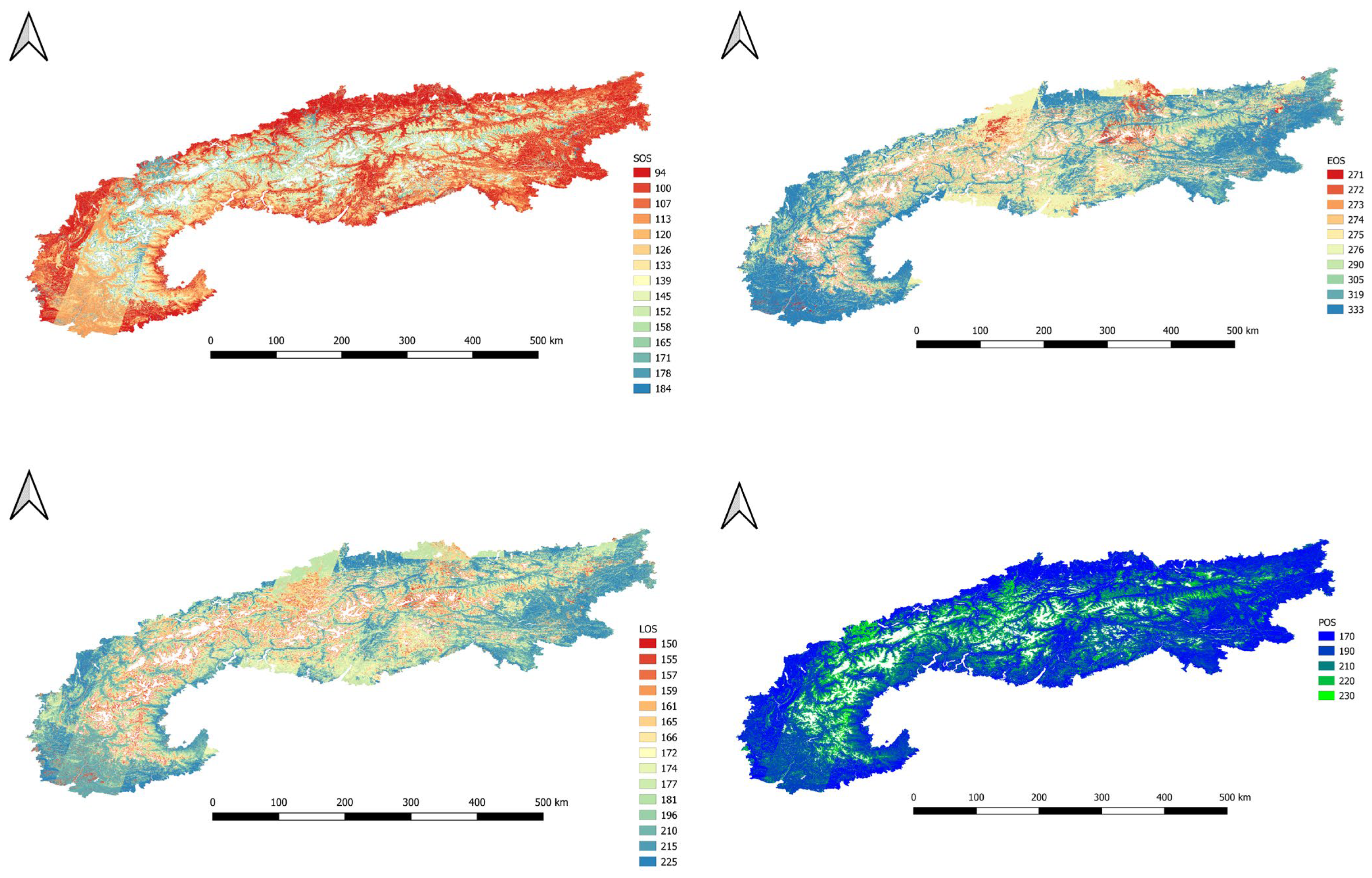
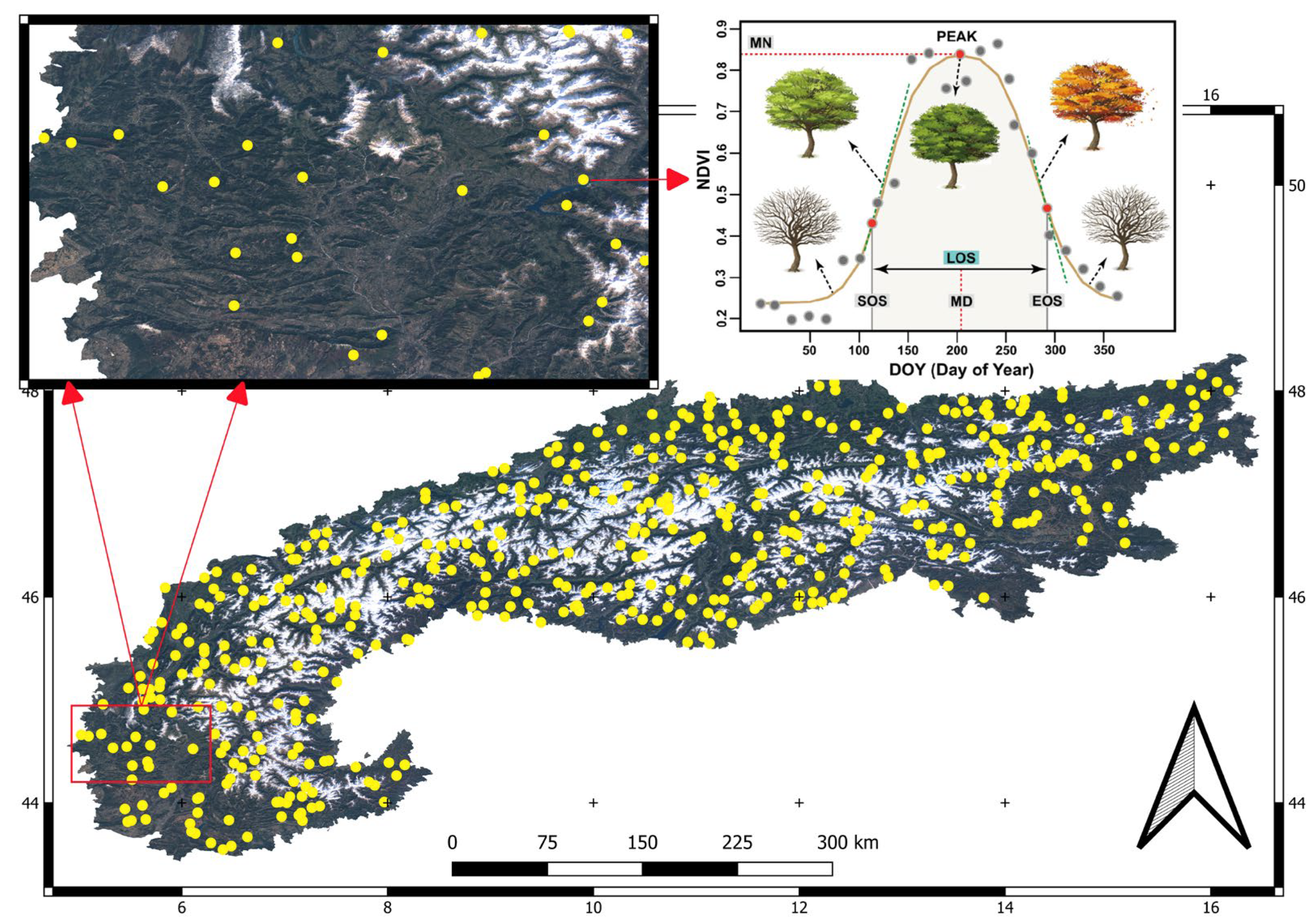
- The start of the season (SOS = Start of Season), indicated with reference to the date (often expressed in the form DOY, day of year) on which vegetative activity is observed to begin in a certain position.
- (b)
- The end of the season (EOS = End of Season), indicated with reference to the date on which the vegetative activity in that position is observed to end.
- (c)
- The length of the season (LOS = Length of Season), defined as the difference in groups between EOS and SOS.
- (d)
- The maximum vegetation index value (MAX_VI), identified between SOS and EOS.
- (e)
- The date on which MAX_VI occurs (MAX_DOY).
- (f)
- The amplitude of the season (SA = Season Amplitude), which defines the difference between the maximum and minimum values of the index in the considered season.
- (g)
- Total productivity (TP = Total Productivity), which defines the integral of the interpolated profile over the entire year.
- (h)
- Seasonal productivity (SP = Seasonal Productivity or SMI = Small Integral), which defines the integral of the interpolated profile of the VI between SOS and EOS.
- (i)
- The rate of increase at the beginning of the season (Rate of Increase), defined, with reference to the growing part of the phenological bell (left), as the difference between the index values corresponding, respectively, to 80% and 20% SA, divided by the corresponding time interval.
- (j)
- The rate of decrease at the end of the season (Rate of Decrease), defined, with reference to the decreasing part of the phenological bell (right), as the absolute value of the difference between the index values corresponding, respectively, to 80% and 20% SA, divided by the corresponding time interval.
2. Materials and Methods
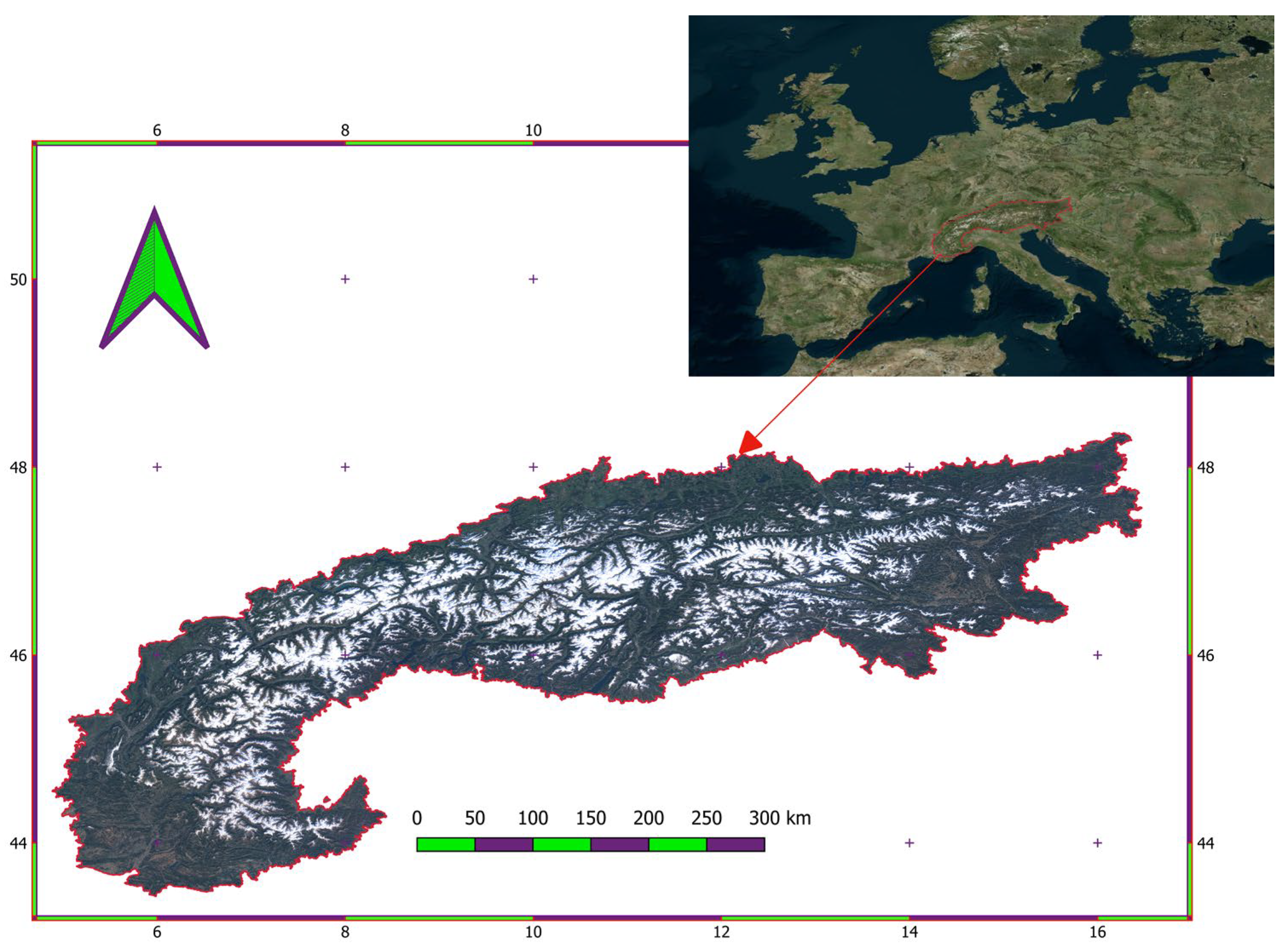
2.1. Development Area
2.2. Earth Observation Data
2.3. Phenological Metrics Computation
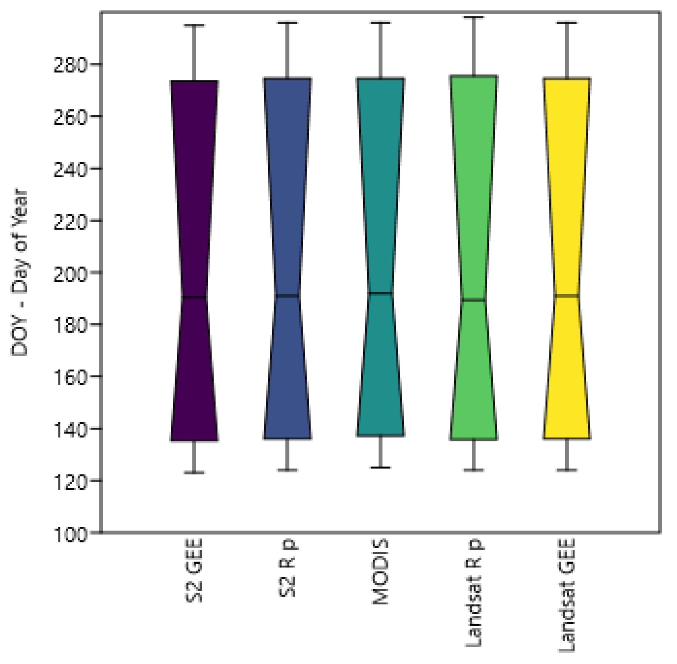
2.4. Algorithm Validation
3. Results
4. Discussion
5. Conclusions
Supplementary Materials
Author Contributions
Funding
Institutional Review Board Statement
Informed Consent Statement
Data Availability Statement
Acknowledgments
Conflicts of Interest
References
- Gorelick, N.; Hancher, M.; Dixon, M.; Ilyushchenko, S.; Thau, D.; Moore, R. Google Earth Engine: Planetary-Scale Geospatial Analysis for Everyone. Remote Sens. Environ. 2017, 202, 18–27. [Google Scholar] [CrossRef]
- Amani, M.; Ghorbanian, A.; Ahmadi, S.A.; Kakooei, M.; Moghimi, A.; Mirmazloumi, S.M.; Moghaddam, S.H.A.; Mahdavi, S.; Ghahremanloo, M.; Parsian, S.; et al. Google Earth Engine Cloud Computing Platform for Remote Sensing Big Data Applications: A Comprehensive Review. IEEE J. Sel. Top. Appl. Earth Obs. Remote Sens. 2020, 13, 5326–5350. [Google Scholar] [CrossRef]
- Kumar, L.; Mutanga, O. Google Earth Engine Applications since Inception: Usage, Trends, and Potential. Remote Sens. 2018, 10, 1509. [Google Scholar] [CrossRef] [Green Version]
- Aybar, C.; Wu, Q.; Bautista, L.; Yali, R.; Barja, A. Rgee: An R Package for Interacting with Google Earth Engine. J. Open Source Softw. 2020, 5, 2272. [Google Scholar] [CrossRef]
- Guo, Y.; Xia, H.; Pan, L.; Zhao, X.; Li, R. Mapping the Northern Limit of Double Cropping Using a Phenology-Based Algorithm and Google Earth Engine. Remote Sens. 2022, 14, 1004. [Google Scholar] [CrossRef]
- Mutanga, O.; Kumar, L. Google Earth Engine Applications. Remote Sens. 2019, 11, 591. [Google Scholar] [CrossRef] [Green Version]
- Orusa, T.; Cammareri, D.; Borgogno Mondino, E. A Possible Land Cover EAGLE Approach to Overcome Remote Sensing Limitations in the Alps Based on Sentinel-1 and Sentinel-2: The Case of Aosta Valley (NW Italy). Remote Sens. 2022, 15, 178. [Google Scholar] [CrossRef]
- Orusa, T.; Cammareri, D.; Borgogno Mondino, E. A Scalable Earth Observation Service to Map Land Cover in Geomorphological Complex Areas beyond the Dynamic World: An Application in Aosta Valley (NW Italy). Appl. Sci. 2022, 13, 390. [Google Scholar] [CrossRef]
- Orusa, T.; Mondino, E.B. Landsat 8 Thermal Data to Support Urban Management and Planning in the Climate Change Era: A Case Study in Torino Area, NW Italy. In Proceedings of the Remote Sensing Technologies and Applications in Urban Environments IV, Strasbourg, France, 9–10 September 2019; International Society for Optics and Photonics. Volume 11157, pp. 133–149. [Google Scholar]
- Carella, E.; Orusa, T.; Viani, A.; Meloni, D.; Borgogno-Mondino, E.; Orusa, R. An Integrated, Tentative Remote-Sensing Approach Based on NDVI Entropy to Model Canine Distemper Virus in Wildlife and to Prompt Science-Based Management Policies. Animals 2022, 12, 1049. [Google Scholar] [CrossRef]
- Zhao, Q.; Yu, L.; Li, X.; Peng, D.; Zhang, Y.; Gong, P. Progress and Trends in the Application of Google Earth and Google Earth Engine. Remote Sens. 2021, 13, 3778. [Google Scholar] [CrossRef]
- Kennedy, R.E.; Yang, Z.; Gorelick, N.; Braaten, J.; Cavalcante, L.; Cohen, W.B.; Healey, S. Implementation of the LandTrendr Algorithm on Google Earth Engine. Remote Sens. 2018, 10, 691. [Google Scholar] [CrossRef] [Green Version]
- Tamiminia, H.; Salehi, B.; Mahdianpari, M.; Quackenbush, L.; Adeli, S.; Brisco, B. Google Earth Engine for Geo-Big Data Applications: A Meta-Analysis and Systematic Review. ISPRS J. Photogramm. Remote Sens. 2020, 164, 152–170. [Google Scholar] [CrossRef]
- Yang, L.; Driscol, J.; Sarigai, S.; Wu, Q.; Chen, H.; Lippitt, C.D. Google Earth Engine and Artificial Intelligence (Ai): A Comprehensive Review. Remote Sens. 2022, 14, 3253. [Google Scholar] [CrossRef]
- Orusa, T.; Borgogno Mondino, E. Exploring Short-Term Climate Change Effects on Rangelands and Broad-Leaved Forests by Free Satellite Data in Aosta Valley (Northwest Italy). Climate 2021, 9, 47. [Google Scholar] [CrossRef]
- Orusa, T.; Orusa, R.; Viani, A.; Carella, E.; Borgogno Mondino, E. Geomatics and EO Data to Support Wildlife Diseases Assessment at Landscape Level: A Pilot Experience to Map Infectious Keratoconjunctivitis in Chamois and Phenological Trends in Aosta Valley (NW Italy). Remote Sens. 2020, 12, 3542. [Google Scholar] [CrossRef]
- Peñuelas, J.; Filella, I. Phenology Feedbacks on Climate Change. Science 2009, 324, 887–888. [Google Scholar] [CrossRef] [Green Version]
- Piao, S.; Liu, Q.; Chen, A.; Janssens, I.A.; Fu, Y.; Dai, J.; Liu, L.; Lian, X.; Shen, M.; Zhu, X. Plant Phenology and Global Climate Change: Current Progresses and Challenges. Glob. Change Biol. 2019, 25, 1922–1940. [Google Scholar] [CrossRef]
- Bolton, D.K.; Gray, J.M.; Melaas, E.K.; Moon, M.; Eklundh, L.; Friedl, M.A. Continental-Scale Land Surface Phenology from Harmonized Landsat 8 and Sentinel-2 Imagery. Remote Sens. Environ. 2020, 240, 111685. [Google Scholar] [CrossRef]
- Yuan, M.; Wang, L.; Lin, A.; Liu, Z.; Qu, S. Variations in Land Surface Phenology and Their Response to Climate Change in Yangtze River Basin during 1982–2015. Theor. Appl. Climatol. 2019, 137, 1659–1674. [Google Scholar] [CrossRef]
- Pourghasemi, H.R.; Pouyan, S.; Heidari, B.; Farajzadeh, Z.; Shamsi, S.R.F.; Babaei, S.; Khosravi, R.; Etemadi, M.; Ghanbarian, G.; Farhadi, A.; et al. Spatial Modeling, Risk Mapping, Change Detection, and Outbreak Trend Analysis of Coronavirus (COVID-19) in Iran (Days between February 19 and June 14, 2020). Int. J. Infect. Dis. 2020, 98, 90–108. [Google Scholar] [CrossRef]
- Borgogno-Mondino, E.; Farbo, A.; Novello, V.; de Palma, L. A Fast Regression-Based Approach to Map Water Status of Pomegranate Orchards with Sentinel 2 Data. Horticulturae 2022, 8, 759. [Google Scholar] [CrossRef]
- Yang, Y.; Qi, N.; Zhao, J.; Meng, N.; Lu, Z.; Wang, X.; Kang, L.; Wang, B.; Li, R.; Ma, J.; et al. Detecting the Turning Points of Grassland Autumn Phenology on the Qinghai-Tibetan Plateau: Spatial Heterogeneity and Controls. Remote Sens. 2021, 13, 4797. [Google Scholar] [CrossRef]
- Chen, F.; Liu, Z.; Zhong, H.; Wang, S. Exploring the Applicability and Scaling Effects of Satellite-Observed Spring and Autumn Phenology in Complex Terrain Regions Using Four Different Spatial Resolution Products. Remote Sens. 2021, 13, 4582. [Google Scholar] [CrossRef]
- Vizzari, M. PlanetScope, Sentinel-2, and Sentinel-1 Data Integration for Object-Based Land Cover Classification in Google Earth Engine. Remote Sens. 2022, 14, 2628. [Google Scholar] [CrossRef]
- De Marinis, P.; De Petris, S.; Sarvia, F.; Manfron, G.; Momo, E.J.; Orusa, T.; Corvino, G.; Sali, G.; Borgogno, E.M. Supporting Pro-Poor Reforms of Agricultural Systems in Eastern DRC (Africa) with Remotely Sensed Data: A Possible Contribution of Spatial Entropy to Interpret Land Management Practices. Land 2021, 10, 1368. [Google Scholar] [CrossRef]
- da Silva Junior, C.A.; Leonel-Junior, A.H.S.; Rossi, F.S.; Correia Filho, W.L.F.; de Barros Santiago, D.; de Oliveira-Júnior, J.F.; Teodoro, P.E.; Lima, M.; Capristo-Silva, G.F. Mapping Soybean Planting Area in Midwest Brazil with Remotely Sensed Images and Phenology-Based Algorithm Using the Google Earth Engine Platform. Comput. Electron. Agric. 2020, 169, 105194. [Google Scholar] [CrossRef]
- dela Torre, D.M.G.; Gao, J.; Macinnis-Ng, C.; Shi, Y. Phenology-Based Delineation of Irrigated and Rain-Fed Paddy Fields with Sentinel-2 Imagery in Google Earth Engine. Geo-Spat. Inf. Sci. 2021, 24, 695–710. [Google Scholar] [CrossRef]
- Kumar, M.; Phukon, S.N.; Paygude, A.C.; Tyagi, K.; Singh, H. Mapping Phenological Functional Types (PhFT) in the Indian Eastern Himalayas Using Machine Learning Algorithm in Google Earth Engine. Comput. Geosci. 2022, 158, 104982. [Google Scholar] [CrossRef]
- Ni, R.; Tian, J.; Li, X.; Yin, D.; Li, J.; Gong, H.; Zhang, J.; Zhu, L.; Wu, D. An Enhanced Pixel-Based Phenological Feature for Accurate Paddy Rice Mapping with Sentinel-2 Imagery in Google Earth Engine. ISPRS J. Photogramm. Remote Sens. 2021, 178, 282–296. [Google Scholar] [CrossRef]
- Guo, Y.; Xia, H.; Pan, L.; Zhao, X.; Li, R.; Bian, X.; Wang, R.; Yu, C. Development of a New Phenology Algorithm for Fine Mapping of Cropping Intensity in Complex Planting Areas Using Sentinel-2 and Google Earth Engine. ISPRS Int. J. Geo-Inf. 2021, 10, 587. [Google Scholar] [CrossRef]
- Pan, L.; Xia, H.; Zhao, X.; Guo, Y.; Qin, Y. Mapping Winter Crops Using a Phenology Algorithm, Time-Series Sentinel-2 and Landsat-7/8 Images, and Google Earth Engine. Remote Sens. 2021, 13, 2510. [Google Scholar] [CrossRef]
- Pan, L.; Xia, H.; Yang, J.; Niu, W.; Wang, R.; Song, H.; Guo, Y.; Qin, Y. Mapping Cropping Intensity in Huaihe Basin Using Phenology Algorithm, All Sentinel-2 and Landsat Images in Google Earth Engine. Int. J. Appl. Earth Obs. Geoinf. 2021, 102, 102376. [Google Scholar] [CrossRef]
- Kibret, K.S.; Marohn, C.; Cadisch, G. Use of MODIS EVI to Map Crop Phenology, Identify Cropping Systems, Detect Land Use Change and Drought Risk in Ethiopia–an Application of Google Earth Engine. Eur. J. Remote Sens. 2020, 53, 176–191. [Google Scholar] [CrossRef]
- Salinero-Delgado, M.; Estévez, J.; Pipia, L.; Belda, S.; Berger, K.; Paredes Gómez, V.; Verrelst, J. Monitoring Cropland Phenology on Google Earth Engine Using Gaussian Process Regression. Remote Sens. 2021, 14, 146. [Google Scholar] [CrossRef] [PubMed]
- Cleland, E.E.; Chuine, I.; Menzel, A.; Mooney, H.A.; Schwartz, M.D. Shifting Plant Phenology in Response to Global Change. Trends Ecol. Evol. 2007, 22, 357–365. [Google Scholar] [CrossRef]
- Carter, S.K.; Saenz, D.; Rudolf, V.H. Shifts in Phenological Distributions Reshape Interaction Potential in Natural Communities. Ecol. Lett. 2018, 21, 1143–1151. [Google Scholar] [CrossRef]
- Sarvia, F.; De Petris, S.; Borgogno-Mondino, E. Exploring Climate Change Effects on Vegetation Phenology by MOD13Q1 Data: The Piemonte Region Case Study in the Period 2001–2019. Agronomy 2021, 11, 555. [Google Scholar] [CrossRef]
- Brown, M.E.; de Beurs, K.; Vrieling, A. The Response of African Land Surface Phenology to Large Scale Climate Oscillations. Remote Sens. Environ. 2010, 114, 2286–2296. [Google Scholar] [CrossRef] [Green Version]
- Beck, P.S.; Atzberger, C.; Høgda, K.A.; Johansen, B.; Skidmore, A.K. Improved Monitoring of Vegetation Dynamics at Very High Latitudes: A New Method Using MODIS NDVI. Remote Sens. Environ. 2006, 100, 321–334. [Google Scholar] [CrossRef]
- Elmore, A.J.; Guinn, S.M.; Minsley, B.J.; Richardson, A.D. Landscape Controls on the Timing of Spring, Autumn, and Growing Season Length in Mid-A Tlantic Forests. Glob. Change Biol. 2012, 18, 656–674. [Google Scholar] [CrossRef] [Green Version]
- White, M.A.; Thornton, P.E.; Running, S.W. A Continental Phenology Model for Monitoring Vegetation Responses to Interannual Climatic Variability. Glob. Biogeochem. Cycles 1997, 11, 217–234. [Google Scholar] [CrossRef]
- Hufkens, K.; Basler, D.; Milliman, T.; Melaas, E.K.; Richardson, A.D. An Integrated Phenology Modelling Framework in R. Methods Ecol. Evol. 2018, 9, 1276–1285. [Google Scholar] [CrossRef] [Green Version]
- Richardson, A.D.; Hufkens, K.; Milliman, T.; Aubrecht, D.M.; Chen, M.; Gray, J.M.; Johnston, M.R.; Keenan, T.F.; Klosterman, S.T.; Kosmala, M.; et al. Tracking Vegetation Phenology across Diverse North American Biomes Using PhenoCam Imagery. Sci. Data 2018, 5, 180028. [Google Scholar] [CrossRef] [PubMed]
- Kong, D. R Package: A State-of-the-Art Vegetation Phenology Extraction Package, Phenofit Version 0.2 6; R Package: Vienna, Austria, 2020. [Google Scholar]
- Kong, D.; Zhang, Y.; Wang, D.; Chen, J.; Gu, X. Photoperiod Explains the Asynchronization between Vegetation Carbon Phenology and Vegetation Greenness Phenology. J. Geophys. Res. Biogeosci. 2020, 125, e2020JG005636. [Google Scholar] [CrossRef]
- Kong, D.; Zhang, Y.; Gu, X.; Wang, D. A Robust Method for Reconstructing Global MODIS EVI Time Series on the Google Earth Engine. ISPRS J. Photogramm. Remote Sens. 2019, 155, 13–24. [Google Scholar] [CrossRef]
- Filippa, G.; Cremonese, E.; Migliavacca, M.; Galvagno, M.; Forkel, M.; Wingate, L.; Tomelleri, E.; Di Cella, U.M.; Richardson, A.D. Phenopix: AR Package for Image-Based Vegetation Phenology. Agric. For. Meteorol. 2016, 220, 141–150. [Google Scholar] [CrossRef] [Green Version]
- Eklundh, L.; Jönsson, P. TIMESAT: A Software Package for Time-Series Processing and Assessment of Vegetation Dynamics. In Remote Sensing Time Series; Springer: Stockholm, Sweden, 2015; pp. 141–158. [Google Scholar]
- Jönsson, P.; Eklundh, L. TIMESAT—A Program for Analyzing Time-Series of Satellite Sensor Data. Comput. Geosci. 2004, 30, 833–845. [Google Scholar] [CrossRef] [Green Version]
- Araya, S.; Ostendorf, B.; Lyle, G.; Lewis, M. CropPhenology: An R Package for Extracting Crop Phenology from Time Series Remotely Sensed Vegetation Index Imagery. Ecol. Inform. 2018, 46, 45–56. [Google Scholar] [CrossRef]
- Beck, P.; Jönsson, P.; Høgda, K.-A.; Karlsen, S.; Eklundh, L.; Skidmore, A. A Ground-Validated NDVI Dataset for Monitoring Vegetation Dynamics and Mapping Phenology in Fennoscandia and the Kola Peninsula. Int. J. Remote Sens. 2007, 28, 4311–4330. [Google Scholar] [CrossRef]
- Armstrong, A.; Ostle, N.J.; Whitaker, J. Solar Park Microclimate and Vegetation Management Effects on Grassland Carbon Cycling. Environ. Res. Lett. 2016, 11, 074016. [Google Scholar] [CrossRef] [Green Version]
- Kohler, T.; Giger, M.; Hurni, H.; Ott, C.; Wiesmann, U.; von Dach, S.W.; Maselli, D. Mountains and Climate Change: A Global Concern. Mt. Res. Dev. 2010, 30, 53–55. [Google Scholar] [CrossRef] [Green Version]
- Adler, C.; Huggel, C.; Orlove, B.; Nolin, A. Climate Change in the Mountain Cryosphere: Impacts and Responses. Reg. Environ. Change 2019, 19, 1225–1228. [Google Scholar] [CrossRef] [Green Version]
- Sarvia, F.; Petris, S.D.; Orusa, T.; Borgogno-Mondino, E. MAIA S2 Versus Sentinel 2: Spectral Issues and Their Effects in the Precision Farming Context. In Proceedings of the International Conference on Computational Science and Its Applications, Cagliari, Italy, 13–16 September 2021; pp. 63–77. [Google Scholar]
- Samuele, D.P.; Filippo, S.; Orusa, T.; Enrico, B.-M. Mapping SAR Geometric Distortions and Their Stability along Time: A New Tool in Google Earth Engine Based on Sentinel-1 Image Time Series. Int. J. Remote Sens. 2021, 42, 9135–9154. [Google Scholar] [CrossRef]
- Meybeck, M.; Green, P.; Vörösmarty, C. A New Typology for Mountains and Other Relief Classes. Mt. Res. Dev. 2001, 21, 34–45. [Google Scholar] [CrossRef] [Green Version]
- Clarke-Sather, A.; Crow-Miller, B.; Banister, J.M.; Anh Thomas, K.; Norman, E.S.; Stephenson, S.R. The Shifting Geopolitics of Water in the Anthropocene. Geopolitics 2017, 22, 332–359. [Google Scholar] [CrossRef]
- Mittermeier, R.A.; Mittermeier, C.G.; Brooks, T.M.; Pilgrim, J.D.; Konstant, W.R.; Da Fonseca, G.A.; Kormos, C. Wilderness and Biodiversity Conservation. Proc. Natl. Acad. Sci. USA 2003, 100, 10309–10313. [Google Scholar] [CrossRef] [Green Version]
- Schlagintweit, H.; Schlagintweit, A. On the Physical Geography of the Alps. 353. Am. J. Sci. 1852, 64, 359. [Google Scholar]
- Deering, D. Measuring” Forage Production” of Grazing Units from Landsat MSS Data. In Proceedings of the Tenth International Symposium of Remote Sensing of the Envrionment, Ann Arbor, MI, USA, 6–10 October 1975; pp. 1169–1198. [Google Scholar]
- Deering, D.W. Rangeland Reflectance Characteristics Measured by Aircraft and Spacecraftsensors; Texas A&M University: College Station, TX, USA, 1978. [Google Scholar]
- Rouse, J.; Haas, R.; Schell, J.; Deering, D. Monitoring vegetation systems in the greant plains with ERTS. In Proceedings of the Third ERTS (Earth Resources Technology Satellite) Symposium, NASA SP-351, Washington, DC, USA, 10–14 December 1973; Volume 1, pp. 309–317. [Google Scholar]
- Rouse, J., Jr.; Haas, R.H.; Deering, D.; Schell, J.; Harlan, J.C. Monitoring the Vernal Advancement and Retrogradation (Green Wave Effect) of Natural Vegetation; Springer: New York, NY, USA, 1974. [Google Scholar]
- Tucker, C.J. Red and Photographic Infrared Linear Combinations for Monitoring Vegetation. Remote Sens. Environ. 1979, 8, 127–150. [Google Scholar] [CrossRef] [Green Version]
- Wang, C.; Li, J.; Liu, Q.; Zhong, B.; Wu, S.; Xia, C. Analysis of Differences in Phenology Extracted from the Enhanced Vegetation Index and the Leaf Area Index. Sensors 2017, 17, 1982. [Google Scholar] [CrossRef] [Green Version]
- Wu, C.; Chen, J.M.; Huang, N. Predicting Gross Primary Production from the Enhanced Vegetation Index and Photosynthetically Active Radiation: Evaluation and Calibration. Remote Sens. Environ. 2011, 115, 3424–3435. [Google Scholar] [CrossRef]
- Liu, Z.; Liu, K.; Zhang, J.; Yan, C.; Lock, T.R.; Kallenbach, R.L.; Yuan, Z. Fractional Coverage Rather than Green Chromatic Coordinate Is a Robust Indicator to Track Grassland Phenology Using Smartphone Photography. Ecol. Inform. 2022, 68, 101544. [Google Scholar] [CrossRef]
- Xu, D.; Wang, C.; Chen, J.; Shen, M.; Shen, B.; Yan, R.; Li, Z.; Karnieli, A.; Chen, J.; Yan, Y.; et al. The Superiority of the Normalized Difference Phenology Index (NDPI) for Estimating Grassland Aboveground Fresh Biomass. Remote Sens. Environ. 2021, 264, 112578. [Google Scholar] [CrossRef]
- Wang, C.; Chen, J.; Wu, J.; Tang, Y.; Shi, P.; Black, T.A.; Zhu, K. A Snow-Free Vegetation Index for Improved Monitoring of Vegetation Spring Green-up Date in Deciduous Ecosystems. Remote Sens. Environ. 2017, 196, 1–12. [Google Scholar] [CrossRef]
- Bórnez, K.; Descals, A.; Verger, A.; Peñuelas, J. Land Surface Phenology from VEGETATION and PROBA-V Data. Assessment over Deciduous Forests. Int. J. Appl. Earth Obs. Geoinf. 2020, 84, 101974. [Google Scholar] [CrossRef]
- Zeng, L.; Wardlow, B.D.; Xiang, D.; Hu, S.; Li, D. A Review of Vegetation Phenological Metrics Extraction Using Time-Series, Multispectral Satellite Data. Remote Sens. Environ. 2020, 237, 111511. [Google Scholar] [CrossRef]
- Van Der Walt, S.; Colbert, S.C.; Varoquaux, G. The NumPy Array: A Structure for Efficient Numerical Computation. Comput. Sci. Eng. 2011, 13, 22–30. [Google Scholar] [CrossRef] [Green Version]
- Kong, D.; McVicar, T.R.; Xiao, M.; Zhang, Y.; Peña-Arancibia, J.L.; Filippa, G.; Xie, Y.; Gu, X. Phenofit: An R Package for Extracting Vegetation Phenology from Time Series Remote Sensing. Methods Ecol. Evol. 2022, 13, 1508–1527. [Google Scholar] [CrossRef]
- Stenseth, N.C.; Mysterud, A. Climate, Changing Phenology, and Other Life History Traits: Nonlinearity and Match–Mismatch to the Environment. Proc. Natl. Acad. Sci. USA 2002, 99, 13379–13381. [Google Scholar] [CrossRef] [PubMed] [Green Version]
- Puchalka, R.; Klisz, M.; Koniakin, S.; Czortek, P.; Dylewski, L.; Paź-Dyderska, S.; Vítková, M.; Sádlo, J.; Rašomavičius, V.; Čarni, A.; et al. Citizen Science Helps Predictions of Climate Change Impact on Flowering Phenology: A Study on Anemone Nemorosa. Agric. For. Meteorol. 2022, 325, 109133. [Google Scholar] [CrossRef]
- Sass-Klaassen, U.; Sabajo, C.R.; den Ouden, J. Vessel Formation in Relation to Leaf Phenology in Pedunculate Oak and European Ash. Dendrochronologia 2011, 29, 171–175. [Google Scholar] [CrossRef]
- Puchalka, R.; Koprowski, M.; Gričar, J.; Przybylak, R. Does Tree-Ring Formation Follow Leaf Phenology in Pedunculate Oak (Quercus Robur L.)? Eur. J. For. Res. 2017, 136, 259–268. [Google Scholar] [CrossRef] [Green Version]
- Matsushita, B.; Yang, W.; Chen, J.; Onda, Y.; Qiu, G. Sensitivity of the Enhanced Vegetation Index (EVI) and Normalized Difference Vegetation Index (NDVI) to Topographic Effects: A Case Study in High-Density Cypress Forest. Sensors 2007, 7, 2636–2651. [Google Scholar] [CrossRef] [PubMed] [Green Version]
- Kumari, N.; Srivastava, A.; Dumka, U.C. A Long-Term Spatiotemporal Analysis of Vegetation Greenness over the Himalayan Region Using Google Earth Engine. Climate 2021, 9, 109. [Google Scholar] [CrossRef]
- Gao, X.; Huete, A.R.; Ni, W.; Miura, T. Optical–Biophysical Relationships of Vegetation Spectra without Background Contamination. Remote Sens. Environ. 2000, 74, 609–620. [Google Scholar] [CrossRef]
- Huete, A.; Didan, K.; Miura, T.; Rodriguez, E.P.; Gao, X.; Ferreira, L.G. Overview of the Radiometric and Biophysical Performance of the MODIS Vegetation Indices. Remote Sens. Environ. 2002, 83, 195–213. [Google Scholar] [CrossRef]
- Yan, E.; Wang, G.; Lin, H.; Xia, C.; Sun, H. Phenology-Based Classification of Vegetation Cover Types in Northeast China Using MODIS NDVI and EVI Time Series. Int. J. Remote Sens. 2015, 36, 489–512. [Google Scholar] [CrossRef]
- Dong, T.; Liu, J.; Qian, B.; Zhao, T.; Jing, Q.; Geng, X.; Wang, J.; Huffman, T.; Shang, J. Estimating Winter Wheat Biomass by Assimilating Leaf Area Index Derived from Fusion of Landsat-8 and MODIS Data. Int. J. Appl. Earth Obs. Geoinf. 2016, 49, 63–74. [Google Scholar] [CrossRef]
- Dong, J.; Xiao, X.; Menarguez, M.A.; Zhang, G.; Qin, Y.; Thau, D.; Biradar, C.; Moore III, B. Mapping Paddy Rice Planting Area in Northeastern Asia with Landsat 8 Images, Phenology-Based Algorithm and Google Earth Engine. Remote Sens. Environ. 2016, 185, 142–154. [Google Scholar] [CrossRef] [PubMed] [Green Version]
- Bagliani, M.M.; Caimotto, M.C.; Latini, G.; Orusa, T. Lessico e Nuvole: Le Parole del Cambiamento Climatico; Università degli studi di Torino: Torino, Italy, 2019. [Google Scholar]
- Latini, G.; Bagliani, M.; Orusa, T. Lessico e Nuvole: Le Parole del Cambiamento Climatico; Università degli studi di Torino Youcanprint: Torino, Italy, 2021. [Google Scholar]


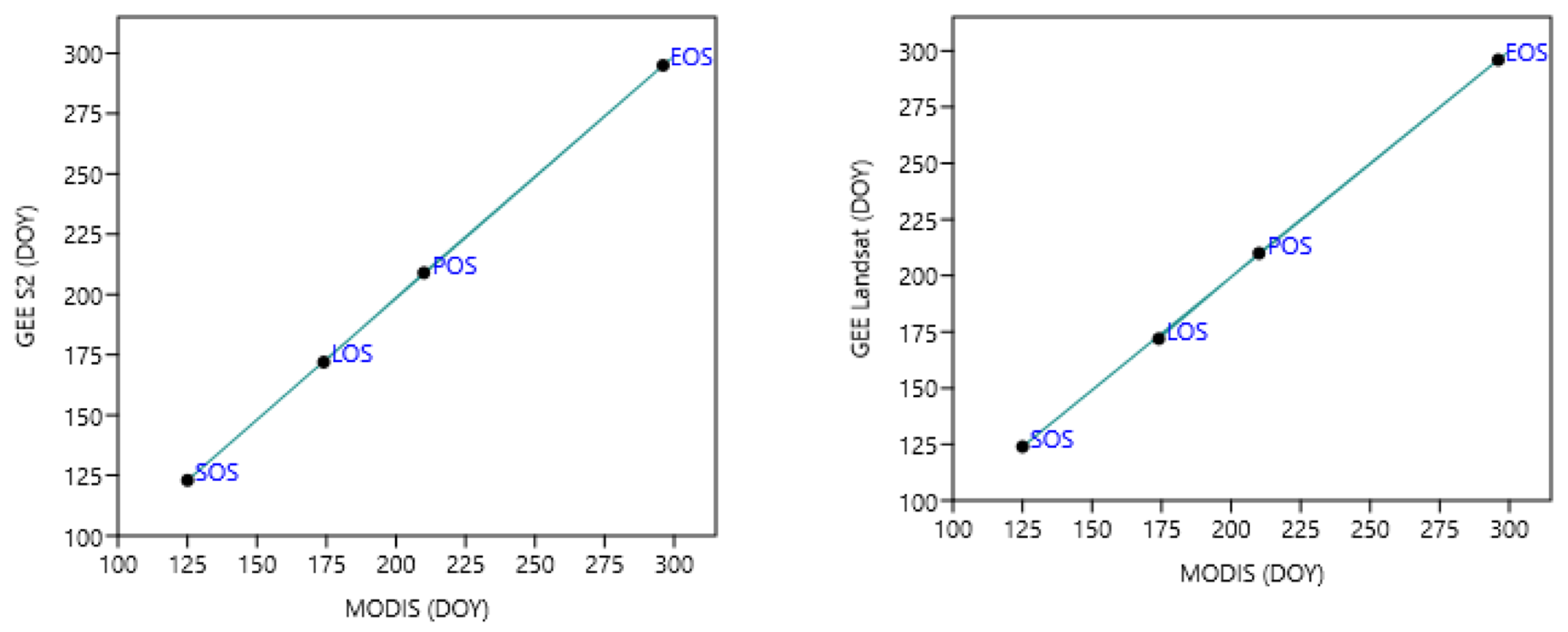
| EO Data and PMs | GEE Algorithm (pi) μ ± σ (DOY) | MODIS Terra and Aqua (oi) μ ± σ (DOY) | MAE | RMSE |
|---|---|---|---|---|
| Sentinel-2 SOS | 123 ± 28 | 125 ± 28 | 2 | 2 |
| Sentinel-2 EOS | 295 ± 34 | 296 ± 34 | 1 | 1 |
| Sentinel-2 POS | 209 ± 18 | 210 ± 18 | 1 | 1 |
| Sentinel-2 LOS | 172 ± 52 | 174 ± 52 | 2 | 2 |
| Landsat 8 SOS | 124 ± 28 | 125 ± 28 | 2 | 2 |
| Landsat 8 EOS | 296 ± 34 | 296 ± 34 | 1 | 1 |
| Landsat 8 POS | 210 ± 18 | 210 ± 18 | 1 | 1 |
| Landsat 8 LOS | 172 ± 52 | 174 ± 52 | 2 | 2 |
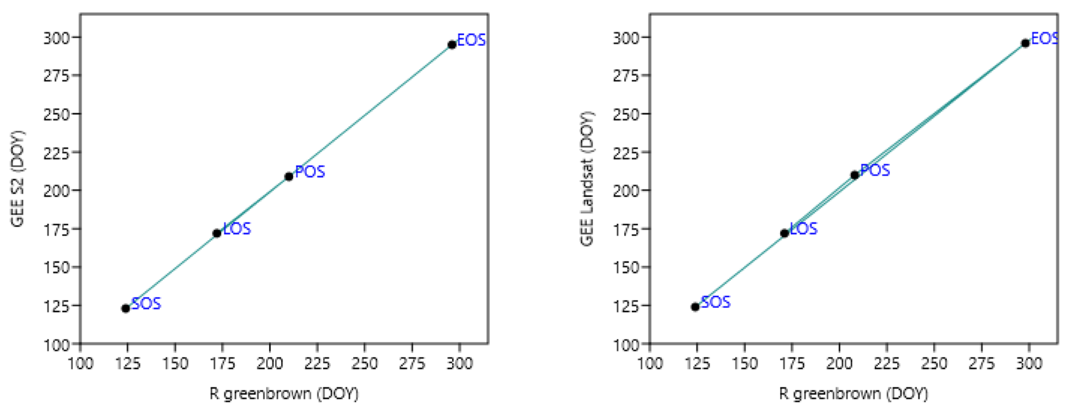
| EO Data and PMs | GEE Algorithm (pi) μ ± σ (DOY) | R Greenbrown Package (oi) μ ± σ (DOY) | MAE | RMSE |
|---|---|---|---|---|
| Sentinel-2 SOS | 123 ± 28 | 124 ± 28 | 1 | 1 |
| Sentinel-2 EOS | 295 ± 34 | 296 ± 34 | 1 | 1 |
| Sentinel-2 POS | 209 ± 18 | 210 ± 18 | 1 | 1 |
| Sentinel-2 LOS | 172 ± 52 | 172 ± 52 | 0 | 0 |
| Landsat 8 SOS | 124 ± 28 | 124 ± 28 | 0 | 0 |
| Landsat 8 EOS | 296 ± 34 | 298 ± 34 | 2 | 2 |
| Landsat 8 POS | 210 ± 18 | 208 ± 18 | 2 | 2 |
| Landsat 8 LOS | 172 ± 52 | 171 ± 52 | 1 | 1 |
Disclaimer/Publisher’s Note: The statements, opinions and data contained in all publications are solely those of the individual author(s) and contributor(s) and not of MDPI and/or the editor(s). MDPI and/or the editor(s) disclaim responsibility for any injury to people or property resulting from any ideas, methods, instructions or products referred to in the content. |
© 2023 by the authors. Licensee MDPI, Basel, Switzerland. This article is an open access article distributed under the terms and conditions of the Creative Commons Attribution (CC BY) license (https://creativecommons.org/licenses/by/4.0/).
Share and Cite
Orusa, T.; Viani, A.; Cammareri, D.; Borgogno Mondino, E. A Google Earth Engine Algorithm to Map Phenological Metrics in Mountain Areas Worldwide with Landsat Collection and Sentinel-2. Geomatics 2023, 3, 221-238. https://doi.org/10.3390/geomatics3010012
Orusa T, Viani A, Cammareri D, Borgogno Mondino E. A Google Earth Engine Algorithm to Map Phenological Metrics in Mountain Areas Worldwide with Landsat Collection and Sentinel-2. Geomatics. 2023; 3(1):221-238. https://doi.org/10.3390/geomatics3010012
Chicago/Turabian StyleOrusa, Tommaso, Annalisa Viani, Duke Cammareri, and Enrico Borgogno Mondino. 2023. "A Google Earth Engine Algorithm to Map Phenological Metrics in Mountain Areas Worldwide with Landsat Collection and Sentinel-2" Geomatics 3, no. 1: 221-238. https://doi.org/10.3390/geomatics3010012