
Prediction of Performance and Geometrical Parameters of Single-Phase Ejectors Using Artificial Neural Networks

 , ,
, ,
Abstract
:1. Introduction
2. Materials and Methods
2.1. Artificial Neural Networks
2.2. Database Description
- Only experimental data from HDRC, including single-phase ejectors, were collected;
- The working fluids are R134a, R245fa, R141b, R1234ze(E) and R1233zd(E). No mixture is considered.
2.3. Construction of the ANN Models
2.4. Training
2.5. Model Validation
3. Results
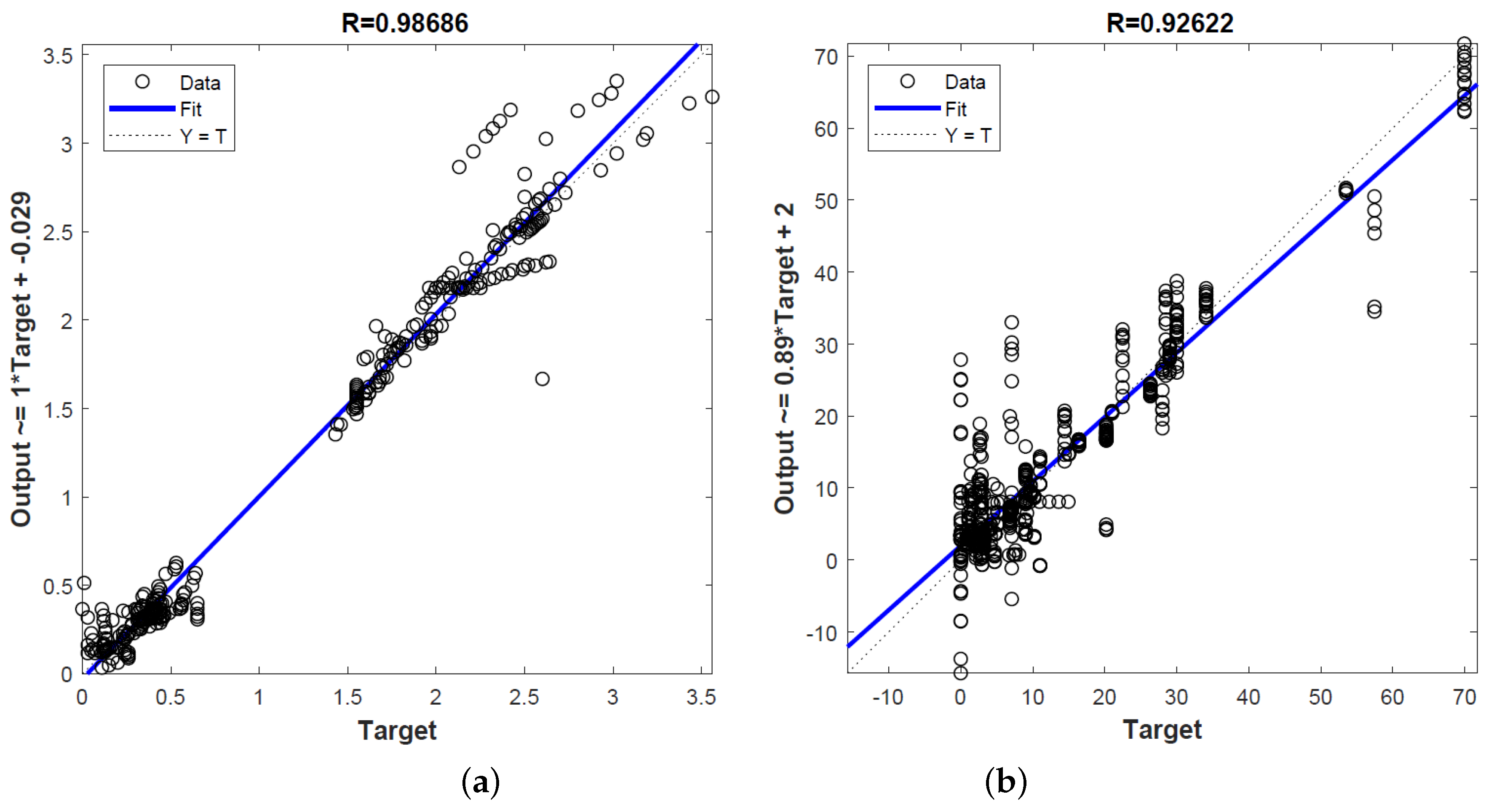
3.1. Generalization Capacity
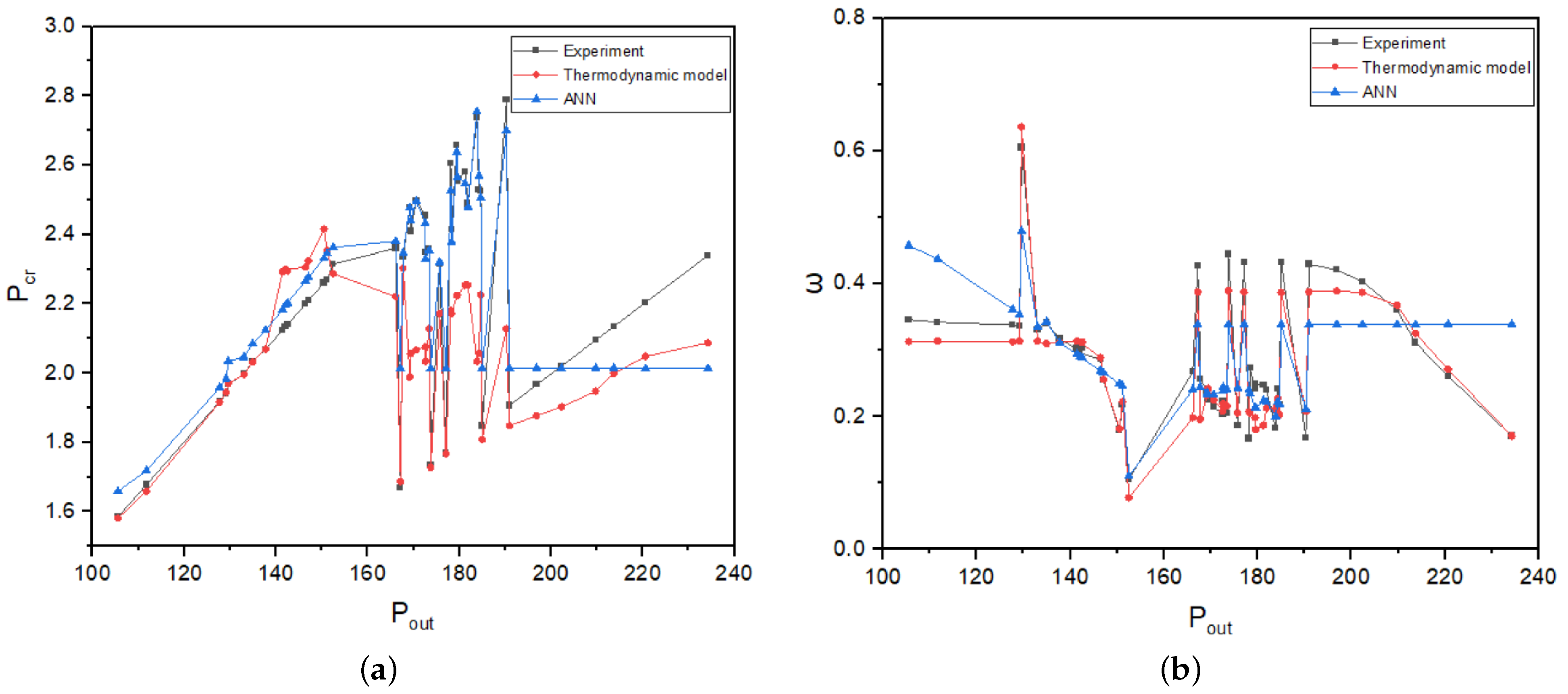
3.2. Operating Conditions
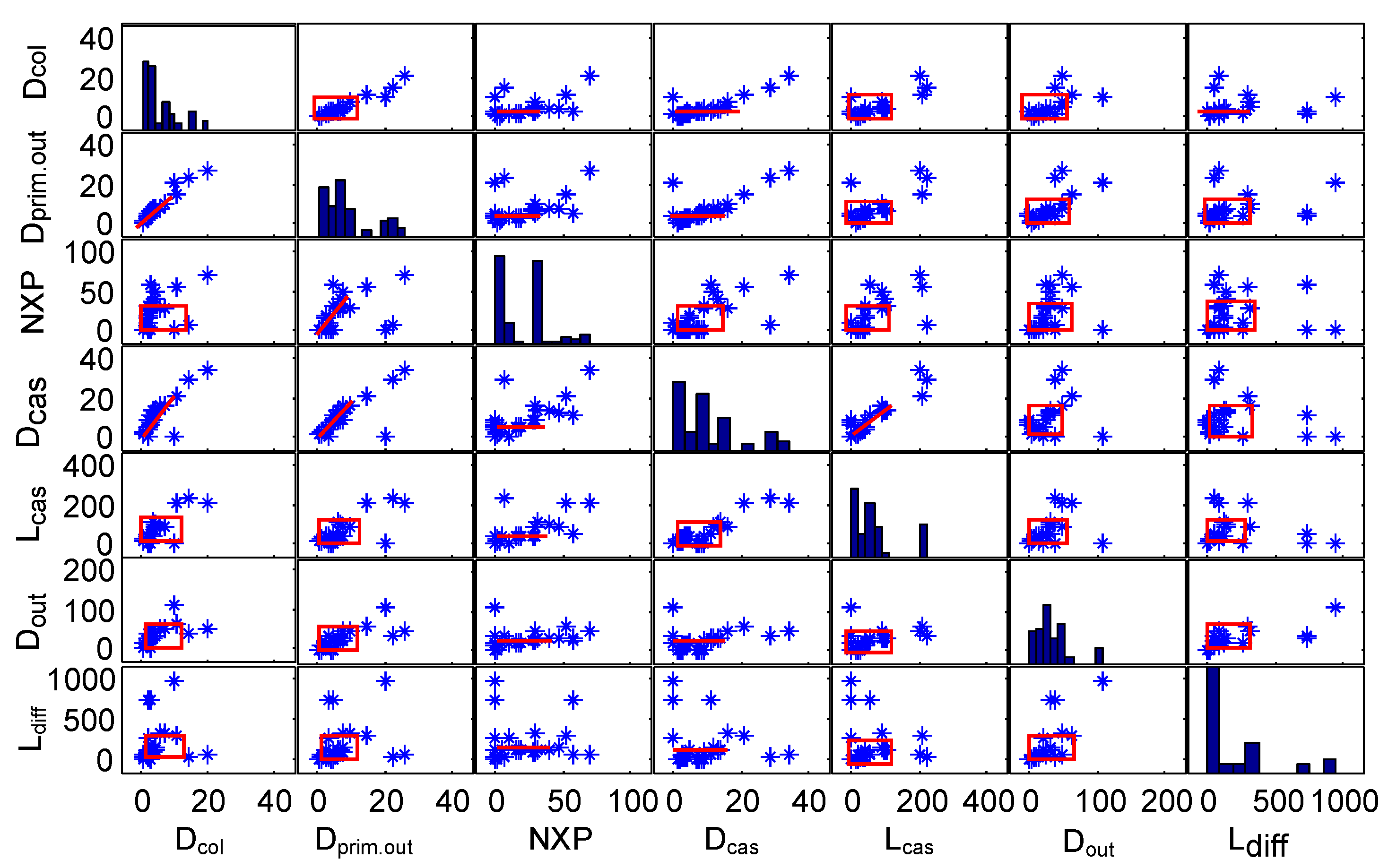
3.3. Importance of Parameters
4. Conclusions
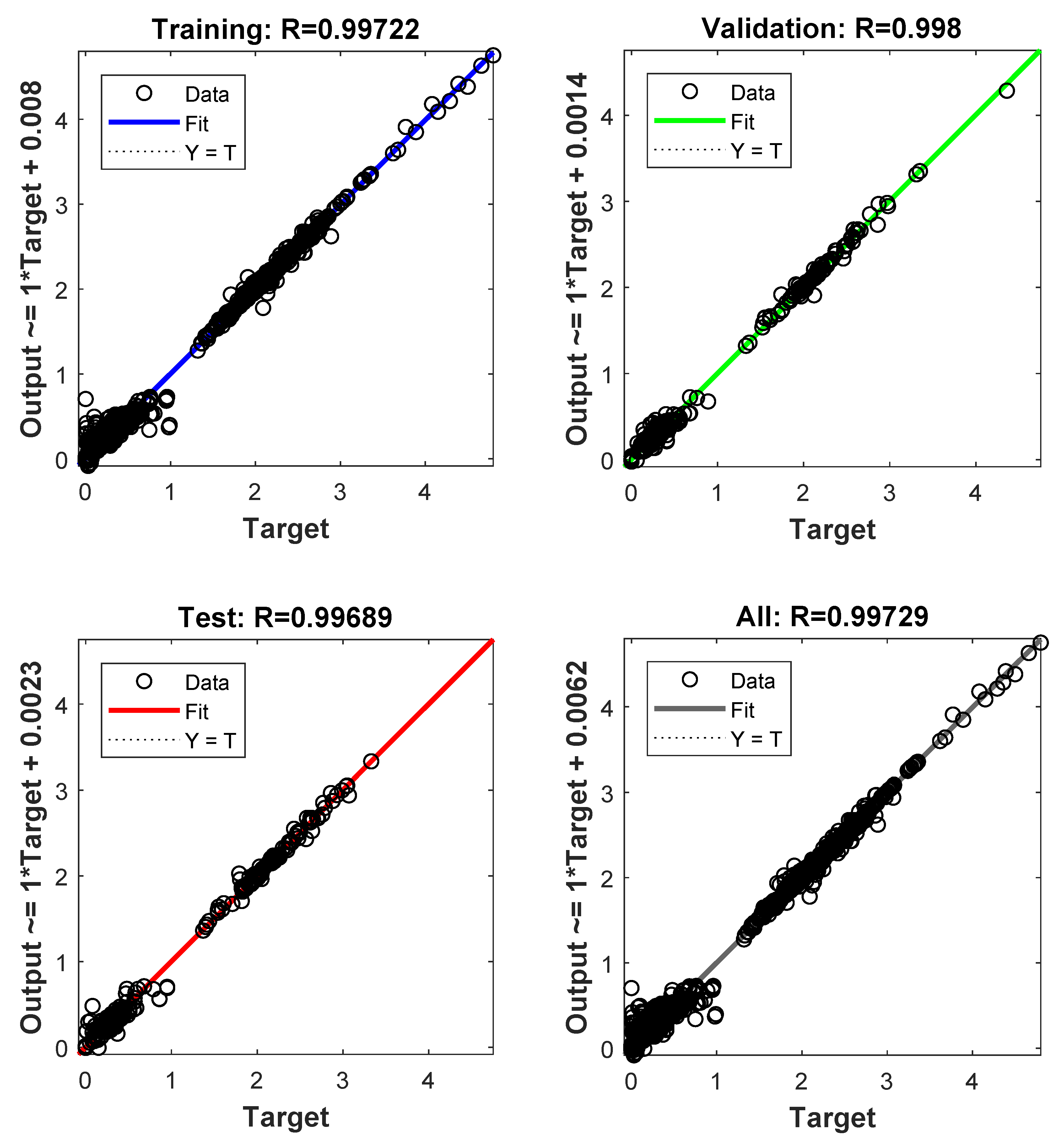
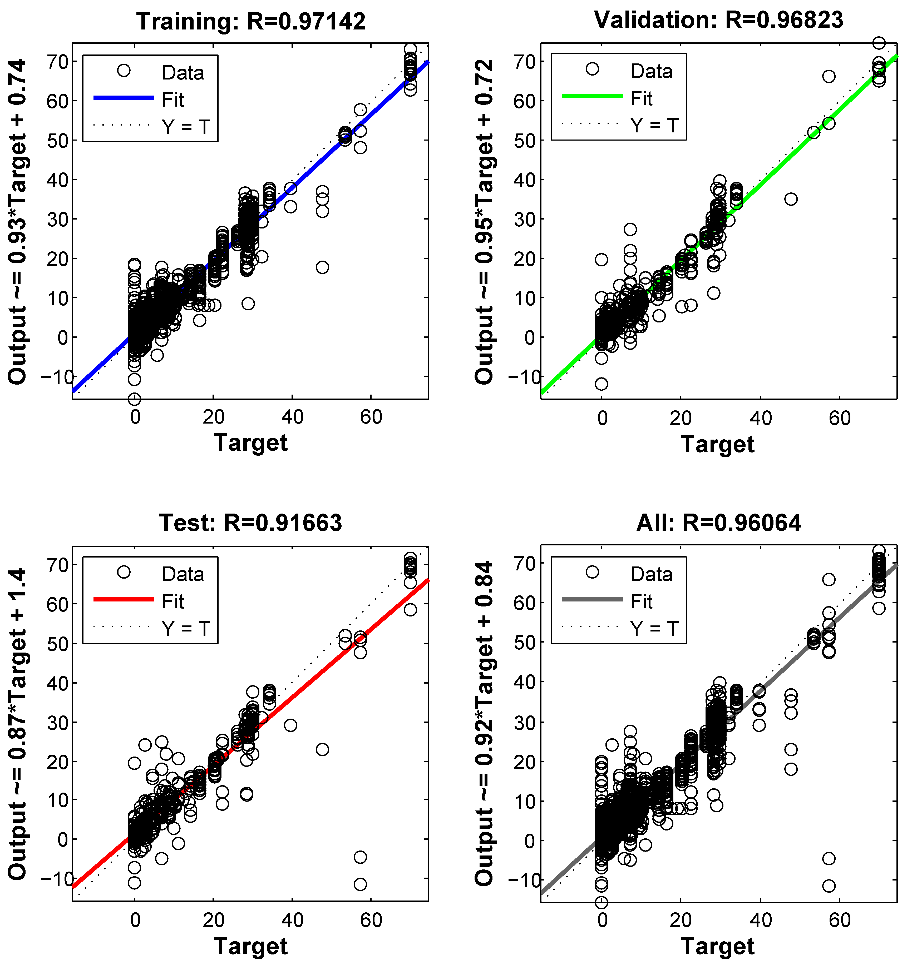
- Both approaches (Cases 1 and 2) show good accuracy. The maximum relative error for both models on the training set was less than 10%. Moreover, Case 1 absolute fractions of variance on the training and test dataset were, respectively, R = 0.9972 and R = 0.9968. For Case 2, the corresponding coefficients were, respectively, R = 0.9714 and R = 0.9166.
- When presented with a dataset of 159 new instances, models show absolute fractions of variance R = 0.9868 (Case 1) and R = 0.9262 (Case 2). This shows the high capacity of the models to predict newly presented data within their training range.
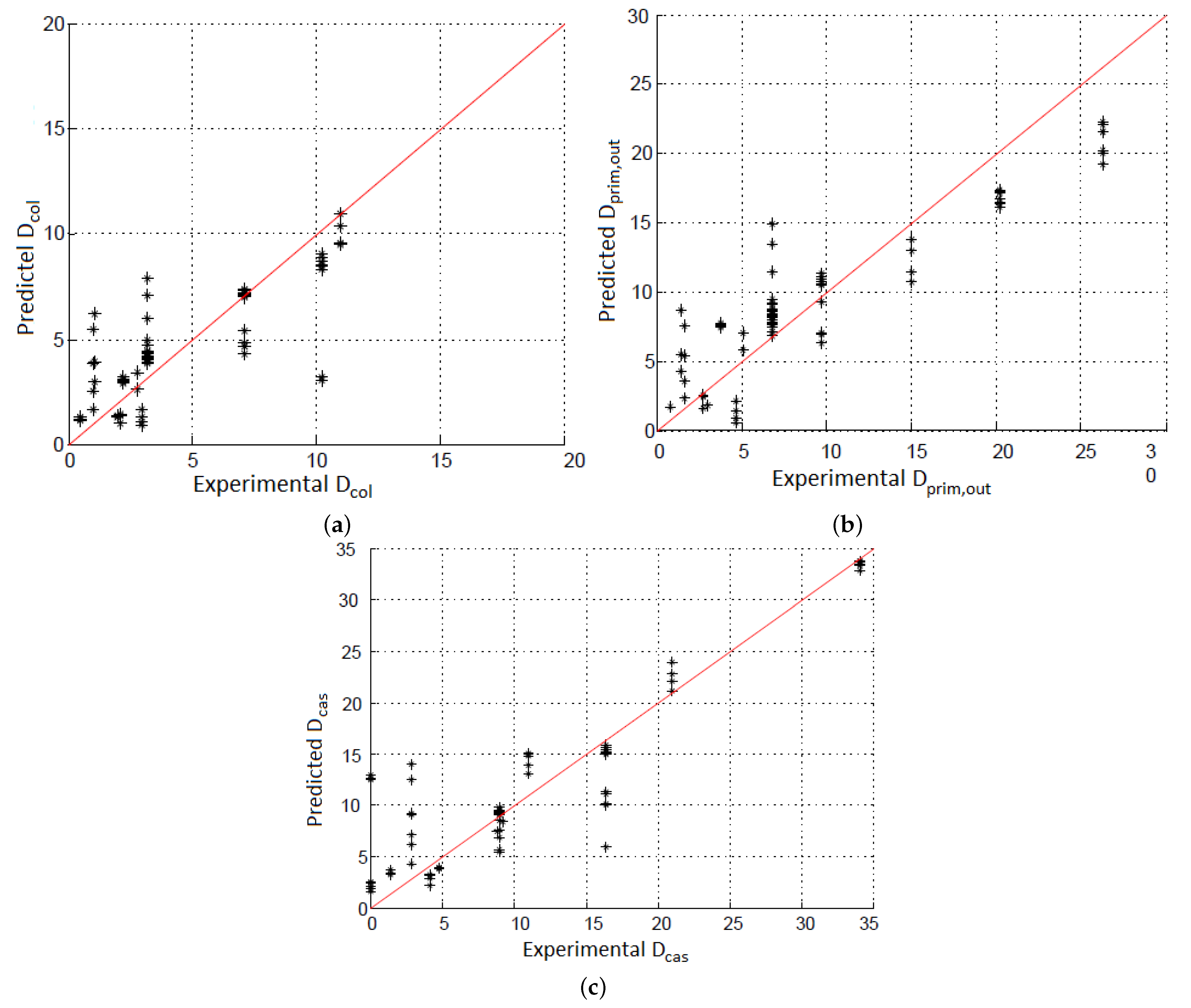
- Comparison between on-design and off-design with 159 data indicates that the two models agree very well with the experimental data. Otherwise, the critical mode offers better results than the sub-critical mode for both operating conditions and geometrical characteristics.
- The most important parameters in the prediction of the ejector performance are the operating conditions for the secondary inlet and outlet, followed by NXP and the primary inlet conditions. Whereas the primary and secondary inlet conditions are the most influential parameters for the estimation of geometrical parameters (, , NXP and ).
- Comparisons with experimental and numerical data show that the ANN can provide better accuracy over a wide range of data.
Author Contributions
Funding
Institutional Review Board Statement
Informed Consent Statement
Data Availability Statement
Acknowledgments
Conflicts of Interest
References
- Aidoun, Z.; Ameur, K.; Falsafioon, M.; Badache, M. Current Advances in Ejector Modeling, Experimentation and Applications for Refrigeration and Heat Pumps. Part 1: Single-Phase Ejectors. Inventions 2019, 4, 15. [Google Scholar] [CrossRef] [Green Version]
- Chen, J.; Jarall, S.; Havtun, H.; Palm, B. A review on versatile ejector applications in refrigeration systems. Renew. Sustain. Energy Rev. 2015, 49, 67–90. [Google Scholar] [CrossRef]
- Lawrence, N.; Elbel, S. Analysis of two-phase ejector performance metrics and comparison of R134a and CO2 ejector performance. Sci. Technol. Built Environ. 2015, 21, 515–525. [Google Scholar] [CrossRef]
- Chunnanond, K.; Aphornratana, S. An experimental investigation of a steam ejector refrigerator: The analysis of the pressure profile along the ejector. Appl. Therm. Eng. 2004, 24, 311–322. [Google Scholar] [CrossRef]
- Hamzaoui, M.; Nesreddine, H.; Aidoun, Z.; Balistrou, M. Experimental study of a low grade heat driven ejector cooling system using the working fluid R245fa. Int. J. Refrig. 2018, 86, 388–400. [Google Scholar] [CrossRef]
- Thongtip, T.; Aphornratana, S. An experimental analysis of the impact of primary nozzle geometries on the ejector performance used in R141b ejector refrigerator. Appl. Therm. Eng. 2017, 110, 89–101. [Google Scholar] [CrossRef]
- Dong, J.; Hu, Q.; Yu, M.; Han, Z.; Cui, W.; Liang, D.; Ma, H.; Pan, X. Numerical investigation on the influence of mixing chamber length on steam ejector performance. Appl. Therm. Eng. 2020, 174, 115204. [Google Scholar] [CrossRef]
- Rao, S.M.; Jagadeesh, G. Observations on the non-mixed length and unsteady shock motion in a two dimensional supersonic ejector. Phys. Fluids 2014, 26, 036103. [Google Scholar] [CrossRef]
- Rand, C.P.; Croquer, S.; Poirier, M.; Poncet, S. Optimal nozzle exit position for a single-phase ejector (Experimental, numerical and thermodynamic modelling). Int. J. Refrig. 2022, 144, 108–117. [Google Scholar] [CrossRef]
- Eames, I.; Wu, S.; Worall, M.; Aphornratana, S. An experimental investigation of steam ejectors for applications in jet-pump refrigerators powered by low-grade heat. Proc. Inst. Mech. Eng. Part A J. Power Energy 1999, 213, 351–361. [Google Scholar] [CrossRef]
- Rao, S.M.; Jagadeesh, G. Novel supersonic nozzles for mixing enhancement in supersonic ejectors. Appl. Therm. Eng. 2014, 71, 62–71. [Google Scholar] [CrossRef]
- García del Valle, J.; Saíz Jabardo, J.; Castro Ruiz, F.; San José Alonso, J. An experimental investigation of a R134a ejector refrigeration system. Int. J. Refrig. 2014, 46, 105–113. [Google Scholar] [CrossRef]
- Galanis, N.; Sorin, M. Ejector design and performance prediction. Int. J. Therm. Sci. 2016, 104, 315–329. [Google Scholar] [CrossRef]
- Huang, B.; Chang, J.; Wang, C.; Petrenko, V. A 1-D analysis of ejector performance. Int. J. Refrig. 1999, 22, 354–364. [Google Scholar] [CrossRef]
- Bilir Sag, N.; Ersoy, H.; Hepbasli, A.; Halkaci, H. Energetic and exergetic comparison of basic and ejector expander refrigeration systems operating under the same external conditions and cooling capacities. Energy Convers. Manag. 2015, 90, 184–194. [Google Scholar] [CrossRef]
- Ringstad, K.E.; Banasiak, K.; Ervik, Å.; Hafner, A. Machine learning and CFD for mapping and optimization of CO2 ejectors. Appl. Therm. Eng. 2021, 199, 117604. [Google Scholar] [CrossRef]
- Besagni, G.; Cristiani, N.; Croci, L.; Guédon, G.R.; Inzoli, F. Computational fluid-dynamics modelling of supersonic ejectors: Screening of modelling approaches, comprehensive validation and assessment of ejector component efficiencies. Appl. Therm. Eng. 2021, 186, 116431. [Google Scholar] [CrossRef]
- Croquer, S.; Poncet, S.; Aidoun, Z. Turbulence modeling of a single-phase R134a supersonic ejector. Part 2: Local flow structure and exergy analysis. Int. J. Refrig. 2016, 61, 153–165. [Google Scholar] [CrossRef]
- Croquer, S.; Lamberts, O.; Poncet, S.; Moreau, S.; Bartosiewicz, Y. Large Eddy Simulation of a supersonic air ejector. Appl. Therm. Eng. 2022, 209, 118177. [Google Scholar] [CrossRef]
- Lamberts, O.; Chatelain, P.; Bartosiewicz, Y. New methods for analyzing transport phenomena in supersonic ejectors. Int. J. Heat Fluid Flow 2017, 64, 23–40. [Google Scholar] [CrossRef]
- Haykin, S. Neural Networks: A Comprehensive Foundation; Prentice Hall PTR: Hoboken, NJ, USA, 1994. [Google Scholar]
- Sözen, A.; Akçayol, M.A. Modelling (using artificial neural-networks) the performance parameters of a solar-driven ejector-absorption cycle. Appl. Energy 2004, 79, 309–325. [Google Scholar] [CrossRef]
- Sözen, A.; Arcaklioğlu, E. Exergy analysis of an ejector-absorption heat transformer using artificial neural network approach. Appl. Therm. Eng. 2007, 27, 481–491. [Google Scholar] [CrossRef]
- Wang, H.; Cai, W.; Wang, Y. Modeling of a hybrid ejector air conditioning system using artificial neural networks. Energy Convers. Manag. 2016, 127, 11–24. [Google Scholar] [CrossRef]
- Rashidi, M.; Aghagoli, A.; Raoofi, R. Thermodynamic analysis of the ejector refrigeration cycle using the artificial neural network. Energy 2017, 129, 201–215. [Google Scholar] [CrossRef]
- Gupta, P.; Kumar, P.; Rao, S.M. Artificial neural network model for single-phase real gas ejectors. Appl. Therm. Eng. 2022, 201, 117615. [Google Scholar] [CrossRef]
- Gupta, P.; Kumar, P.; Rao, S.M. Artificial neural network based shape optimization of supersonic ejectors in the critical flow regime. Appl. Therm. Eng. 2022, 216, 119046. [Google Scholar] [CrossRef]
- Zhang, K.; Zhang, Z.; Han, Y.; Gu, Y.; Qiu, Q.; Zhu, X. Artificial neural network modeling for steam ejector design. Appl. Therm. Eng. 2022, 204, 117939. [Google Scholar] [CrossRef]
- Zheng, J.; Hou, Y.; Tian, Z.; Jiang, H.; Chen, W. Simulation Analysis of Ejector Optimization for High Mass Entrainment under the Influence of Multiple Structural Parameters. Energies 2022, 15, 7058. [Google Scholar] [CrossRef]
- Haykin, S. Self-organizing maps. In Neural Networks—A Comprehensive Foundation, 2nd ed.; Prentice-Hall: Hoboken, NJ, USA, 1999. [Google Scholar]
- Trabelsi, S.; Hafid, M.; Poncet, S.; Poirier, M.; Lacroix, M. Rheology of ethylene-and propylene-glycol ice slurries: Experiments and ANN model. Int. J. Refrig. 2017, 82, 447–460. [Google Scholar] [CrossRef]
- Karami, H.; Ardeshir, A.; Saneie, M.; Salamatian, S.A. Prediction of time variation of scour depth around spur dikes using neural networks. J. Hydroinform. 2011, 14, 180–191. [Google Scholar] [CrossRef]
- Akdag, U.; Komur, M.A.; Ozguc, A.F. Estimation of heat transfer in oscillating annular flow using artifical neural networks. Adv. Eng. Softw. 2009, 40, 864–870. [Google Scholar] [CrossRef]
- Selvaraju, A.; Mani, A. Experimental investigation on R134a vapour ejector refrigeration system. Int. J. Refrig. 2006, 29, 1160–1166. [Google Scholar] [CrossRef]
- Yan, J.; Chen, G.; Liu, C.; Tang, L.; Chen, Q. Experimental investigations on a R134a ejector applied in a refrigeration system. Appl. Therm. Eng. 2017, 110, 1061–1065. [Google Scholar] [CrossRef]
- Li, F.; Li, R.; Li, X.; Tian, Q. Experimental investigation on a R134a ejector refrigeration system under overall modes. Appl. Therm. Eng. 2018, 137, 784–791. [Google Scholar] [CrossRef]
- Poirier, M.; Giguère, D.; Sapoundjiev, H. Experimental parametric investigation of vapor ejector for refrigeration applications. Energy 2018, 162, 1287–1300. [Google Scholar] [CrossRef]
- Falat, A.; Poirier, M.; Sorin, M.; Teyssedou, A. Experimental study of the performance of an ejector system using Freon 134a. Exp. Therm. Fluid Sci. 2019, 105, 165–180. [Google Scholar] [CrossRef]
- Haghparast, P.; Sorin, M.V.; Nesreddine, H. Effects of component polytropic efficiencies on the dimensions of monophasic ejectors. Energy Convers. Manag. 2018, 162, 251–263. [Google Scholar] [CrossRef]
- Haghparast, P.; Sorin, M.V.; Nesreddine, H. The impact of internal ejector working characteristics and geometry on the performance of a refrigeration cycle. Energy 2018, 162, 728–743. [Google Scholar] [CrossRef]
- Shestopalov, K.; Huang, B.; Petrenko, V.; Volovyk, O. Investigation of an experimental ejector refrigeration machine operating with refrigerant R245fa at design and off-design working conditions. Part 2. Theoretical and experimental results. Int. J. Refrig. 2015, 55, 212–223. [Google Scholar] [CrossRef]
- Mazzelli, F.; Milazzo, A. Performance analysis of a supersonic ejector cycle working with R245fa. Int. J. Refrig. 2015, 49, 79–92. [Google Scholar] [CrossRef]
- Scott, D.; Aidoun, Z.; Ouzzane, M. An experimental investigation of an ejector for validating numerical simulations. Int. J. Refrig. 2011, 34, 1717–1723. [Google Scholar] [CrossRef]
- Eames, I.W.; Ablwaifa, A.E.; Petrenko, V. Results of an experimental study of an advanced jet-pump refrigerator operating with R245fa. Appl. Therm. Eng. 2007, 27, 2833–2840. [Google Scholar] [CrossRef]
- Eames, I.W.; Milazzo, A.; Paganini, D.; Livi, M. The design, manufacture and testing of a jet-pump chiller for air conditioning and industrial application. Appl. Therm. Eng. 2013, 58, 234–240. [Google Scholar] [CrossRef]
- Narimani, E.; Sorin, M.; Micheau, P.; Nesreddine, H. Numerical and experimental investigation of the influence of generating pressure on the performance of a one-phase ejector installed within an R245fa refrigeration cycle. Appl. Therm. Eng. 2019, 157, 113654. [Google Scholar] [CrossRef]
- Bencharif, M.; Nesreddine, H.; Croquer, S.; Poncet, S.; Zid, S. The benefit of droplet injection on the performance of an ejector refrigeration cycle working with R245fa. Int. J. Refrig. 2020, 113, 276–287. [Google Scholar] [CrossRef]
- Thongtip, T.; Aphornratana, S. Development and performance of a heat driven R141b ejector air conditioner: Application in hot climate country. Energy 2018, 160, 556–572. [Google Scholar] [CrossRef]
- Ruangtrakoon, N.; Thongtip, T. An experimental investigation to determine the optimal heat source temperature for R141b ejector operation in refrigeration cycle. Appl. Therm. Eng. 2020, 170, 114841. [Google Scholar] [CrossRef]
- Gagan, J.; Śmierciew, K.; Butrymowicz, D. Performance of ejection refrigeration system operating with R-1234ze (E) driven by ultra-low grade heat source. Int. J. Refrig. 2018, 88, 458–471. [Google Scholar] [CrossRef]
- Mahmoudian, J.; Mazzelli, F.; Rocchetti, A.; Milazzo, A. A heat-powered ejector chiller working with low-GWP fluid R1233zd(E) (Part2: Numerical analysis). Int. J. Refrig. 2021, 121, 216–227. [Google Scholar] [CrossRef]
- Buhmann, M.; Dyn, N. Spectral convergence of multiquadric interpolation. Proc. Edinb. Math. Soc. 1993, 36, 319–333. [Google Scholar] [CrossRef]
- Rafiq, M.; Bugmann, G.; Easterbrook, D. Neural network design for engineering applications. Comput. Struct. 2001, 79, 1541–1552. [Google Scholar] [CrossRef]
- Kayabasi, E.; Ozturk, S.; Celik, E.; Kurt, H.; Arcaklioğlu, E. Prediction of nano etching parameters of silicon wafer for a better energy absorption with the aid of an artificial neural network. Sol. Energy Mater. Sol. Cells 2018, 188, 234–240. [Google Scholar] [CrossRef]
- Mathworks, T. Matlab Optimization Toolbox User’s Guide; MathWorks, Inc.: Natick, MA, USA, 2007. [Google Scholar]
- Croquer, S.; Poncet, S.; Aidoun, Z. Thermodynamic modelling of supersonic gas ejector with droplets. Entropy 2017, 19, 579. [Google Scholar] [CrossRef]


| Working Fluid | Reference | Number of Data Points |
|---|---|---|
| R134a | Selvaraju and Mani [34] | 360 |
| García del Valle et al. [12] | ||
| Yan et al. [35] | ||
| Li et al. [36] | ||
| Poirier et al. [37] | ||
| Falat et al. [38] | ||
| R245fa | Haghparast et al. [39,40] | 247 |
| Hamzaoui et al. [5] | ||
| Shestopalov et al. [41] | ||
| Mazzelli and Milazzo [42] | ||
| Scott et al. [43] | ||
| Eames et al. [44,45] | ||
| Narimani et al. [46] | ||
| Bencharif et al. [47] | ||
| R141b | Huang et al. [14] | 264 |
| Thongtip and Aphornratana [6,48] | ||
| Ruangtrakoon and Thongtip [49] | ||
| R1234ze(E)-R1233zd(E) | Gagan et al. [50] | 88 |
| Mahmoudian et al. [51] |
| Parameter | Units | Minimum | Maximum | Mean | Missing Values (%) |
|---|---|---|---|---|---|
| Geometrical Parameters | |||||
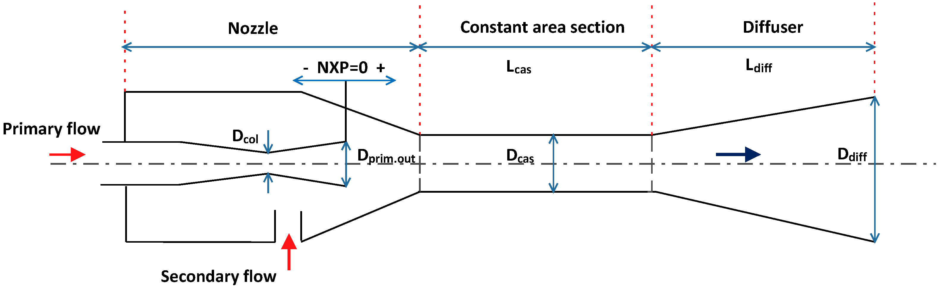
| Primary nozzle throat diameter () | mm | 0.50 | 20.20 | 5.68 | 0% |
| Primary nozzle outlet diameter () | mm | 0.80 | 26.32 | 9.13 | 0% |
| Nozzle exit position (NXP) | mm | 0.00 | 69.93 | 18.55 | 0% |
| Constant area section diameter () | mm | 0 | 34.07 | 10.46 | 0% |
| Constant area section length () | mm | 0 | 223.77 | 69.21 | 4% |
| Diffuser oulet diameter () | mm | 2.60 | 108.30 | 34.91 | 4% |
| Diffuser length () | mm | 11.50 | 950.00 | 212.39 | 4% |
| Operating parameters | |||||
| Primary flow temperature () | ∘C | 48 | 120 | 88.91 | 0% |
| Primary flow pressure () | kPa | 400 | 3907.93 | 1514.13 | 0% |
| Secondary flow temperature () | ∘C | −7 | 30.60 | 9.98 | 0% |
| Secondary flow pressure () | kPa | 20.50 | 630.00 | 195.72 | 0% |
| Condenser temperature () | ∘C | 11.93 | 42.50 | 30.64 | 0% |
| Performance parameters | |||||
| Double-choke entrainment ratio () | - | 0.01 | 0.99 | 0.33 | 3.54% |
| Limiting compression ratio () | - | 0.21 | 4.80 | 2.14 | 0% |
| ANN Model | Input Parameters | Output Parameters |
|---|---|---|
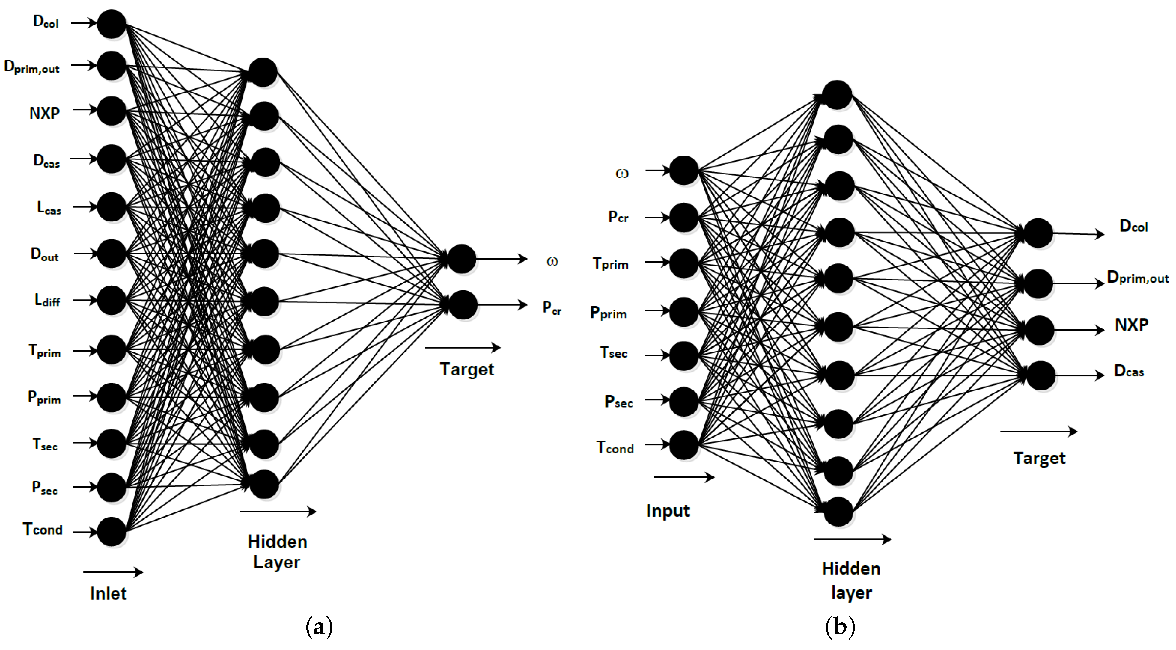
| Case 1: Ejector performance prediction | , , NXP | , |
| , , , | ||
| , , , , | ||
| Case 2: Geometry determination | , , , | , , NXP, |
| , , |
| Parameters/Functions | Value |
|---|---|
| Algorithm | Levenberg–Marquardt |
| Transfer function | Tangent sigmoid |
| Performance parameters | Mean squared error |
| Number of hidden layers | 10 |
| Number of input layers | Case 1 (12) |
| Case 2 (7) | |
| Number of output layers | Case 1 (2) |
| Case 2 (4) | |
| Kinds of samples | Training 70 %, validation 15% and testing 15% |
| Train epoch | Dividerand |
Disclaimer/Publisher’s Note: The statements, opinions and data contained in all publications are solely those of the individual author(s) and contributor(s) and not of MDPI and/or the editor(s). MDPI and/or the editor(s) disclaim responsibility for any injury to people or property resulting from any ideas, methods, instructions or products referred to in the content. |
© 2022 by the authors. Licensee MDPI, Basel, Switzerland. This article is an open access article distributed under the terms and conditions of the Creative Commons Attribution (CC BY) license (https://creativecommons.org/licenses/by/4.0/).
Share and Cite
Bencharif, M.; Croquer, S.; Fang, Y.; Poncet, S.; Nesreddine, H.; Zid, S. Prediction of Performance and Geometrical Parameters of Single-Phase Ejectors Using Artificial Neural Networks. Thermo 2023, 3, 1-20. https://doi.org/10.3390/thermo3010001
Bencharif M, Croquer S, Fang Y, Poncet S, Nesreddine H, Zid S. Prediction of Performance and Geometrical Parameters of Single-Phase Ejectors Using Artificial Neural Networks. Thermo. 2023; 3(1):1-20. https://doi.org/10.3390/thermo3010001
Chicago/Turabian StyleBencharif, Mehdi, Sergio Croquer, Yu Fang, Sébastien Poncet, Hakim Nesreddine, and Said Zid. 2023. "Prediction of Performance and Geometrical Parameters of Single-Phase Ejectors Using Artificial Neural Networks" Thermo 3, no. 1: 1-20. https://doi.org/10.3390/thermo3010001