

Techno-Economic Analysis of a Seasonal Thermal Energy Storage System with 3-Dimensional Horizontally Directed Boreholes

Abstract
:1. Introduction
- Decarbonization of building heat using renewable energy and seasonal thermal energy storage.
- The use of the underground below established surface structures as a storage medium.
- Determine the economic feasibility of a new application for storing heat underground.
2. Materials and Methods
2.1. 3D-HDD Applied to BTES Systems
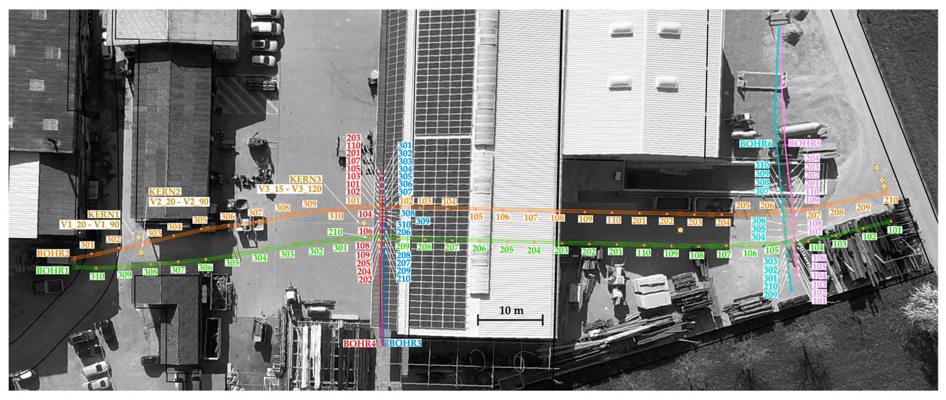
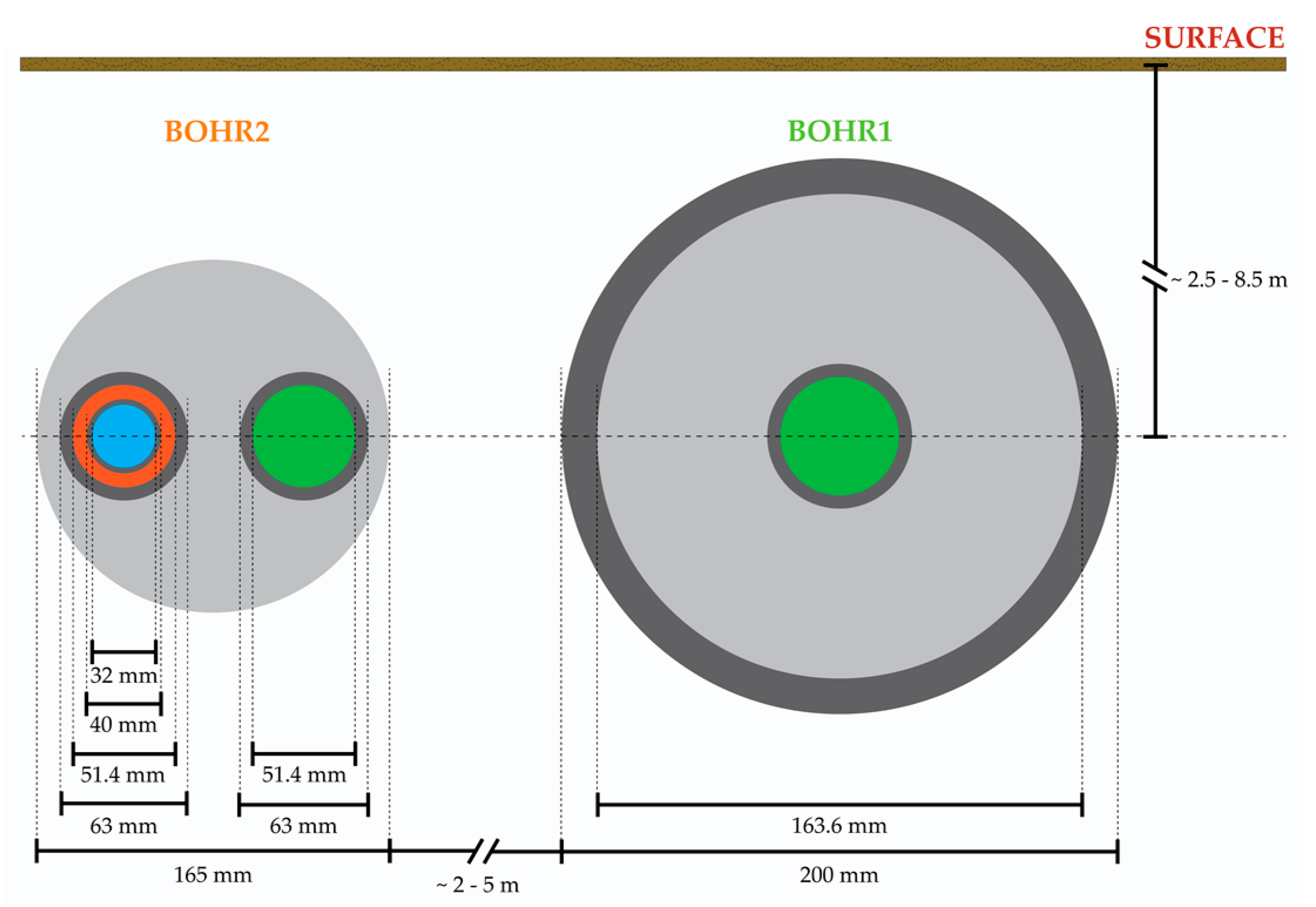
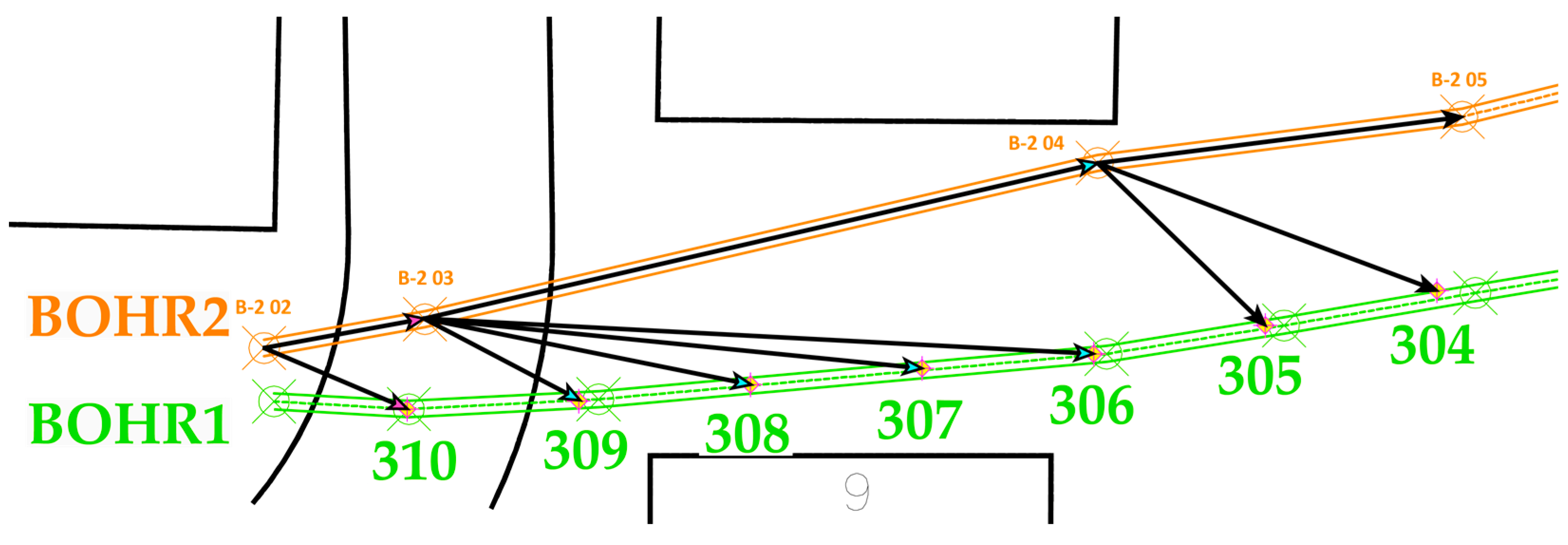
2.2. Experimental Test Site
 ).
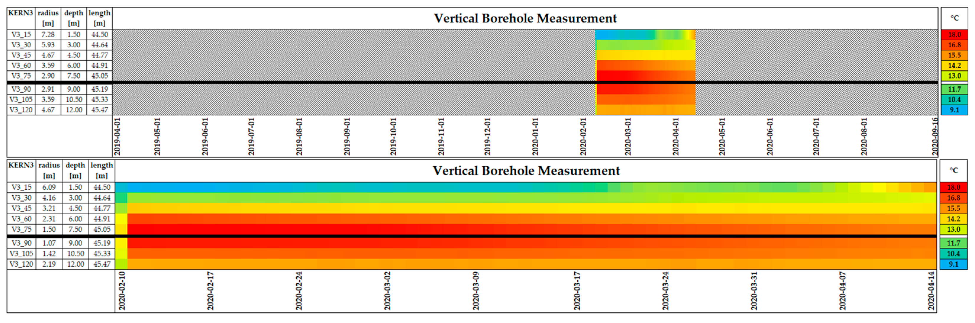
). ). Each of the three vertical boreholes used for measurement had 8 temperature sensors spaced ~1 and ~1.5 m apart. All temperature sensors were recorded with an Agilent 34410A/11A multimeter. The material properties of components used in the construction of the heated borehole and measurement network are listed in Table 3.
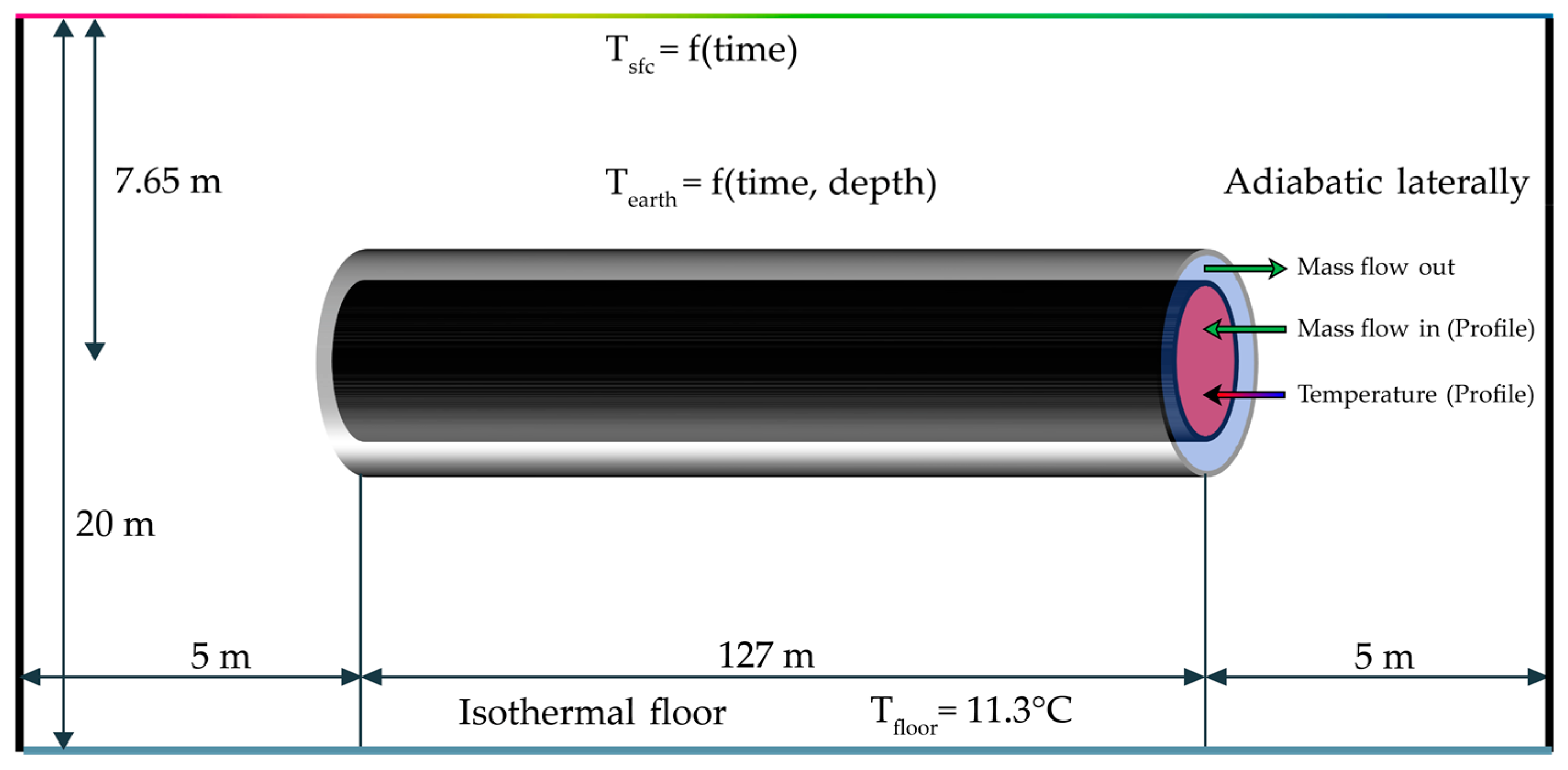
2.3. Modeling a BTES System
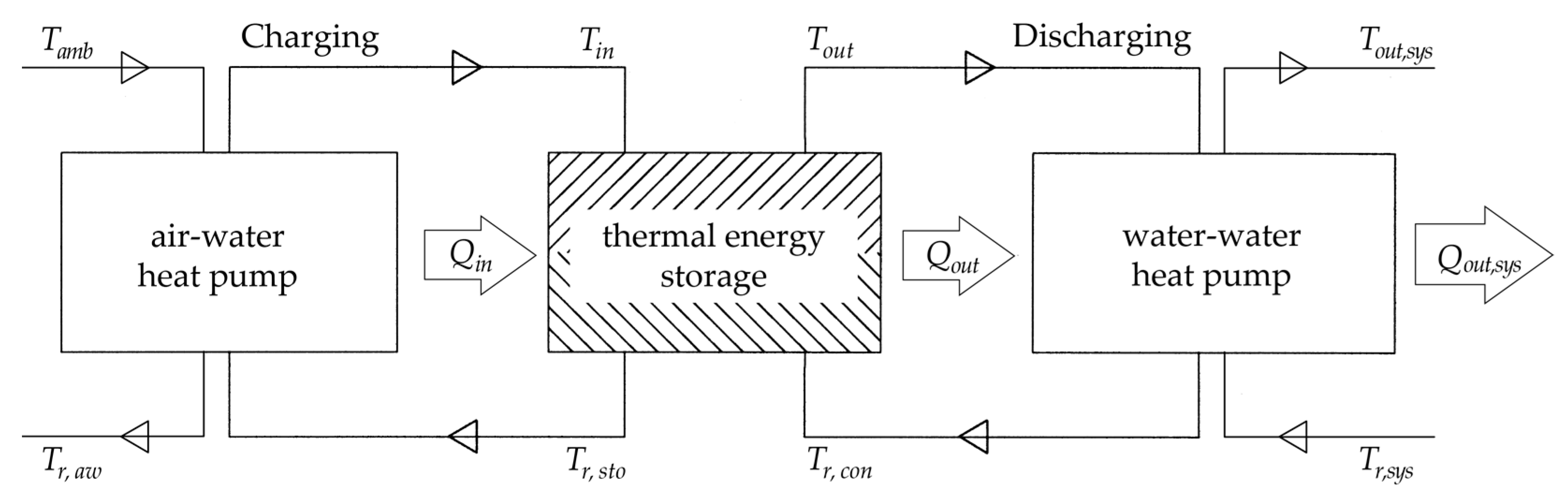
2.4. BTES System
- the difference between the ambient temperature and storage temperature
- the difference between the return temperature from the heat sink and
- the minimum and maximum outlet temperatures for a heat and cold storage, respectively
- the quantity of stored thermal energy
- the installed depth of the storage system
- the ratio between the length and cross-sectional width of the energy storage system
- the thermal properties of the underground, e.g., groundwater, permeability, anisotropic properties of different soil layers, belowground infrastructure, surface covering, etc.
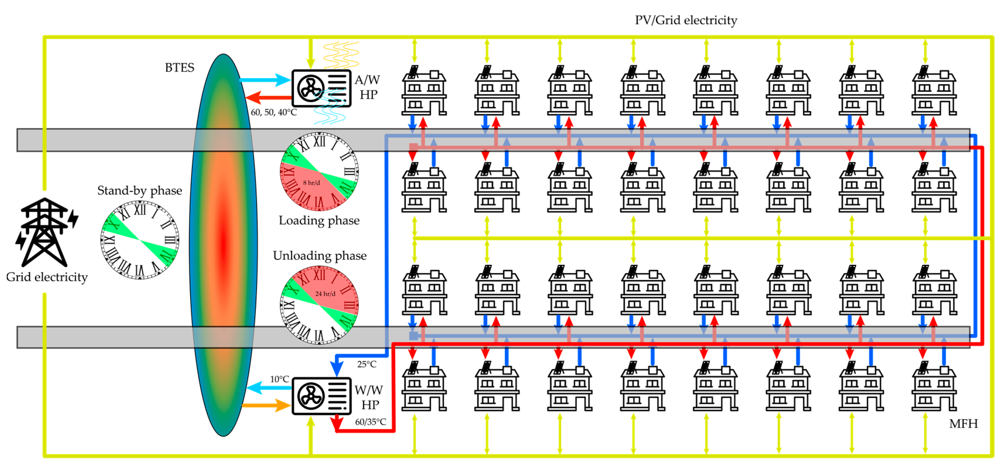
2.4.1. BTES System with a DHN
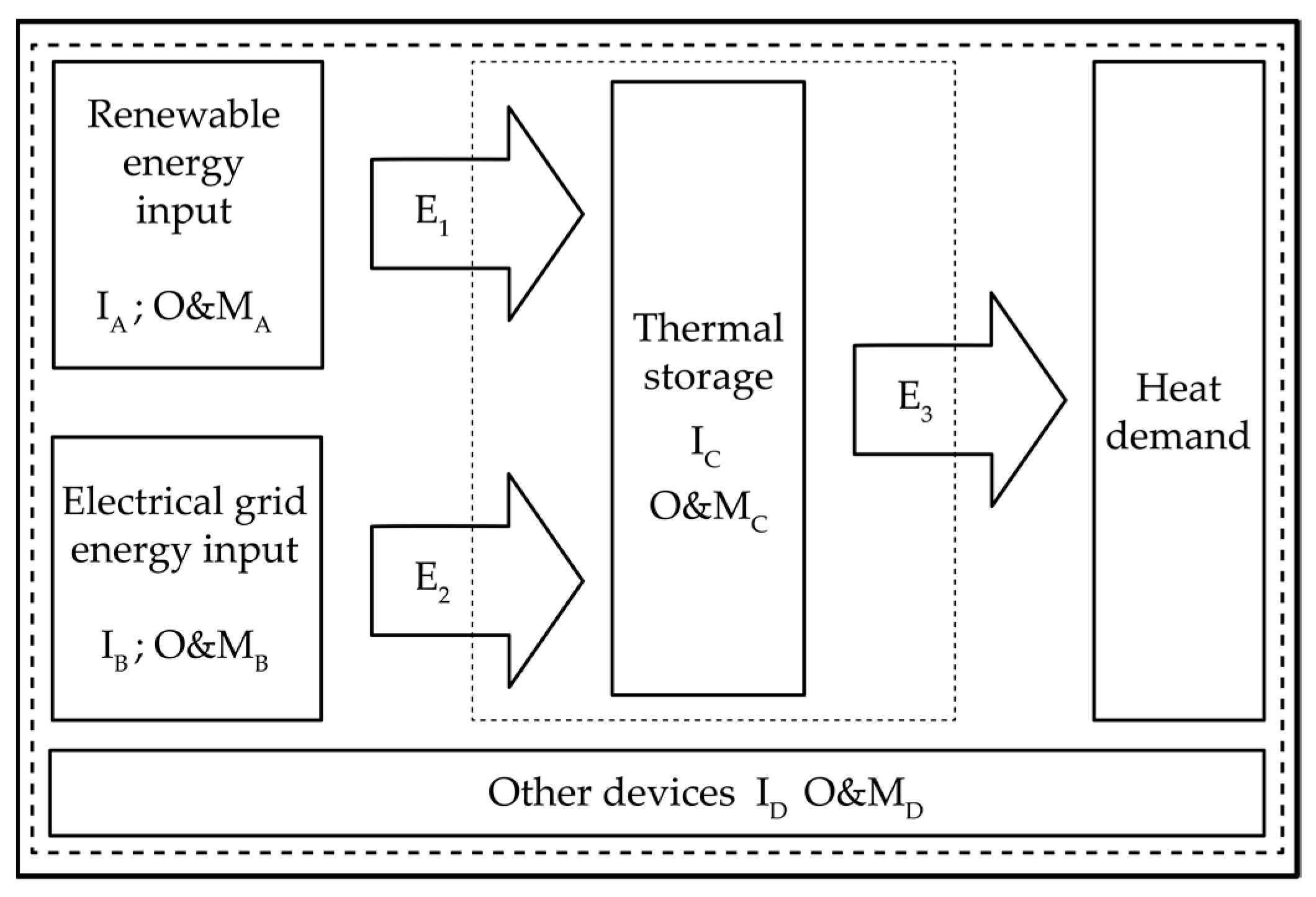
2.5. BTES/DHN Equipment, Investment, and Operating and Maintenance Costs
2.5.1. Electrical Energy Costs
2.5.2. Borehole Costs
2.5.3. Heat Pump Costs
2.5.4. Hydraulic Pump Costs
2.5.5. DHN Costs
3. Results
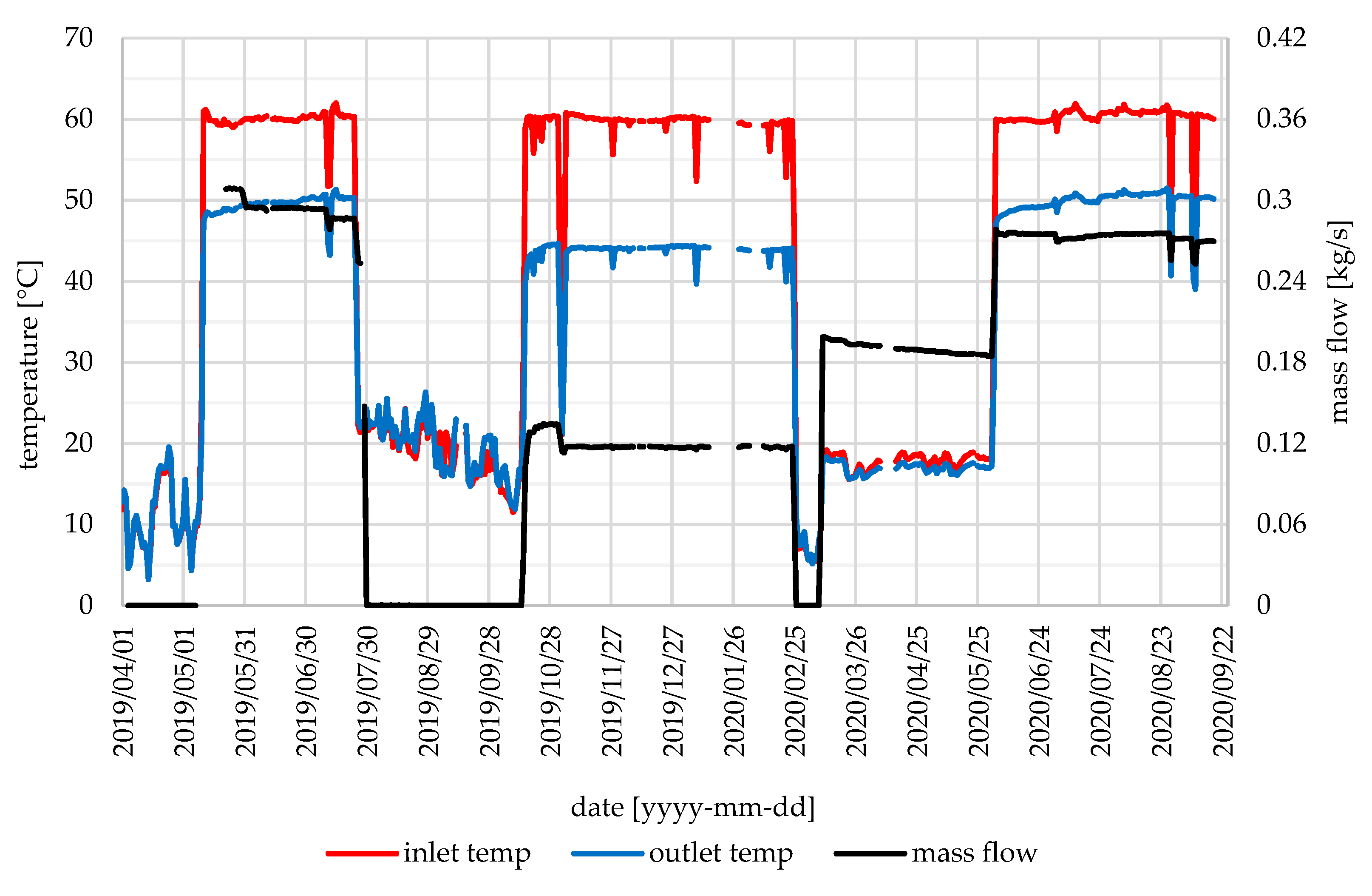
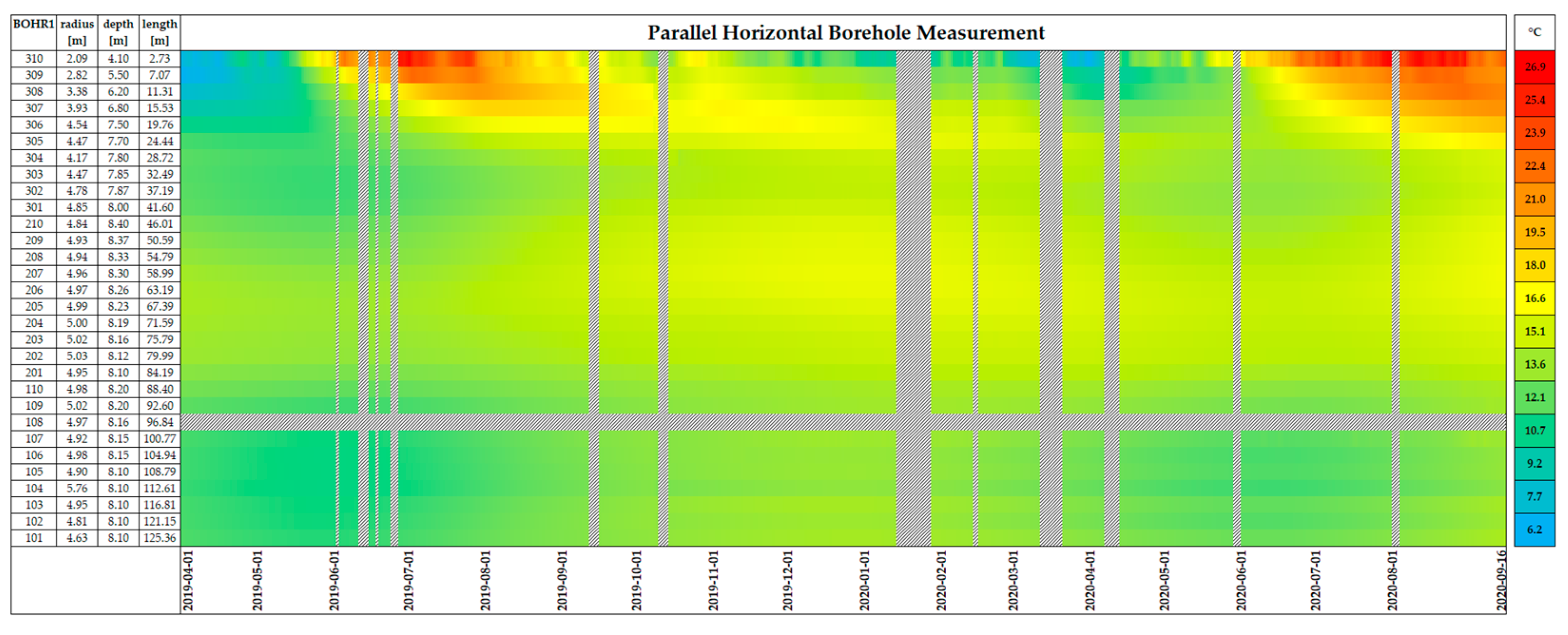
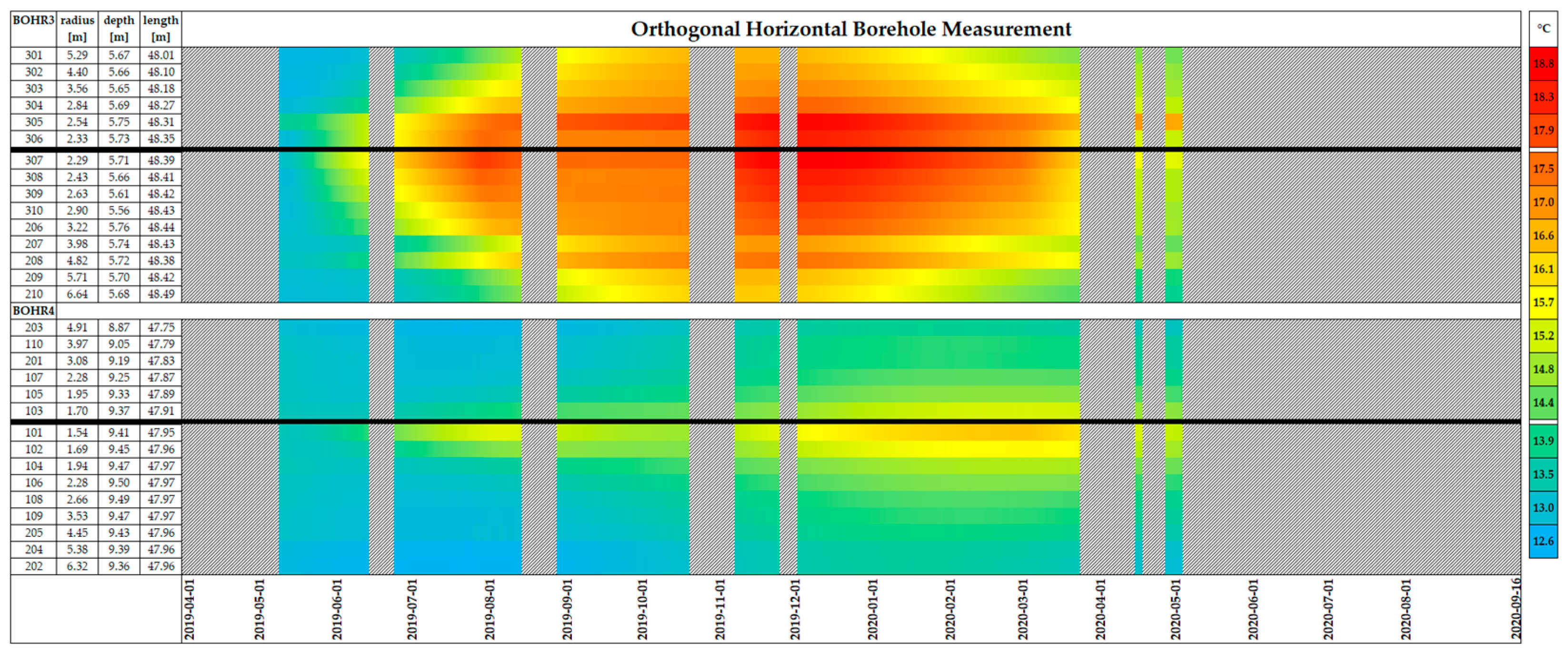
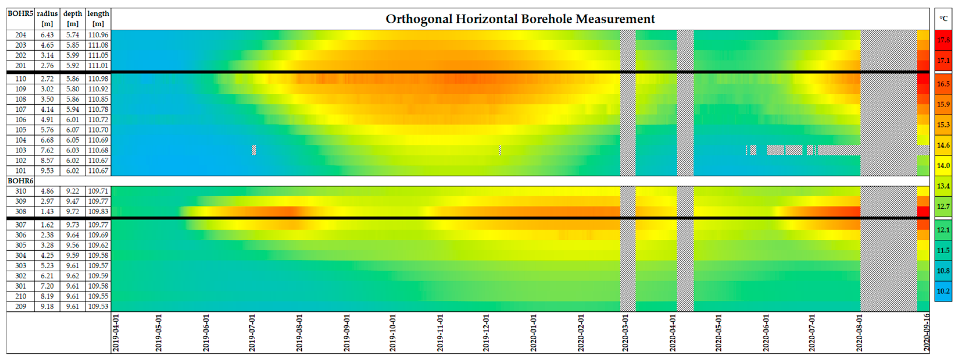
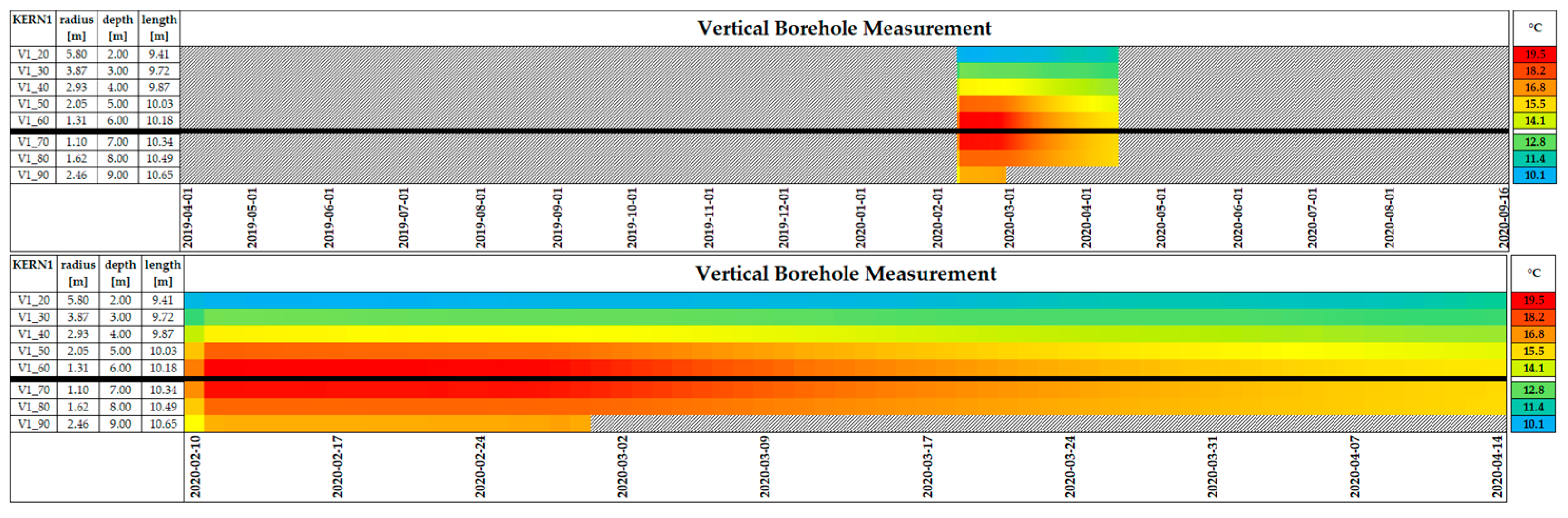
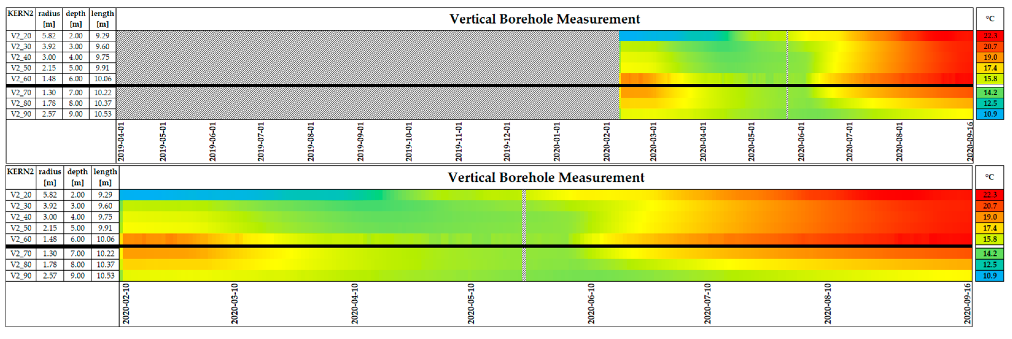
3.1. Experimental Results
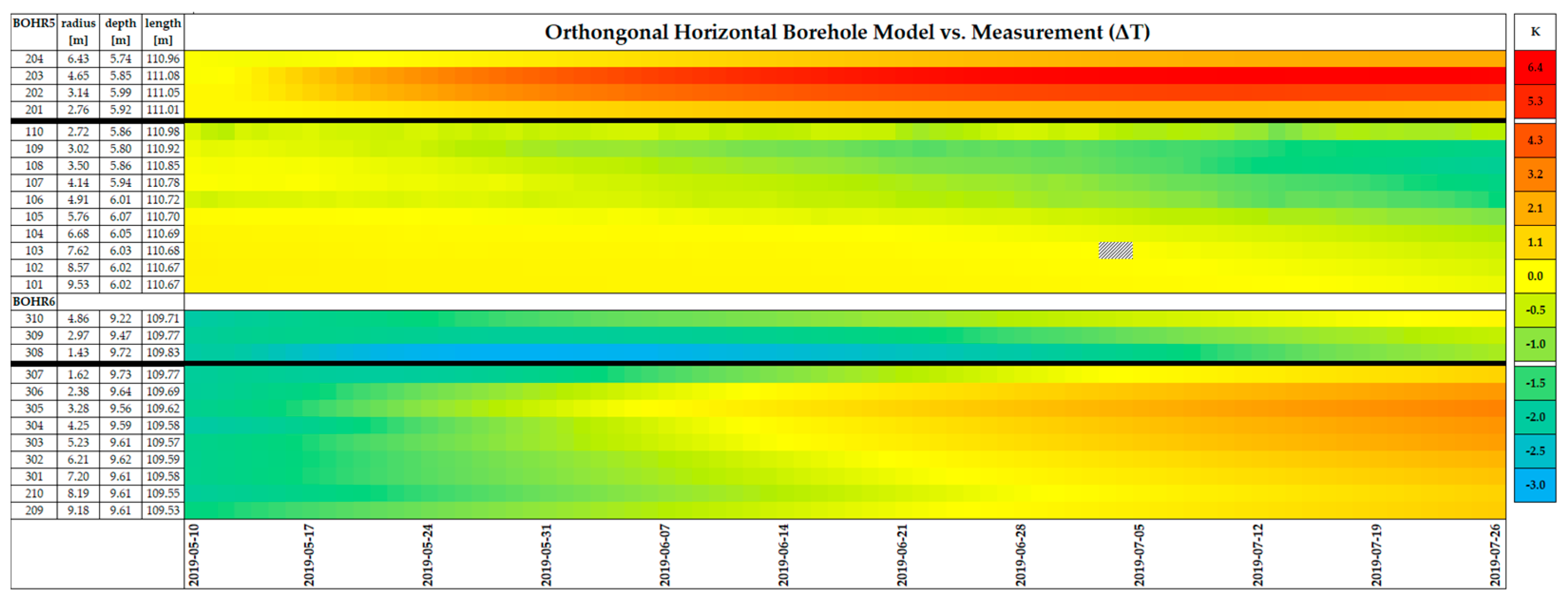
3.2. Model Validation
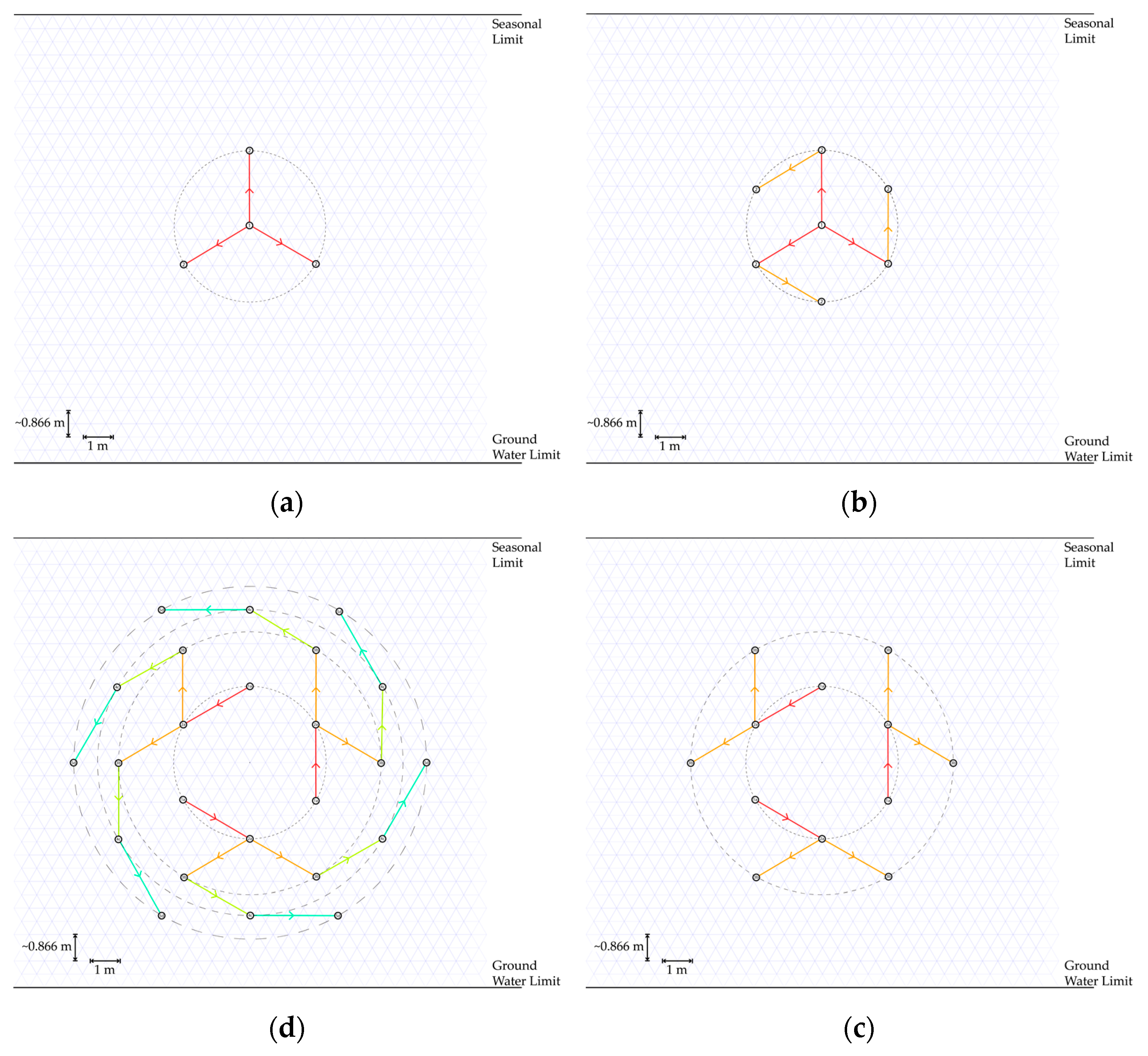
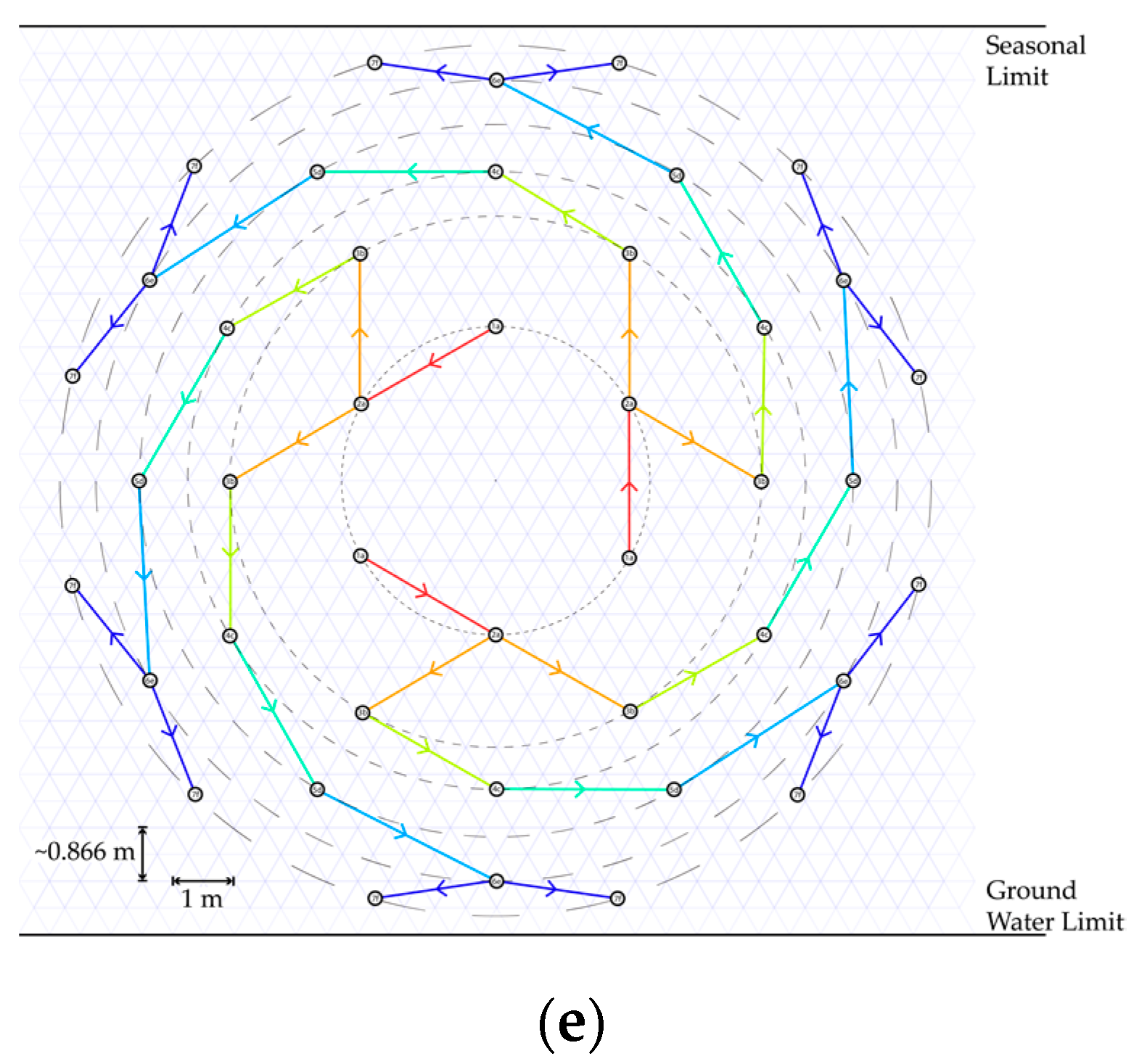
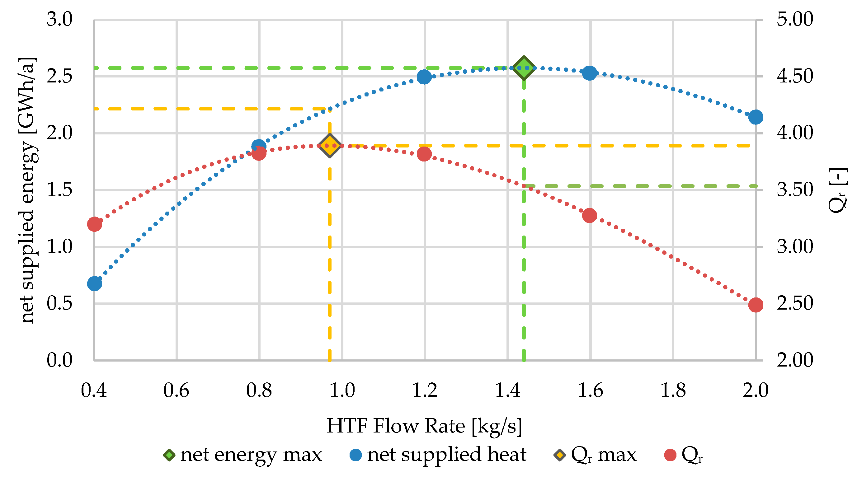
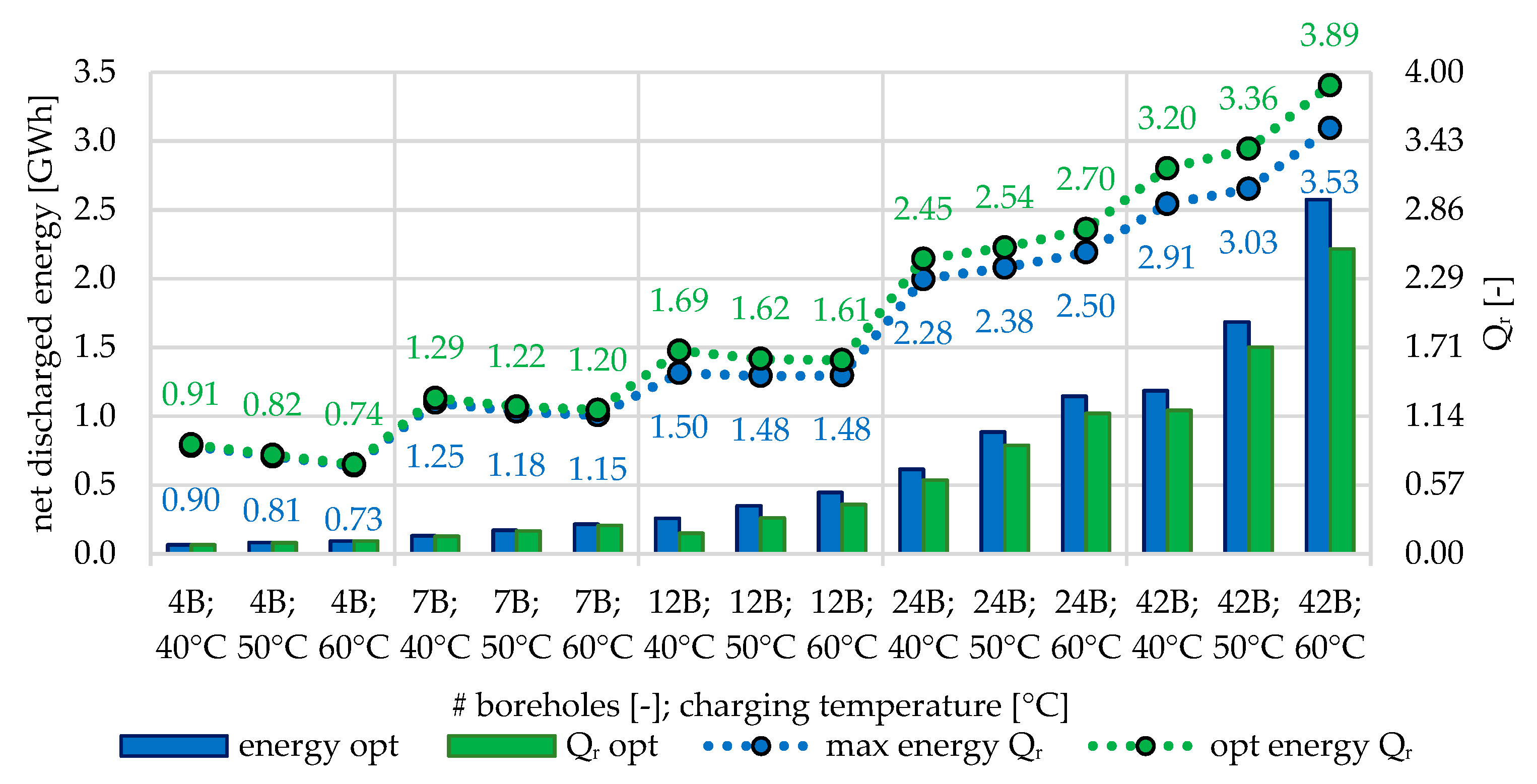
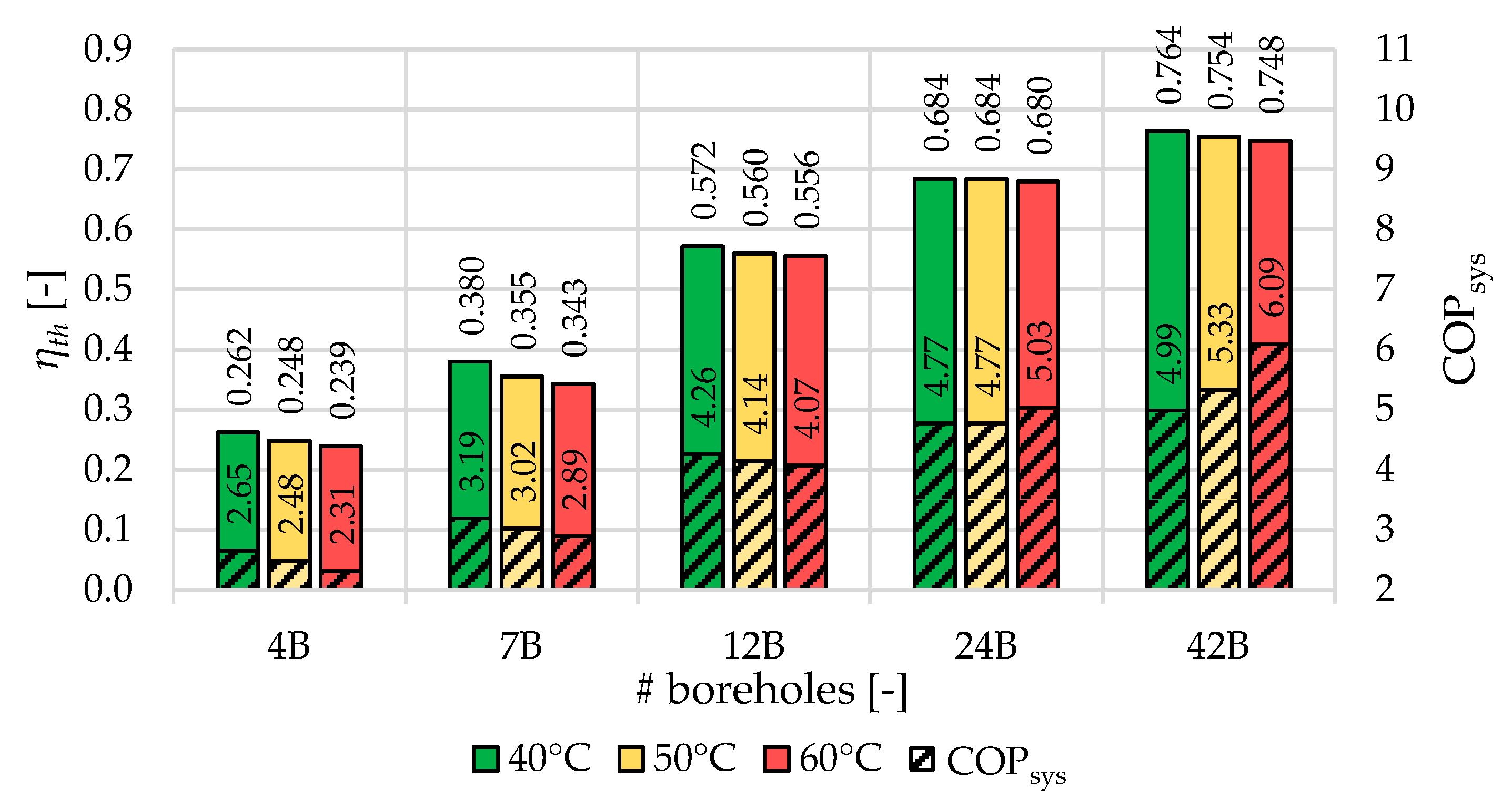
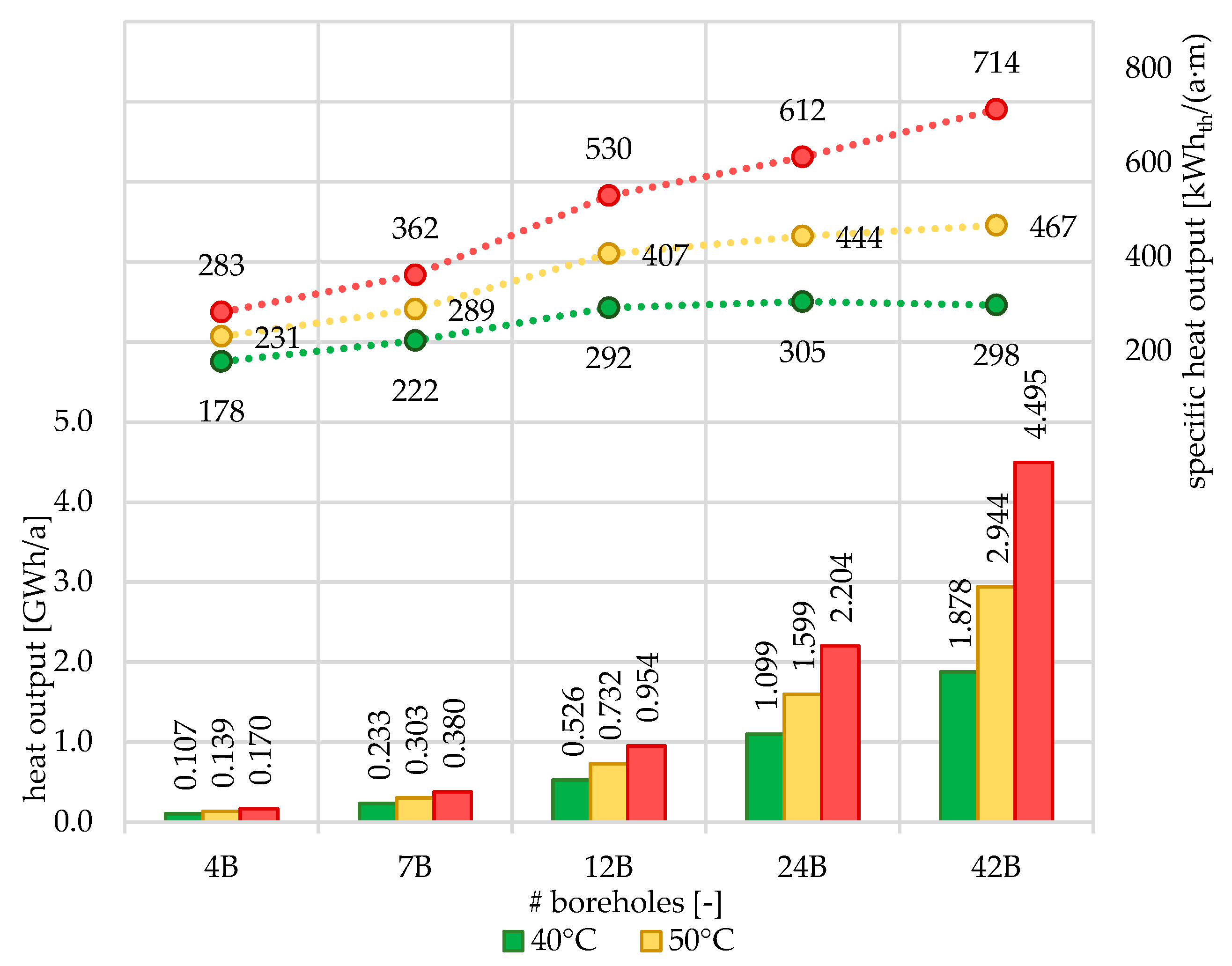
3.3. Multi-Borehole Configurations
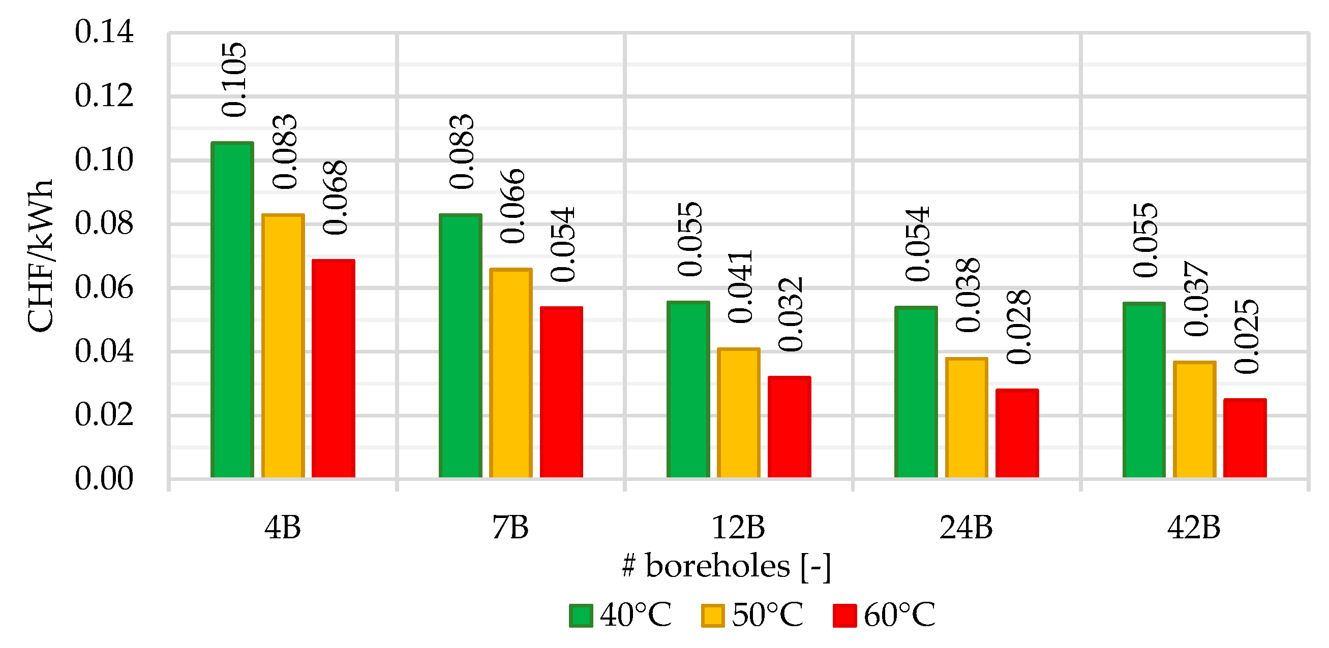
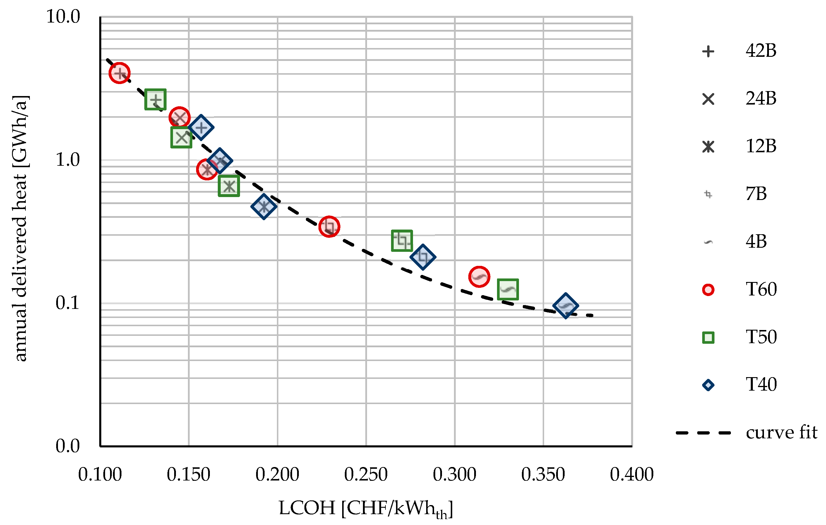
3.4. Economic Evaluation
4. Discussion
4.1. Experimental Results
4.2. Model Output and Economic Analysis
5. Conclusions
Author Contributions
Funding
Data Availability Statement
Conflicts of Interest
Nomenclature
| Term | Definition | Unit |
| 3D-HDD | 3-dimensional horizontally-directed drilling | - |
| AW | air-water heat pump | - |
| BH | building heat | - |
| BOHRX | horizontal borehole X | - |
| BTES | borehole thermal energy storage | - |
| COPi | coefficient of performance of i | - |
| DHN | district heating network | - |
| DHW | domestic hot water | - |
| GPS | global positioning system | - |
| HDPE | high density polyethylene | - |
| HTF | heat transfer fluid | - |
| IEA | International Energy Agency | - |
| IGE | Institute für Gebäudetechnik und Energie; HSLU | - |
| KERNX | vertical borehole X | - |
| MFH | Swiss multi-family house | - |
| Ni | number of component i | - |
| PV | photovoltaic | - |
| SFOE | Swiss Federal Office of Energy | - |
| WW | water-water heat pump | - |
| # | number | - |
| bh | borehole | - |
| calc | calculated | - |
| dhn | district heating network | - |
| el | electric | - |
| hyd | hydraulic | - |
| lat | latitude | - |
| long | longitude | - |
| r | discount rate | - |
| recom | recommended | - |
| th | thermal | - |
| yr | year | - |
| Ai | area of component i | m2 |
| Cp,v | volumetric specific heat capacity | MJ/m3 |
| Ci | cost of component i | CHF/kWh |
| Øi | diameter of component i | m |
| Ei | energy of component i | kWh |
| HD | linear heat demand density | kWh/m |
| Ii | average investment cost of component i | CHF |
| Ii | investment cost of component i | CHF |
| λ | thermal conductivity | W/(m·K) |
| LCOH | levelized cost of heat | CHF/kWhth |
| LCOS | levelized cost of storage | CHF/kWhth |
| Li | length of component i | m |
| O&Mi | operating and maintenance cost of component i | CHF/year |
| Qi | energy quantity of i | kWh |
| ρ | density | kg/m3 |
| spi | spacing between component i | m |
| t | operating years | years |
| XX# | X-X heat pump capacity | kW |
Appendix A

| Term | Equation | Unit | Index |
|---|---|---|---|
| CHF | (1) | ||
| CHF/year | (2) | ||
| . | CHF | (3) | |
| . | CHF | (4) | |
| . | CHF | (5) | |
| . | CHF | (6) | |
| CHF | (7) | ||
| CHF/year | (8) | ||
| CHF | (9) | ||
| CHF/year | (10) | ||
| CHF | (11) | ||
| m | (12) | ||
| CHF | (13) |
| Boreholes Tin | [CHF] | [CHF/yr] | [CHF] | [CHF/yr] | [CHF] | [CHF/yr] | [CHF] | [CHF/yr] |
|---|---|---|---|---|---|---|---|---|
| 4 @ 40 °C | 135,000 | 3896 | 120,731 | 32,847 | 49,123 | 103,226 | 40,775 | 245 |
| 4 @ 50 °C | 135,000 | 4133 | 140,311 | 33,043 | 55,706 | 103,292 | 51,991 | 319 |
| 4 @ 60 °C | 135,000 | 4262 | 159,930 | 33,239 | 61,788 | 103,353 | 64,860 | 390 |
| 7 @ 40 °C | 234,000 | 6564 | 139,947 | 33,039 | 73,576 | 103,471 | 88,969 | 536 |
| 7 @ 50 °C | 234,000 | 7171 | 167,811 | 33,318 | 85,739 | 103,592 | 114,983 | 696 |
| 7 @ 60 °C | 234,000 | 7643 | 196,622 | 33,606 | 98,368 | 103,719 | 144,599 | 872 |
| 12 @ 40 °C | 399,000 | 7354 | 172,139 | 33,361 | 121,027 | 103,945 | 200,210 | 1208 |
| 12 @ 50 °C | 399,000 | 8081 | 214,565 | 33,785 | 150,903 | 104,244 | 278,127 | 1681 |
| 12 @ 60 °C | 399,000 | 8533 | 256,379 | 34,203 | 181,206 | 104,547 | 361,643 | 2190 |
| 24 @ 40 °C | 795,000 | 15,660 | 217,936 | 33,819 | 200,223 | 104,737 | 417,209 | 2523 |
| 24 @ 50 °C | 795,000 | 17,033 | 278,536 | 34,425 | 262,728 | 105,362 | 606,402 | 3670 |
| 24 @ 60 °C | 795,000 | 17,870 | 345,930 | 35,099 | 333,846 | 106,073 | 834,604 | 5058 |
| 42 @ 40 °C | 1,389,000 | 27,464 | 257,174 | 34,211 | 296,038 | 105,695 | 712,115 | 4310 |
| 42 @ 50 °C | 1,389,000 | 32,031 | 355,584 | 35,196 | 416,608 | 106,901 | 1,116,367 | 6756 |
| 42 @ 60 °C | 1,389,000 | 35,326 | 468,221 | 36,322 | 580,494 | 108,540 | 1,702,572 | 10,316 |
References
- Sass, I.; Brehm, D.; Coldewey, W.G.; Dietrich, J.; Klein, R.; Kellner, T.; Kirschbaum, B.; Lehr, C.; Marek, A.; Mielke, P.; et al. Shallow Geothermal Systems—Recommendations on Design, Construction, Operation and Monitoring; Wiley: Hoboken, NJ, USA, 2016; ISBN 9783433031407. [Google Scholar]
- Stevens, V.; Craven, C.; Grunau, B. Thermal Storage Technology Assessment. Rapp. CCHRC 2013, 1, 1–54. [Google Scholar]
- Schmidt, T.; Müller-Steinhagen, H. The Central Solar Heating Plant with Aquifer Thermal Energy Store in Rostock-Results after four years of operation. EuroSun 2004, 1, 20–23. [Google Scholar]
- Reuss, M.; Beuth, W.; Schmidt, M.; Schoelkopf, W. Schoelkopf, Solar District Heating with Seasonal Storage in Attenkirchen. In Proceedings of the IEA Conf. ECOSTOCK, Richard Stock. Coll., Pomona, NJ, USA, May 31–2 June 2006. [Google Scholar]
- Nussbicker, J.; Mangold, D.; Heidemann, W.; Muller-Stenhagen, H. Solar Assisted District Heating System with Duct Heat Store in Neckarsulm-Amorbach (Germany). ISES Sol. World Congr. 2003, 2003, 1–6. [Google Scholar]
- Mangold, D.; Schmidt, T.; Müller-Steinhagen, H. Seasonal thermal energy storage in Germany. Struct. Eng. Int. J. Int. Assoc. Bridg. Struct. Eng. 2004, 14, 230–232. [Google Scholar] [CrossRef]
- Persson, J.; Westermark, M. Low-energy buildings and seasonal thermal energy storages from a behavioral economics perspective. Appl. Energy 2013, 112, 975–980. [Google Scholar] [CrossRef]
- Wong, B.; Mesquita, L. Drake landing solar community: Financial summary and lessons learned. In Proceedings of the ISES Solar World Congress 2019/IEA SHC International Conference on Solar Heating and Cooling for Buildings and Industry, Santiago, Chile, 4–9 November 2019; pp. 482–493. [Google Scholar]
- Fisch, M.N.; Guigas, M.; Dalenbäck, J.O. A review of large-scale solar heating system in Europe. Solar Energy 1998, 63, 355–366. [Google Scholar] [CrossRef]
- Sibbitt, B.; McClenahan, D.; Djebbar, R.; Thornton, J.; Wong, B.; Carriere, J.; Kokko, J. The performance of a high solar fraction seasonal storage district heating system-Five years of operation. Energy Procedia 2012, 30, 856–865. [Google Scholar] [CrossRef]
- Mangold, D. Seasonal storage—A German success story. Sun Wind Energy 2007, 1, 48–59. [Google Scholar]
- Der Schweizerische Bundesrat, Gewässerschutzverordnung SR 814.201 (GSchV) vom 28. Oktober 1998 (Stand am 1 January 2018), n.d. Available online: https://www.admin.ch/opc/de/classified-compilation/19983281/index.html (accessed on 20 January 2022).
- VDI-Gesellschaft Verfahrenstechnik und Chemieingenieurwesen. VDI 4640 Blatt 3; Thermische Nutzung des Untergrundes, Unterirdische Thermische Energiespeicher; VDI-Gesellschaft Verfahrenstechnik und Chemieingenieurwesen: Düsseldorf, Germany, 2001. [Google Scholar]
- Skarphagen, H.; Banks, D.; Frengstad, B.S.; Gether, H. Design Considerations for Borehole Thermal Energy Storage (BTES): A Review with Emphasis on Convective Heat Transfer. Geofluids 2019, 2019, 1–26. [Google Scholar] [CrossRef]
- Mesquita, L.; McClenahan, D.; Thornton, J.; Carriere, J.; Wong, B. Drake Landing solar community: 10 years of operation. In Proceedings of the ISES Solar World Conference 2017 and the IEA SHC Solar Heating and Cooling Conference for Buildings and Industry, AbuDhabi, United Arab Emirates, 29 October–2 November 2017; pp. 333–344. [Google Scholar]
- COMSOL. COMSOL Multiphysics®. 2022. Available online: https://doc.comsol.com/6.0/docserver/#!/com.comsol.help.comsol/helpdesk/helpdesk.html (accessed on 20 July 2022).
- Beaufait, R.; Ammann, S.; Fischer, L. The elephant problem—determining bulk thermal diffusivity. Energies 2021, 14, 7444. [Google Scholar] [CrossRef]
- SIA. Erdwärmesonden SIA 384/6; SIA: Luzern, Switzerland, 2010. [Google Scholar]
- Márquez, J.M.A.; Bohórquez, M.Á.M.; Melgar, S.G. Ground thermal diffusivity calculation by direct soil temperature measurement. application to very low enthalpy geothermal energy systems. Sensors 2016, 16, 306. [Google Scholar] [CrossRef] [PubMed]
- Tavman, I.; Aydogdu, Y.; Kök, M.; Turgut, A.; Ezan, A. Measurement of heat capacity and thermal conductivity of HDPE/expanded graphite nanocomposites by differential scanning calorimetry. Arch. Mater. Sci. Eng. 2011, 50, 56–60. [Google Scholar]
- Erdw, F. GEROtherm ® Technisches Datenblatt GEROtherm ®-Flux Erdwärmesonde, (n.d.). Available online: www.hakagerodur.ch (accessed on 20 July 2022).
- Plötze, M.; Schärli, U.; Weber, H. Thermophysical Properties of Bentonite. In Thermal Processes in Welding; Springer: Berlin/Heidelberg, Germany, 2019; pp. 41–54. [Google Scholar] [CrossRef]
- Kind, M.; Martin, H. Verein Deutscher Ingenieure (VDI)-Heat Atlas; Springer: Berlin/Heidelberg, Germany, 2010; ISBN 9783540778769. [Google Scholar]
- Intro-Meteonorm (de). n.d. Available online: https://meteonorm.com/ (accessed on 19 November 2019).
- Lanahan, M.; Tabares-Velasco, P.C. Seasonal thermal-energy storage: A critical review on BTES systems, modeling, and system design for higher system efficiency. Energies 2017, 10, 743. [Google Scholar] [CrossRef]
- Wang, H.; Qi, C. Performance study of underground thermal storage in a solar-ground coupled heat pump system for residential buildings. Energy Build. 2008, 40, 1278–1286. [Google Scholar] [CrossRef]
- McDaniel, B.; Kosanovic, D. Modeling of combined heat and power plant performance with seasonal thermal energy storage. J. Energy Storage 2016, 7, 13–23. [Google Scholar] [CrossRef]
- Villasmil, W.; Troxler, M.; Hendry, R.; Worlitschek, J. OPTSAIS–Exergetic and Economic Optimization of Seasonal Thermal Energy Storage Systems. 2019, pp. 1–65. Available online: https://www.aramis.admin.ch/Default?DocumentID=62816&Load=true (accessed on 23 January 2021).
- SIA 385/2 (2015); Anlagen für Trinkwarmwasser in Gebäuden-Warmwasserbedarf, Gesamtanforderungen und Auslegung. Schweizerischer Ingenieur-und Architektenverein: Zürich, Switzerland, 2014.
- Jordan, U.; Vajen, K. DHWcalc: Tool for the Generation of Domestic Hot Water Profiles on a Statistical Basis (Version 1.10); DHWcal Man. Version 2.02b; University of Kassel: Kassel, Germany, 2017; Volume 10, pp. 1–14. [Google Scholar]
- BFE, Bau- und Wohnungswesen 2017 - Bau- und Wohnbaustatistik 2017, Gebäude- und Wohnungsstatistik 2017, Leerwohnungszählung vom 1. Juni 2018 | Publikation. n.d. Available online: https://www.bfs.admin.ch/bfs/de/home/statistiken/bau-wohnungswesen.assetdetail.7966565.html (accessed on 19 November 2019).
- Kanton Bern. Bauverordnung (BauV). 2017. Available online: https://www.belex.sites.be.ch/frontend/versions/923 (accessed on 1 June 2018).
- Kanton Zürich. Planungs- und Baugesetz (PBG). 2018. Available online: https://www.zh.ch/internet/de/rechtliche_grundlagen/gesetze/erlass.html?Open&Ordnr=700.1 (accessed on 1 June 2018).
- Nussbaumer, T.; Thalmann, S. Status Report on District Heating Systems in IEA Countries. 2014. Available online: www.bfe.admin.ch/forschung/biomasse (accessed on 15 March 2020).
- Chambers, J.; Zuberi, M.J.S.; Streicher, K.N.; Patel, M.K. Geospatial global sensitivity analysis of a heat energy service decarbonisation model of the building stock. Appl. Energy 2021, 302, 117592. [Google Scholar] [CrossRef]
- Rathgeber, C.; Hiebler, S.; Lävemann, E.; Dolado, P.; Lazaro, A.; Gasia, J.; De Gracia, A.; Miró, L.; Cabeza, L.F.; König-Haagen, A.; et al. IEA SHC Task 42 / ECES Annex 29—A simple tool for the economic evaluation of thermal energy storages. In Proceedings of the SHC 2015, International Conference on Solar Heating and Cooling for Buildings and Industry, Istanbul, Turkey, 2–4 December 2015; Volume 91, pp. 197–206. [Google Scholar]
- Yang, T.; Liu, W.; Kramer, G.J.; Sun, Q. Seasonal thermal energy storage: A techno-economic literature review. Renew. Sustain. Energy Rev. 2021, 139, 110732. [Google Scholar] [CrossRef]
- Schweizerische Eidgenossesschaft, Strompreis Schweiz. 2022. Available online: https://www.strompreis.elcom.admin.ch/?period=2021&category=H4&product=standard (accessed on 15 July 2022).
- Schenk, A.G. Richtpreise Horizontalspülbohrungen; Swiss Association of Engineers and Architects: Heldswil, Switzerland, 2020; Volume 1. [Google Scholar]
- Arpagaus, C.; Bertsch, S. Industrial Heat Pumps in Switzerland Application Potentials and Case Studies; Swiss Federal Office of Energy: Berne, Switzerland, 2020; p. 74. Available online: https://www.aramis.admin.ch/Default?DocumentID=66033&Load=true (accessed on 29 June 2021).
- Popovski, E.; Fleiter, T.; Santos, H.; Leal, V.; Fernandes, E.O. Technical and economic feasibility of sustainable heating and cooling supply options in southern European municipalities-A case study for Matosinhos, Portugal. Energy 2018, 153, 311–323. [Google Scholar] [CrossRef]


| Rock/Soil Type | W/(m·K) | MJ/m3 | 103 kg/m3 | ||
|---|---|---|---|---|---|
| Recom | Calc | Recom | Calc | ||
| clay, dry | 0.4–1.0 | 0.6 | 1.5–1.6 | 1.5 | 1.8–2.0 |
| clay, saturated | 0.9–2.3 | 1.4 | 2.0–2.8 | 2.3 | 2.0–2.2 |
| sand, dry | 0.3–0.8 | 0.5 | 1.3–1.6 | 1.4 | 1.8–2.2 |
| sand, saturated | 1.5–4.0 | 2.3 | 2.2–2.8 | 2.4 | 1.9–2.3 |
| gravel/stone, dry | 0.4–0.5 | 0.4 | 1.3–1.6 | 1.4 | 1.8–2.2 |
| gravel/stone, saturated | 1.6–2.0 | 1.7 | 2.2–2.6 | 2.3 | 1.9–2.3 |
| fixed moraine | 1.7–2.4 | 1.8 | 1.5–2.5 | 2.0 | 1.9–2.5 |
| peat | 0.2–0.7 | 0.4 | 0.5–3.8 | 1.6 | 0.5–0.8 |
| Parameter | Description | Unit |
|---|---|---|
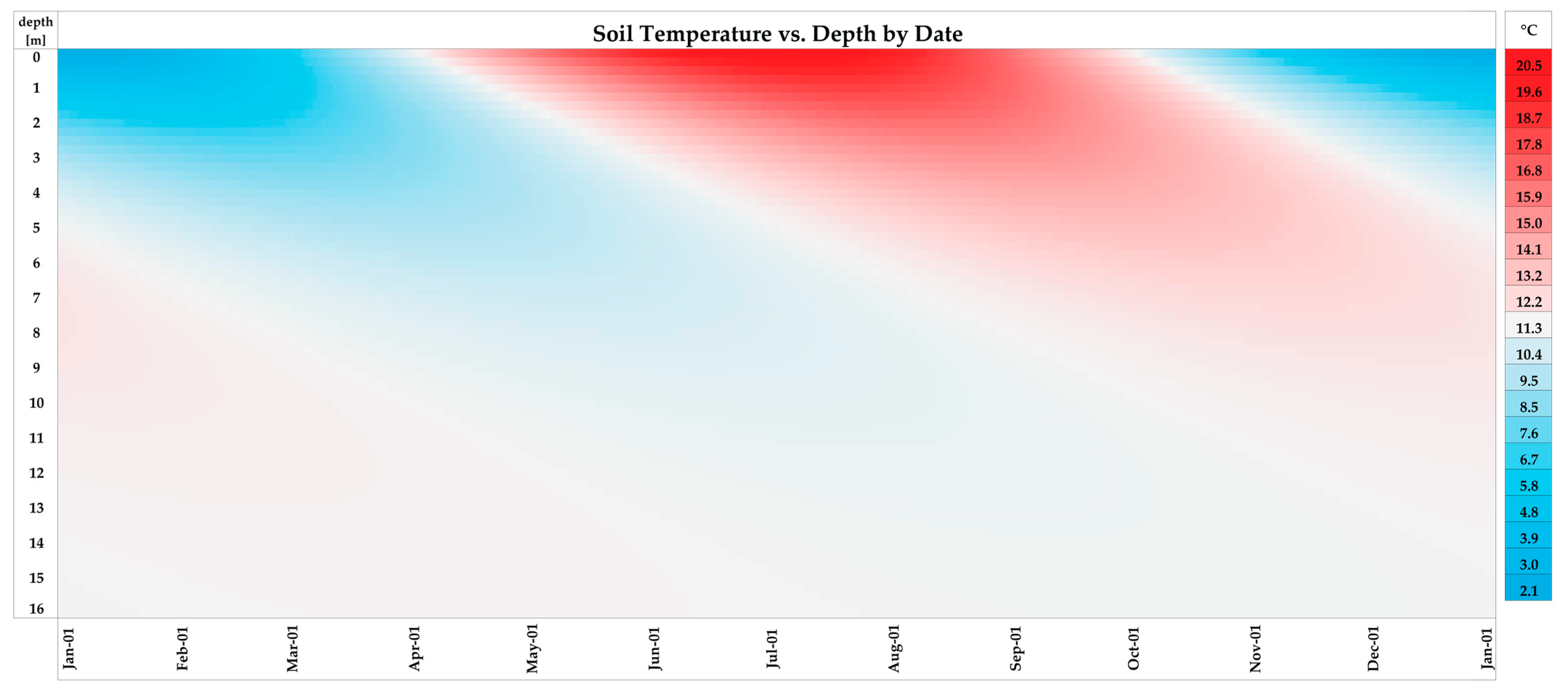
| Soil temperature as a function of depth z and time ts. | K | |
| Initial temperature at a depth z and time ts. | K | |
| Annual amplitude of the monthly average temperature cycle at a given location. | K | |
| Depth under the surface. | m | |
| Thermal diffusivity of soil. | m2/s | |
| Frequency of cycle (1 year). | rad/s | |
| Time elapsed from Jan 1st. | s | |
| Phase shift from Jan 1st for coldest/hottest day of the year. | rad |
| Product | Material | kJ/(kg·K) | W/(m·K) | kg/m3 |
|---|---|---|---|---|
| pipe | HDPE [20,21] | 1.8 | 0.4 | 960 |
| filling material | bentonite [22] | 1.2 | 1.2 | 2000 |
| soil | fixed moraine [18] | 0.9 | 2.0 | 2000 |
| HTF | water * [23] | 4.195–4.183 | 0.58–0.65 | 998–983 |
| Name | Type | Start | End |
|---|---|---|---|
| H1 | heating | 10 May 2019 | 26 July 2019 |
| D1 | drift | 27 July 2019 | 14 October 2019 |
| H2 | heating | 15 October 2019 | 24 February 2020 |
| D2/R1 | drift/recirculation | 25 February 2020 | 1 June 2020 |
| H3 | heating | 2 June 2020 | 18 September 2020 |
| Geology | up to 100 m | 100–200 m | Installation | Location Equip. |
|---|---|---|---|---|
| loose rock | 140 CHF/m | 120 CHF/m | 3000 CHF | 30 CHF/m |
| rock up to 100 MPa | 180 CHF/m | 170 CHF/m | 3000 CHF | 30 CHF/m |
| rock over 100 MPa | 230 CHF/m | 220 CHF/m | 3000 CHF | 30 CHF/m |
Publisher’s Note: MDPI stays neutral with regard to jurisdictional claims in published maps and institutional affiliations. |
© 2022 by the authors. Licensee MDPI, Basel, Switzerland. This article is an open access article distributed under the terms and conditions of the Creative Commons Attribution (CC BY) license (https://creativecommons.org/licenses/by/4.0/).
Share and Cite
Beaufait, R.; Villasmil, W.; Ammann, S.; Fischer, L. Techno-Economic Analysis of a Seasonal Thermal Energy Storage System with 3-Dimensional Horizontally Directed Boreholes. Thermo 2022, 2, 453-481. https://doi.org/10.3390/thermo2040030
Beaufait R, Villasmil W, Ammann S, Fischer L. Techno-Economic Analysis of a Seasonal Thermal Energy Storage System with 3-Dimensional Horizontally Directed Boreholes. Thermo. 2022; 2(4):453-481. https://doi.org/10.3390/thermo2040030
Chicago/Turabian StyleBeaufait, Robert, Willy Villasmil, Sebastian Ammann, and Ludger Fischer. 2022. "Techno-Economic Analysis of a Seasonal Thermal Energy Storage System with 3-Dimensional Horizontally Directed Boreholes" Thermo 2, no. 4: 453-481. https://doi.org/10.3390/thermo2040030