
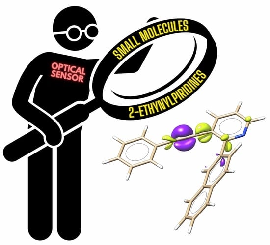
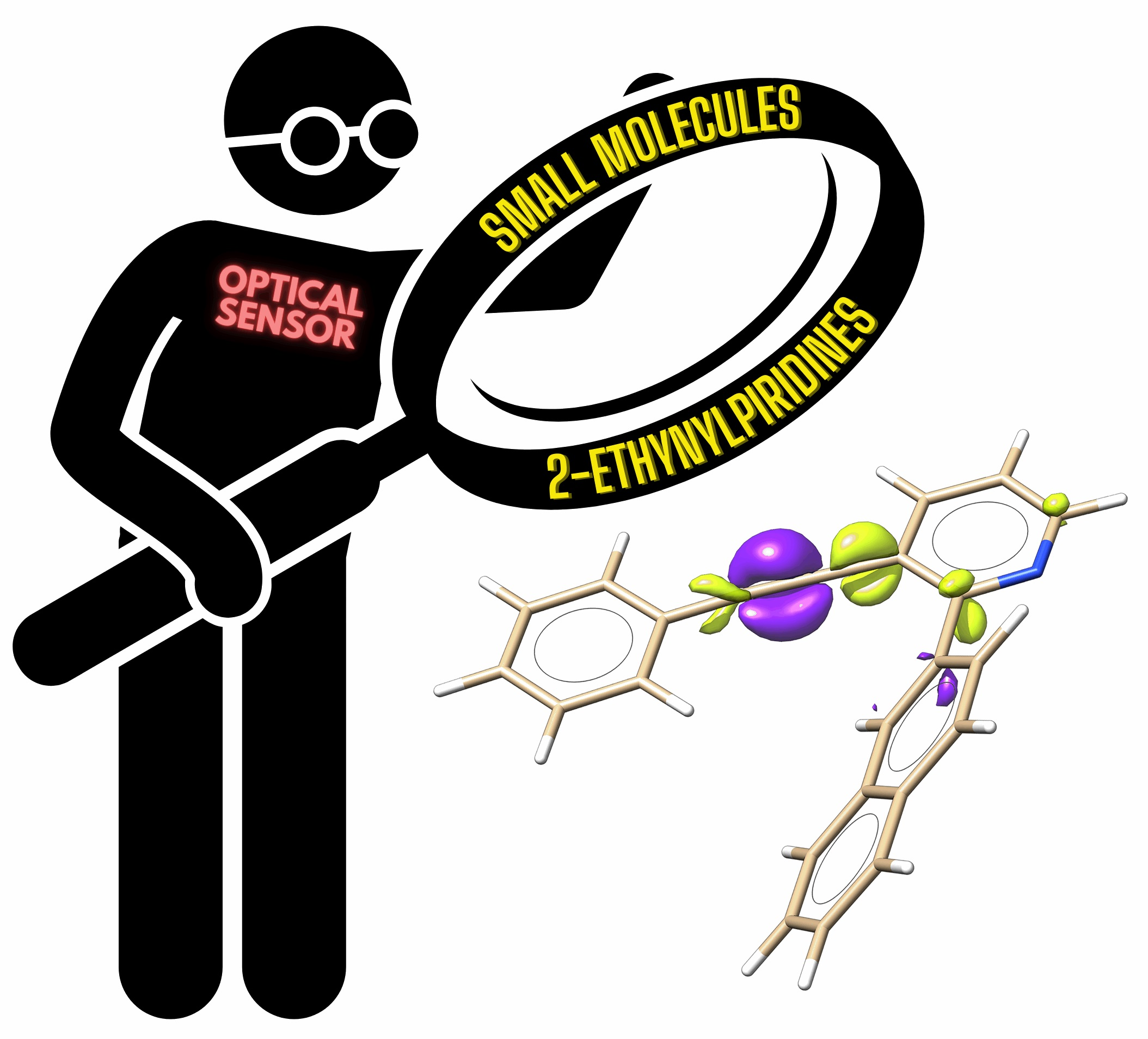
Pyridine-Based Small-Molecule Fluorescent Probes as Optical Sensors for Benzene and Gasoline Adulteration
 , ,
, ,  and
and
Abstract
:
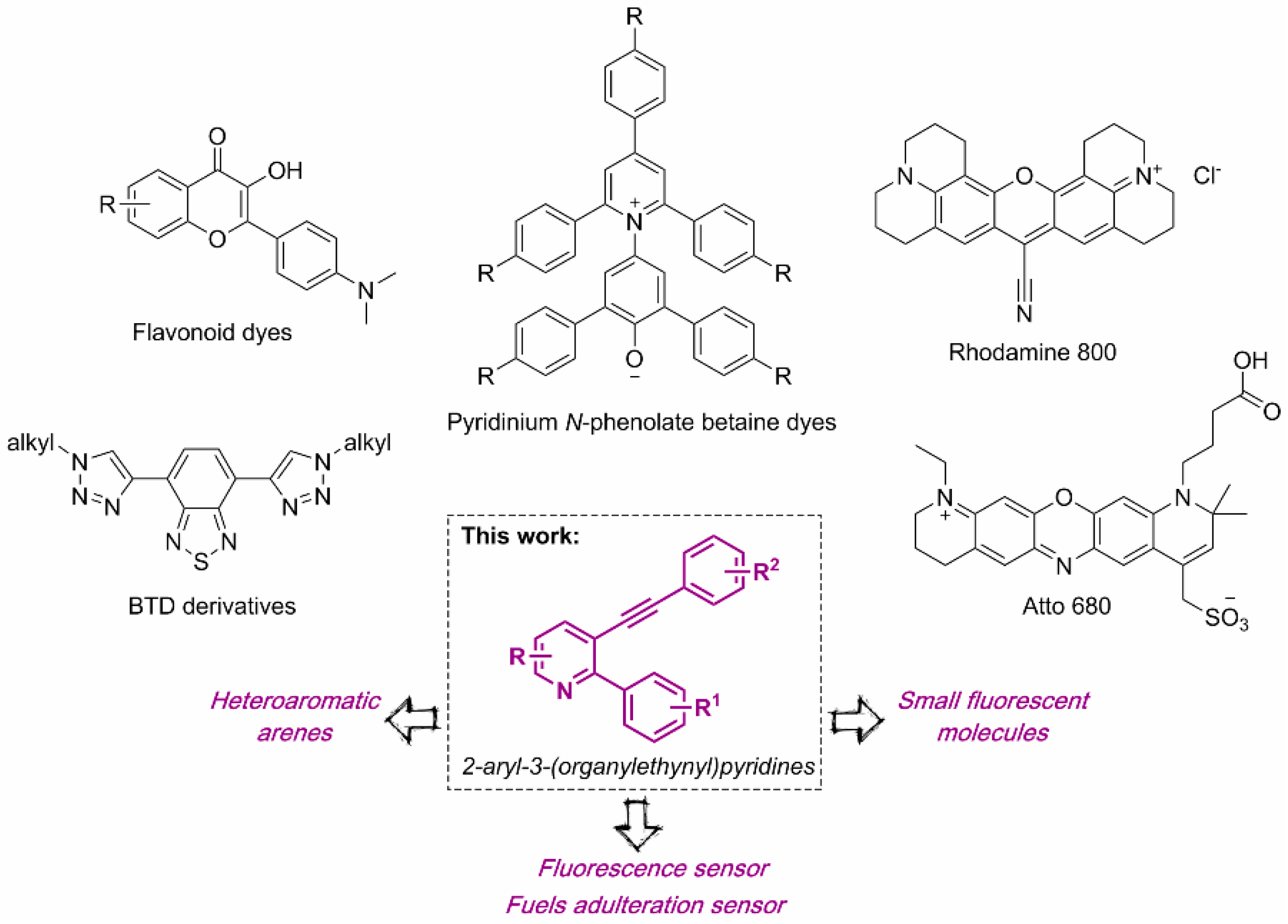
1. Introduction
2. Materials and Methods
2.1. General Information
2.2. Synthesis
2.2.1. General Procedure for the Synthesis of Starting Materials 1a–e
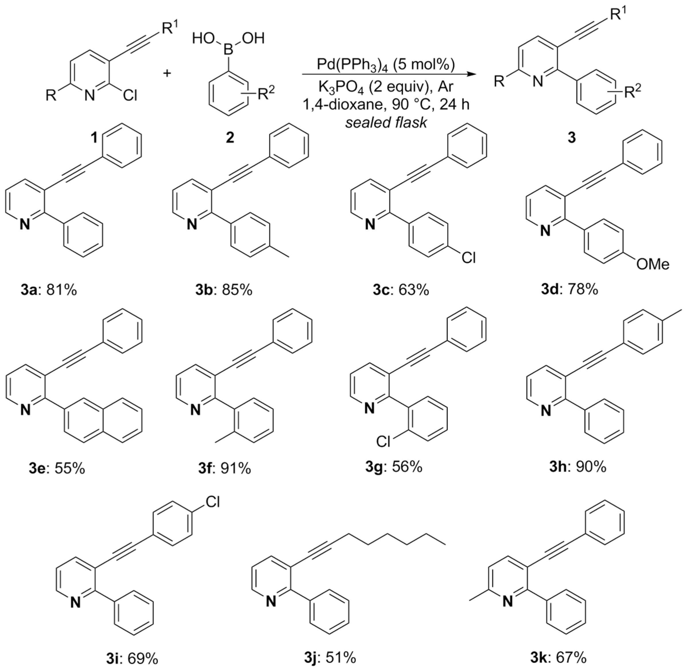
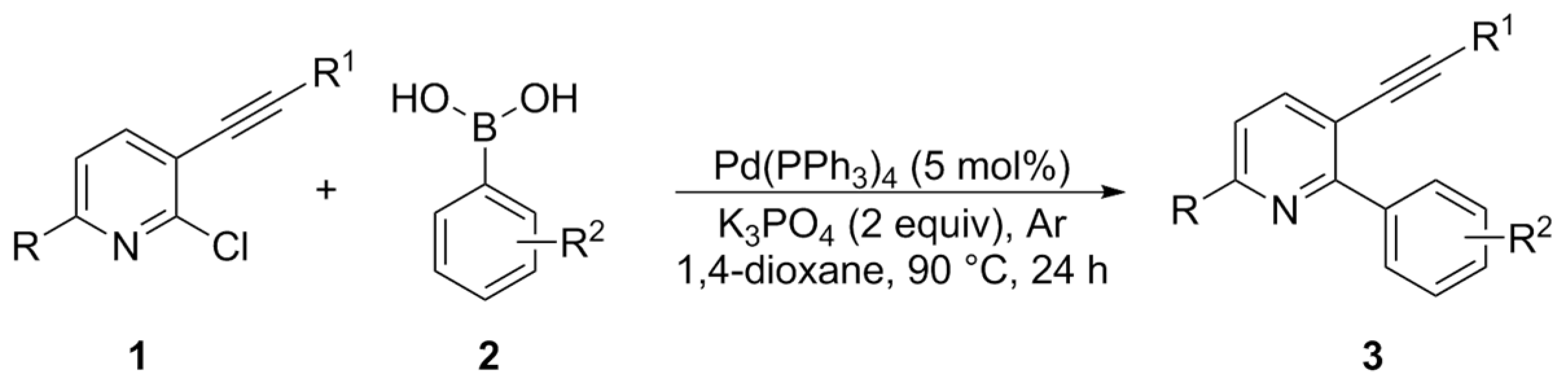
2.2.2. General Procedure for the Synthesis of 2-aryl-3-(organylethynyl)pyridines 3a–k
2.3. Photophysical Characterization
2.4. Fuel Adulteration Sensing
2.5. Theoretical Calculations
3. Results and Discussion
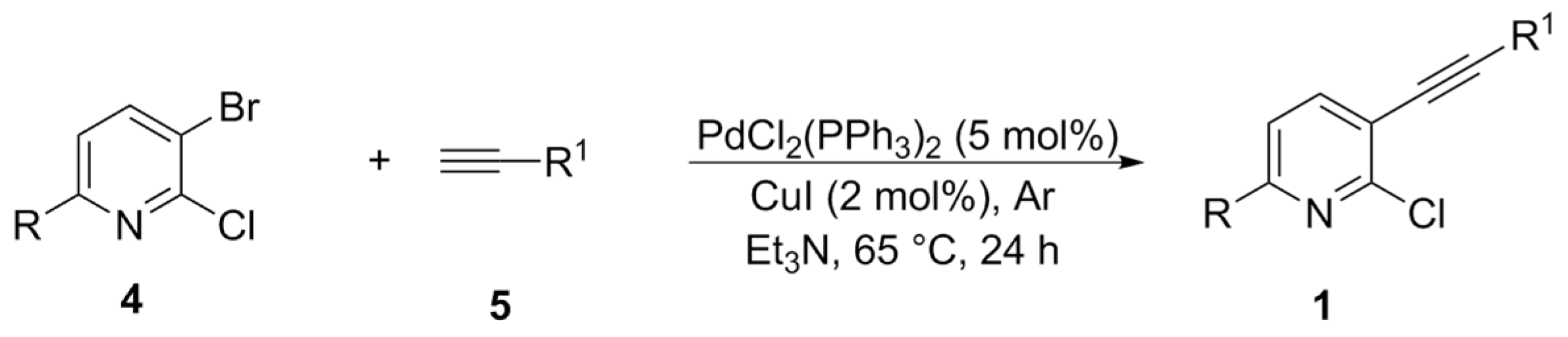
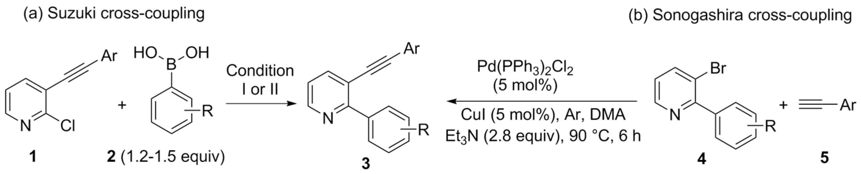
3.1. Synthesis
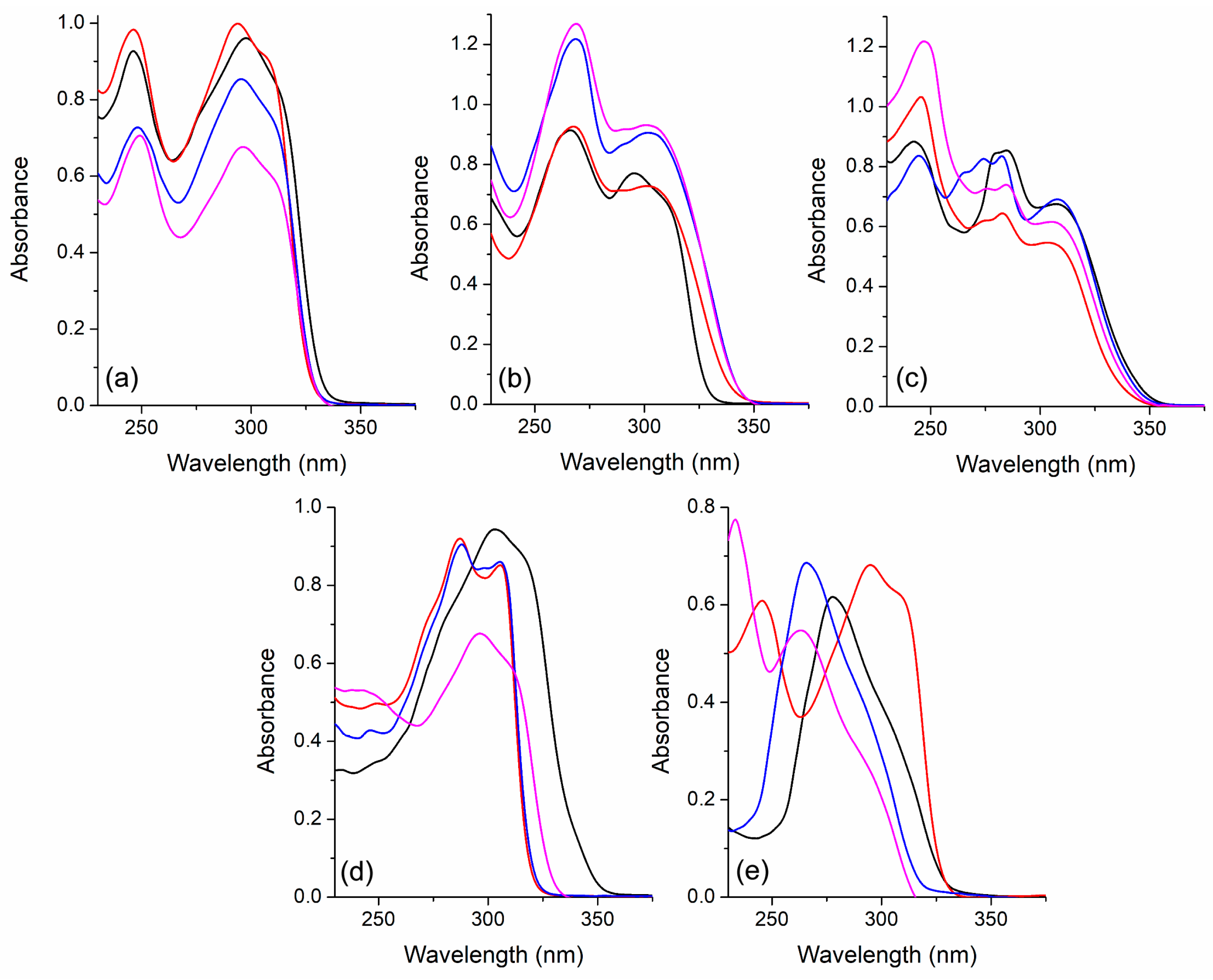
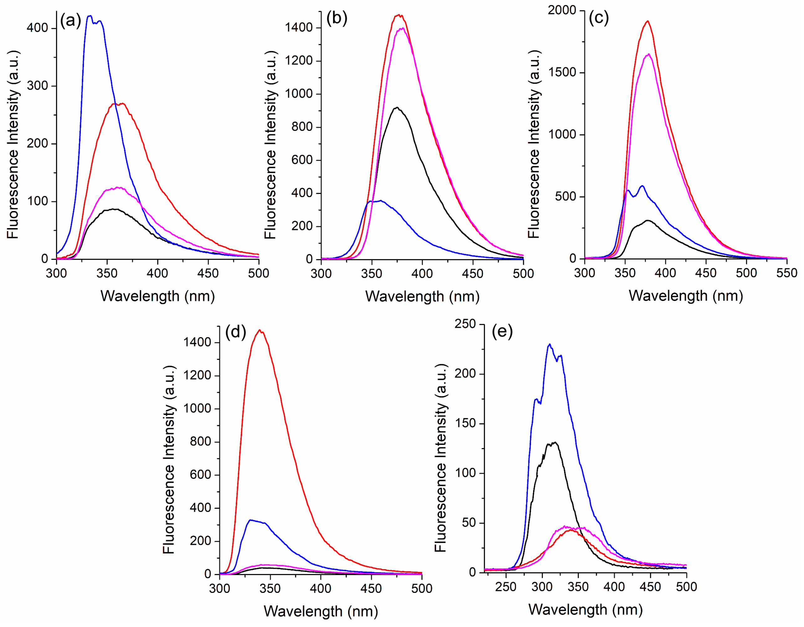
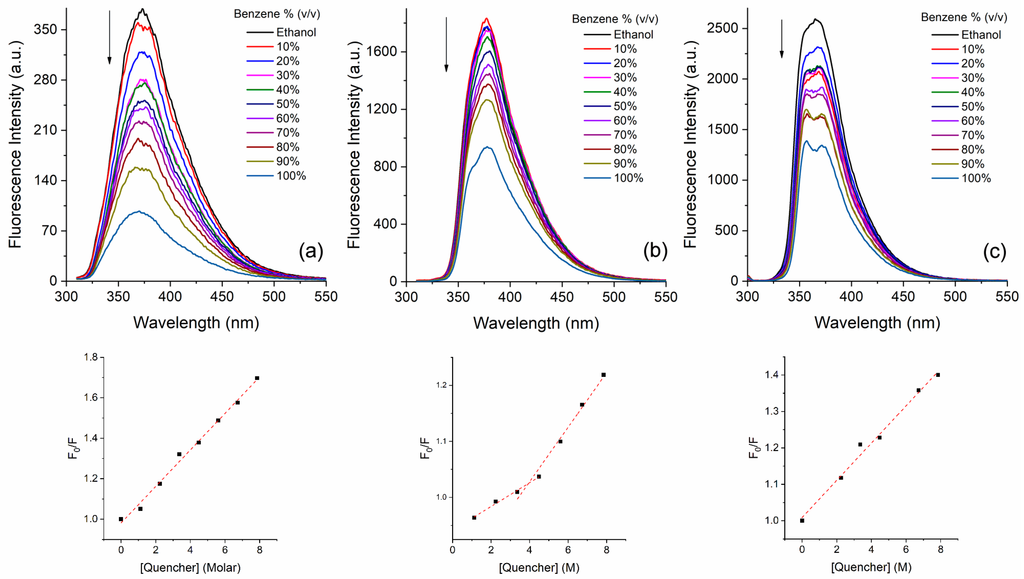
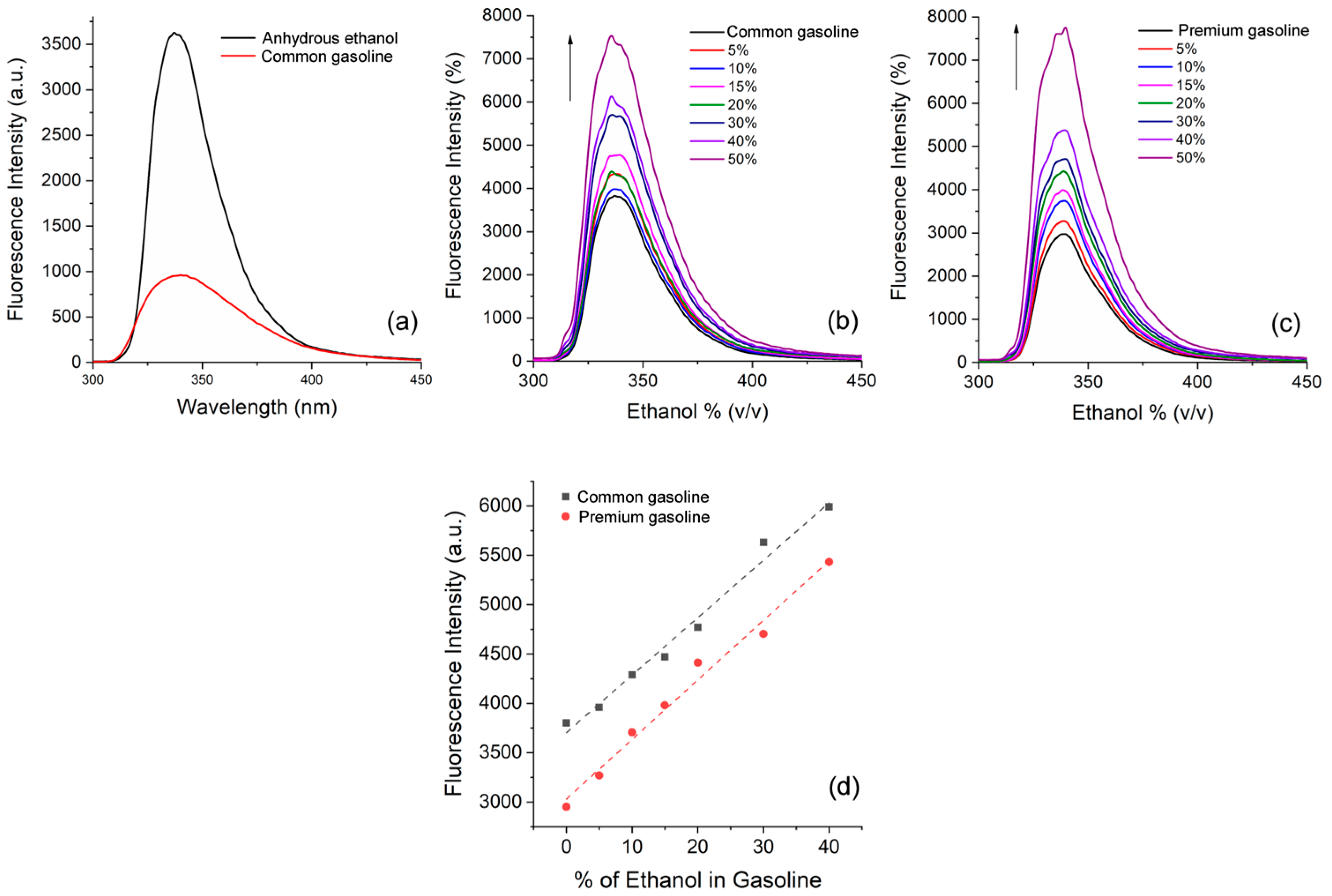
3.2. Photophysics and Optical Sensing
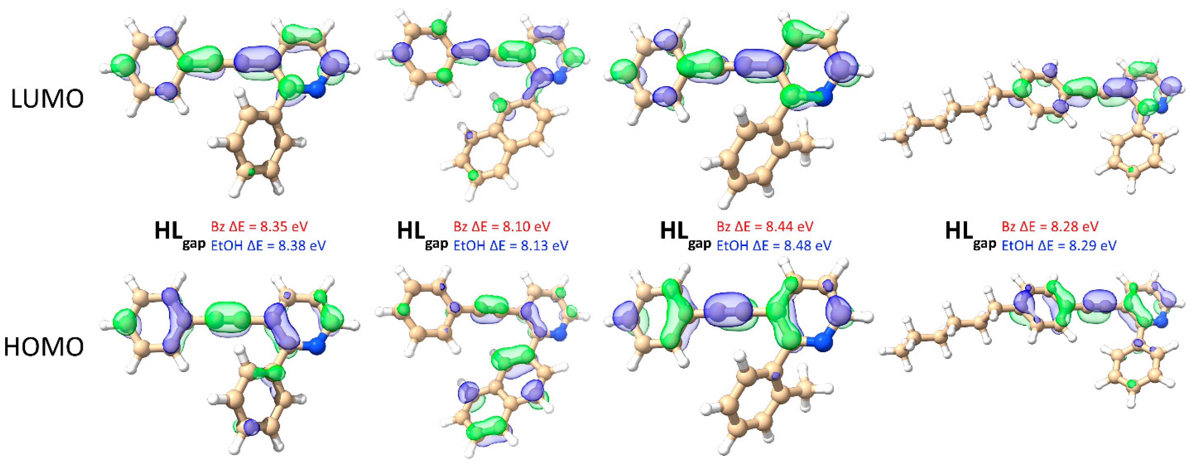
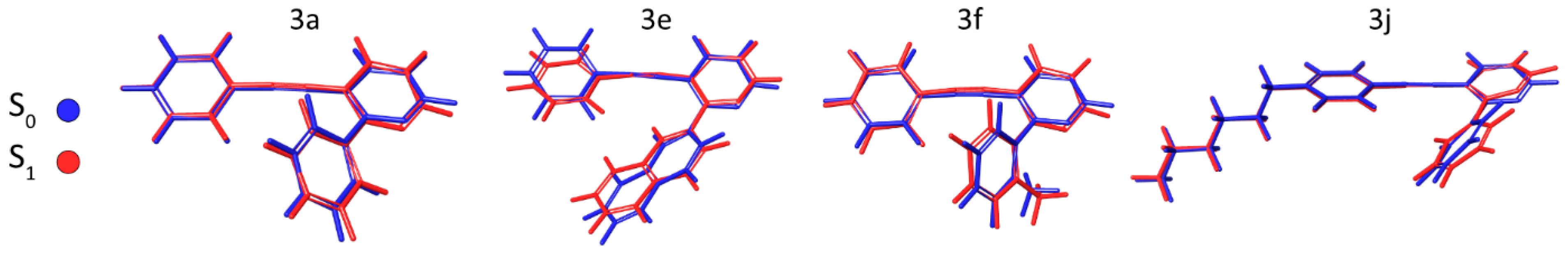
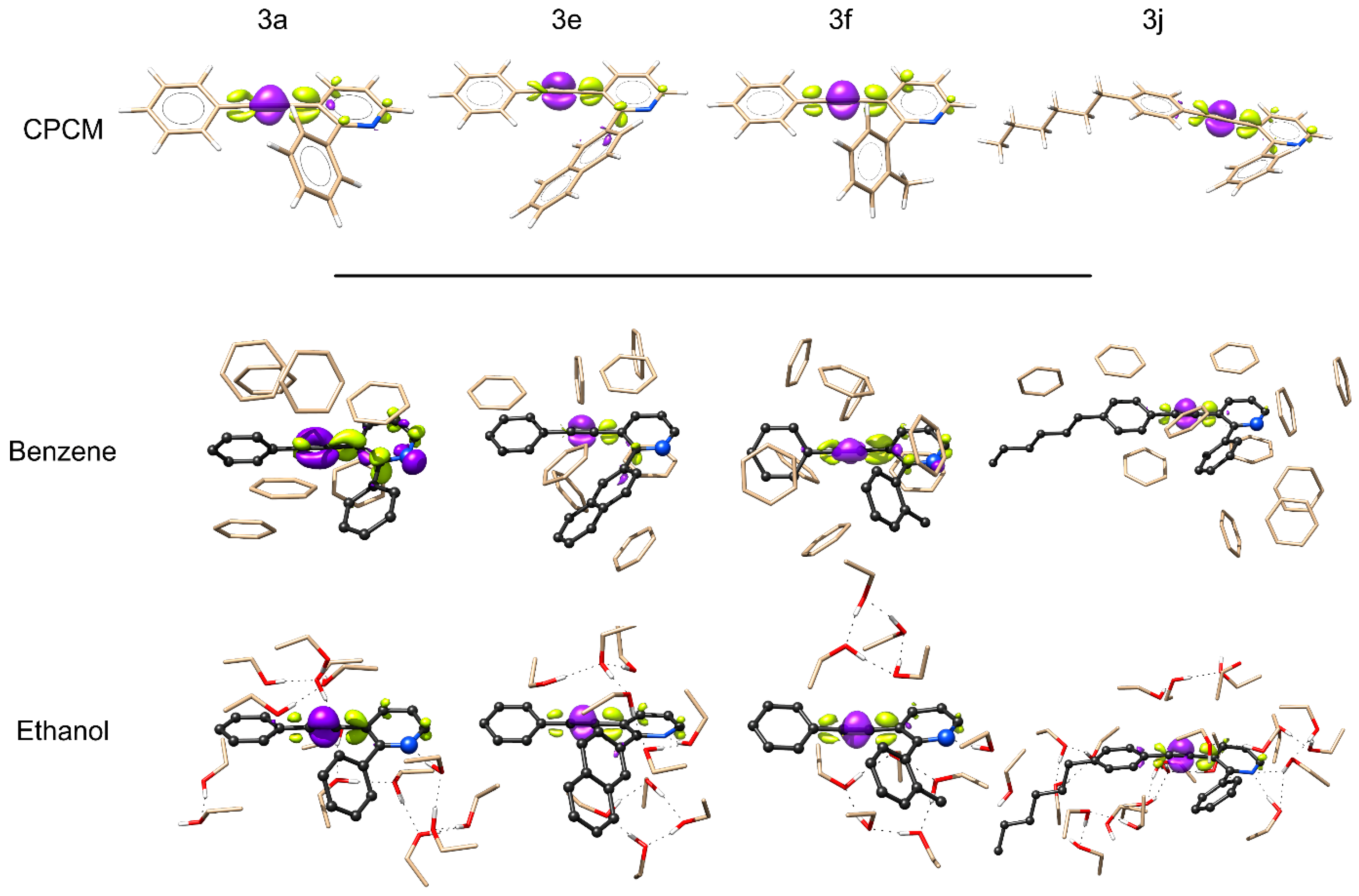
3.3. Theoretical Calculations
4. Conclusions
Supplementary Materials
Author Contributions
Funding
Acknowledgments
Conflicts of Interest
References
- Kalligeros, S.; Zannikos, F.; Stournas, S.; Lois, E. Fuel adulteration issues in Greece. Energy 2003, 28, 15–26. [Google Scholar] [CrossRef]
- Obeidat, S.M.; Al-Ktash, M.M.; Al-Momani, I.F. Study of Fuel Assessment and Adulteration Using EEMF and Multiway PCA. Energy Fuels 2014, 28, 4889–4894. [Google Scholar] [CrossRef]
- Mendes, G.; Barbeira, P.J.S. Detection and quantification of adulterants in gasoline using distillation curves and multivariate methods. Fuel 2013, 112, 163–171. [Google Scholar] [CrossRef] [Green Version]
- Barbeira, P.J.S.; Pereira, R.C.C.; Corgozinho, C.N.C. Identification of Gasoline Origin by Physical and Chemical Properties and Multivariate Analysis. Energy Fuels 2007, 21, 2212–2215. [Google Scholar] [CrossRef]
- Zanelli, A.; Bassini, S.; Giorgetti, M.; Li, Y.; Yang, M.J. Chemiresistors for ethanol detection in hydrocarbons. Sens. Actuators B Chem. 2010, 148, 147–152. [Google Scholar] [CrossRef]
- Wiziack, N.K.L.; Catini, A.; Santonico, M.; D’Amico, A.; Paolesse, R.; Paterno, L.G.; Fonseca, F.J.; Di Natale, C. A sensor array based on mass and capacitance transducers for the detection of adulterated gasolines. Sens. Actuators B Chem. 2009, 140, 508–513. [Google Scholar] [CrossRef]
- Benvenho, A.R.V.; Li, R.W.C.; Gruber, J. Polymeric electronic gas sensor for determining alcohol content in automotive fuels. Sens. Actuators B Chem. 2009, 136, 173–176. [Google Scholar] [CrossRef]
- Eaidkong, T.; Mungkarndee, R.; Phollookin, C.; Tumcharern, G.; Sukwattanasinitt, M.; Wacharasindhu, S. Polydiacetylene paper-based colorimetric sensor array for vapor phase detection and identification of volatile organic compounds. J. Mater. Chem. 2012, 22, 5970–5977. [Google Scholar] [CrossRef]
- Suklabaidya, S.; Chakraborty, S.; Sarkar, S.; Paul, R.; Banik, H.; Chakraborty, A.; Bhattacharjee, D.; Majumdar, S.; Hussain, S.A. Polydiacetylene-N-1-hexadecyl Imidazole Mixed Film and its Application Toward the Sensing of Volatile Organic Compounds, Gasoline, and Pollution Level in Car Exhaust. J. Phys. Chem. C 2021, 125, 15976–15986. [Google Scholar] [CrossRef]
- Lee, J.; Balakrishnan, S.; Cho, J.; Jeon, S.-H.; Kim, J.-M. Detection of adulterated gasoline using colorimetric organic microfibers. J. Mater. Chem. 2011, 21, 2648–2655. [Google Scholar] [CrossRef]
- Aristilde, S.; Cordeiro, C.M.B.; Osório, J.H. Gasoline Quality Sensor Based on Tilted Fiber Bragg Gratings. Photonics 2019, 6, 51. [Google Scholar] [CrossRef] [Green Version]
- Nishikawa, M.; Murata, T.; Ishihara, S.; Shiba, K.; Shrestha, L.K.; Yoshikawa, G.; Minami, K.; Ariga, K. Discrimination of Methanol from Ethanol in Gasoline Using a Membrane-type Surface Stress Sensor Coated with Copper(I) Complex. Bull. Chem. Soc. Jpn. 2021, 94, 648–654. [Google Scholar] [CrossRef]
- Regmi, B.P.; Adhikari, P.L.; Dangi, B.B. Ionic Liquid-Based Quartz Crystal Microbalance Sensors for Organic Vapors: A Tutorial Review. Chemosensors 2021, 9, 194. [Google Scholar] [CrossRef]
- Speller, N.C.; Siraj, N.; Vaughan, S.; Speller, L.N.; Warner, I.M. QCM virtual multisensor array for fuel discrimination and detection of gasoline adulteration. Fuel 2017, 199, 38–46. [Google Scholar] [CrossRef]
- Koshets, I.A.; Kazantseva, Z.I.; Shirshov, Y.M.; Cherenok, S.A.; Kalchenko, V.I. Calixarene films as sensitive coatings for QCM-based gas sensors. Sens. Actuators B Chem. 2005, 106, 177–181. [Google Scholar] [CrossRef]
- Nowak, A.V. Method for Determining Adulteration of Gasolines. U.S. Patent 5358873, 27 July 1992. [Google Scholar]
- Albert, B.; Kipper, J.; Vamvakaris, C.; Beck, K.H.; Wagenblast, G. Use of Compounds Which Absorb and/or Fluoresce in the IR Region as Markers for Liquids. U.S. Patent 5998211A, 23 May 2017. [Google Scholar]
- Rodembusch, F.S.; Duarte, R.C. Sensor Óptico Para a Detecção de Adulteração de Gasolina, Processo de Produção de Soluções Contendo um Sensor Óptico, Método de Detecção de Adulteração de Gasolina Automotiva Comum e Uso de um Corante Orgânico Derivado de Heptameteno Cianinas. Patent BR1020170107396, 31 May 2004. [Google Scholar]
- Krutak, J.J.; Cushman, M.R.; Weaver, M.A. Method for Tagging Petroleum Products. Patent WO1996010620A1, 30 September 1994. [Google Scholar]
- Baxter, D.R.; Cranmer, P.J.; Ho, K.S. Método Para Marcação de um Hidrocarboneto Líquido de Petróleo. Patent BR200305751, 31 May 2004. [Google Scholar]
- Gotor, R.; Tiebe, C.; Schlischka, J.; Bell, J.; Rurack, K. Detection of Adulterated Diesel Using Fluorescent Test Strips and Smartphone Readout. Energy Fuels 2017, 31, 11594–11600. [Google Scholar] [CrossRef]
- Isoppo, V.G.; Gil, E.S.; Gonçalves, P.F.B.; Rodembusch, F.S.; Moro, A.V. Highly fluorescent lipophilic 2,1,3-benzothiadiazole fluorophores as optical sensors for tagging material and gasoline adulteration with ethanol. Sens. Actuators B Chem. 2020, 309, 127701. [Google Scholar] [CrossRef]
- Gotor, R.; Bell, J.; Rurack, K. Tailored fluorescent solvatochromic test strips for quantitative on-site detection of gasoline fuel adulteration. J. Mater. Chem. C 2019, 7, 2250–2256. [Google Scholar] [CrossRef] [Green Version]
- Mineo, P.G.; Vento, F.; Abbadessa, A.; Scamporrino, E.; Nicosia, A. An optical sensor of acidity in fuels based on a porphyrin derivative. Dyes Pigment. 2019, 161, 147–154. [Google Scholar] [CrossRef]
- Huang, Y.; He, J.; Qin, T.; Xiang, X.; Liu, B.; Wang, L. Fluorescence Determination of Ethanol-Gasoline Blends without the Aid of Excitation-Emission Matrix Fluorescence. Chem. Lett. 2019, 48, 1383–1386. [Google Scholar] [CrossRef]
- Düwel, I.; Schorr, J.; Peuser, P.; Zeller, P.; Wolfrum, J.; Schulz, C. Spray Diagnostics Using an All-Solid-State Nd:YAlO3 Laser and Fluorescence Tracers in Commercial Gasoline and Diesel Fuels. Appl. Phys. B 2004, 79, 249–254. [Google Scholar] [CrossRef]
- Galgano, P.D.; Loffredo, C.; Sato, B.M.; Reichardt, C.; El Seoud, O.A. Introducing education for sustainable development in the undergraduate laboratory: Quantitative analysis of bioethanol fuel and its blends with gasoline by using solvatochromic dyes. Chem. Educ. Res. Pract. 2012, 13, 147–153. [Google Scholar] [CrossRef]
- Kumar, K.; Mishra, A.K. Quantification of ethanol in petrol–ethanol blends: Use of Reichardt’s ET(30) dye in introducing a petrol batch independent calibration procedure. Talanta 2012, 100, 414–418. [Google Scholar] [CrossRef]
- Budag, R.; Giusti, L.A.; Machado, V.G.; Machado, C. Quality analysis of automotive fuel using solvatochromic probes. Fuel 2006, 85, 1494–1497. [Google Scholar] [CrossRef]
- Wang, X.; Sun, G.; Routh, P.; Kim, D.-H.; Huang, W.; Chen, P. Heteroatom-doped graphene materials: Syntheses, properties and applications. Chem. Soc. Rev. 2014, 43, 7067–7098. [Google Scholar] [CrossRef] [PubMed] [Green Version]
- Maiti, U.N.; Lee, W.J.; Lee, J.M.; Oh, Y.; Kim, J.Y.; Kim, J.E.; Shim, J.; Han, T.H.; Kim, S.O. 25th Anniversary Article: Chemically Modified/Doped Carbon Nanotubes & Graphene for Optimized Nanostructures & Nanodevices. Adv. Mater. 2014, 26, 40–67. [Google Scholar] [CrossRef]
- Duan, J.; Chen, S.; Jaroniec, M.; Qiao, S.Z. Heteroatom-Doped Graphene-Based Materials for Energy-Relevant Electrocatalytic Processes. ACS Catal. 2015, 5, 5207–5234. [Google Scholar] [CrossRef]
- Qian, G.; Wang, Z.Y. Near-Infrared Organic Compounds and Emerging Applications. Chem. Asian J. 2010, 5, 1006–1029. [Google Scholar] [CrossRef]
- Pawlicki, M.; Collins, H.A.; Denning, R.G.; Anderson, H.L. Two-Photon Absorption and the Design of Two-Photon Dyes. Angew. Chem. Int. Ed. 2009, 48, 3244–3266. [Google Scholar] [CrossRef]
- Li, Y.; Xiong, J.; Li, S.; Wen, X.; Yu, T.; Lu, Y.; Xiong, X.; Liu, Y.; Xiong, X. Fluorescent difference between two rhodamine-PAHs polystyrene solid-phase sensors for Hg(II) detection based on crystal structure and density functional theory calculation. Spectrochim. Spectrochim. Acta Part A Mol. Biomol. Spectrosc. 2020, 234, 118277. [Google Scholar] [CrossRef]
- Roncali, J. Synthetic Principles for Bandgap Control in Linear π-Conjugated Systems. Chem. Rev. 1997, 97, 173–206. [Google Scholar] [CrossRef] [PubMed]
- Bronner, C.; Stremlau, S.; Gille, M.; Brauße, F.; Haase, A.; Hecht, S.; Tegeder, P. Aligning the Band Gap of Graphene Nanoribbons by Monomer Doping. Angew. Chem. Int. Ed. 2013, 52, 4422–4425. [Google Scholar] [CrossRef] [PubMed]
- Miao, Q. Ten Years of N-Heteropentacenes as Semiconductors for Organic Thin-Film Transistors. Adv. Mater. 2014, 26, 5541–5549. [Google Scholar] [CrossRef] [PubMed]
- Verbitskiy, E.V.; Steparuk, A.S.; Zhilina, E.F.; Emets, V.V.; Grinberg, V.A.; Krivogina, E.V.; Kozyukhin, S.A.; Belova, E.V.; Lazarenko, P.I.; Rusinov, G.L.; et al. Pyrimidine-Based Push–Pull Systems with a New Anchoring Amide Group for Dye-Sensitized Solar Cells. Electron. Mater. 2021, 2, 142–153. [Google Scholar] [CrossRef]
- Ding, X.; Wang, H.; Chen, C.; Li, H.; Tian, Y.; Li, Q.; Wu, C.; Ding, L.; Yang, X.; Cheng, M. Passivation functionalized phenothiazine-based hole transport material for highly efficient perovskite solar cell with efficiency exceeding 22%. Chem. Eng. J. 2021, 410, 128328. [Google Scholar] [CrossRef]
- Verbitskiy, E.V.; Rusinov, G.L.; Chupakhin, O.N.; Charushin, V.N. Azines as unconventional anchoring groups for dye-sensitized solar cells: The first decade of research advances and a future outlook. Dyes Pigment. 2021, 194, 109650. [Google Scholar] [CrossRef]
- Li, W.; Shen, C.; Wu, Z.; Wang, Y.; Ma, D.; Wu, Y. Pyridine functionalized phenothiazine derivatives as low-cost and stable hole-transporting material for perovskite solar cells. Mater. Today Energy 2022, 23, 100903. [Google Scholar] [CrossRef]
- Verbitskiy, E.V.; Rusinov, G.L.; Chupakhin, O.N.; Charushin, V.N. Design of fluorescent sensors based on azaheterocyclic push-pull systems towards nitroaromatic explosives and related compounds: A review. Dyes Pigment. 2020, 180, 108414. [Google Scholar] [CrossRef]
- Dhiman, S.; Singla, N.; Ahmad, M.; Singh, P.; Kumar, S. Protonation- and electrostatic-interaction-based fluorescence probes for the selective detection of picric acid (2,4,6-trinitrophenol)–an explosive material. Mater. Adv. 2021, 2, 6466–6498. [Google Scholar] [CrossRef]
- Mahmood, A.; Irfan, A.; Wang, J.L. Developing Efficient Small Molecule Acceptors with sp2-Hybridized Nitrogen at Different Positions by Density Functional Theory Calculations, Molecular Dynamics Simulations and Machine Learning. Chem. Eur. J. 2022, 28, e202103712. [Google Scholar] [CrossRef]
- Motoyama, M.; Doan, T.-H.; Hibner-Kulicka, B.; Otake, R.; Lukarska, M.; Lohier, J.-F.; Ozawa, K.; Nanbu, S.; Alayrac, C.; Suzuki, Y.; et al. Synthesis and Structure-Photophysics Evaluation of 2-N-amino-quinazolines: Small Molecule Fluorophores for Solution and Solid State. Chem. Asian J. 2021, 16, 2087–2099. [Google Scholar] [CrossRef]
- De Salles, H.D.; Coelho, F.L.; Paixão, D.B.; Barboza, C.A.; Rampon, D.D.S.; Rodembusch, F.S.; Schneider, P.H. Evidence of a Photoinduced Electron-Transfer Mechanism in the Fluorescence Self-quenching of 2,5-Substituted Selenophenes Prepared through In Situ Reduction of Elemental Selenium in Superbasic Media. J. Org. Chem. 2021, 86, 10140–10153. [Google Scholar] [CrossRef] [PubMed]
- Radatz, C.S.; Coelho, F.L.; Gil, E.S.; Santos, F.D.S.; Schneider, J.M.F.M.; Gonçalves, P.F.B.; Rodembusch, F.; Schneider, P.H. Ground and excited-state properties of 1,3-benzoselenazole derivatives: A combined theoretical and experimental photophysical investigation. J. Mol. Struct. 2020, 1207, 127817. [Google Scholar] [CrossRef]
- Rampon, D.S.; Rodembusch, F.S.; Gonçalves, P.F.B.; Lourega, R.V.; Merlo, A.A.; Schneider, P.H. An evaluation of the chalcogen atom effect on the mesomorphic and electronic properties in a new homologous series of chalcogeno esters. J. Braz. Chem. Soc. 2010, 21, 2100–2107. [Google Scholar] [CrossRef] [Green Version]
- Peglow, T.J.; Martins, C.C.; da Motta, K.P.; Luchese, C.; Wilhelm, E.A.; Stieler, R.; Schneider, P.H. Synthesis and biological evaluation of 5-chalcogenyl-benzo[h]quinolines via photocyclization of arylethynylpyridine derivatives. New J. Chem. 2022, 46, 23030–23038. [Google Scholar] [CrossRef]
- Armarego, W.L.F. Purification of Laboratory Chemicals, 8th ed.; Butterworth-Heinemann: Oxford, UK, 2017. [Google Scholar]
- Peglow, T.J.; Bartz, R.H.; Martins, C.C.; Belladona, A.L.; Luchese, C.; Wilhelm, E.A.; Schumacher, R.F.; Perin, G. Synthesis of 2-Organylchalcogenopheno [2,3-b]pyridines from Elemental Chalcogen and NaBH4/PEG-400 as a Reducing System: Antioxidant and Antinociceptive Properties. ChemMedChem 2020, 15, 1741–1751. [Google Scholar] [CrossRef]
- Peglow, T.J.; Bartz, R.H.; Barcellos, T.; Schumacher, R.F.; Cargnelutti, R.; Perin, G. Synthesis of 2-Aryl-(3-organochalcogenyl)thieno [2,3-b] pyridines Promoted by Oxone®. Asian J. Org. Chem. 2021, 10, 1198–1206. [Google Scholar] [CrossRef]
- Queiroz, M.-J.R.P.; Begouin, A.; Peixoto, D. Regiocontrolled SNAr Reaction on 2,3-Dihalopyridines with NaSMe To Obtain Bromo(methylthio)pyridines as Key Precursors of 3-Halo-2-(hetero)arylthieno[2,3-b]pyridines and Thieno[3,2-b]pyridines. Synthesis 2013, 45, 1489–1496. [Google Scholar] [CrossRef]
- Peixoto, D.; Begouin, A.; Queiroz, M.-J.R. Synthesis of 2- arylthieno[2,3-b] [2,3-b] or [3,2-b]pyridines from 2,3-dihalopyridines, (hetero)arylalkynes, and Na2S. Further functionalizations. Tetrahedron 2012, 68, 7082–7094. [Google Scholar] [CrossRef] [Green Version]
- Molenda, R.; Boldt, S.; Villinger, A.; Ehlers, P.; Langer, P. Synthesis of 2-Azapyrenes and Their Photophysical and Electrochemical Properties. J. Org. Chem. 2020, 85, 12823–12842. [Google Scholar] [CrossRef]
- Neese, F. The ORCA Program System. WIREs Comput. Mol. Sci. 2012, 2, 73–78. [Google Scholar] [CrossRef]
- Neese, F. Software Update: The ORCA Program System, version 4.0. WIREs Comput. Mol. Sci. 2018, 8, e1327. [Google Scholar] [CrossRef]
- Neese, F.; Wennmohs, F.; Becker, U.; Riplinger, C. The ORCA quantum chemistry program package. J. Chem. Phys. 2020, 152, 224108. [Google Scholar] [CrossRef] [PubMed]
- Pracht, P.; Bohle, F.; Grimme, S. Automated exploration of the low-energy chemical space with fast quantum chemical methods. Phys. Chem. Chem. Phys. 2020, 22, 7169–7192. [Google Scholar] [CrossRef]
- Ehlert, S.; Stahn, M.; Spicher, S.; Grimme, S. Robust and Efficient Implicit Solvation Model for Fast Semiempirical Methods. J. Chem. Theory Comput. 2021, 17, 4250–4261. [Google Scholar] [CrossRef]
- Lin, Y.-S.; Li, G.-D.; Mao, S.-P.; Chai, J.-D. Long-Range Corrected Hybrid Density Functionals with Improved Dispersion Corrections. J. Chem. Theory Comput. 2013, 9, 263–272. [Google Scholar] [CrossRef]
- Weigend, F.; Ahlrichs, R. Balanced basis sets of split valence, triple zeta valence and quadruple zeta valence quality for H to Rn: Design and assessment of accuracy. Phys. Chem. Chem. Phys. 2005, 7, 3297–3305. [Google Scholar] [CrossRef]
- Takano, Y.; Houk, K.N. Benchmarking the Conductor-like Polarizable Continuum Model (CPCM) for Aqueous Solvation Free Energies of Neutral and Ionic Organic Molecules. J. Chem. Theory Comput. 2005, 1, 70–77. [Google Scholar] [CrossRef]
- Hirata, S.; Head-Gordon, M. Time-dependent density functional theory within the Tamm–Dancoff approximation. Chem. Phys. Lett. 1999, 314, 291–299. [Google Scholar] [CrossRef]
- Shibata, T.; Takayasu, S.; Yuzawa, S.; Otani, T. Rh(III)-Catalyzed C-H Bond Activation Along with “Rollover” for the Synthesis of 4-Azafluorenes. Org. Lett. 2012, 14, 5106–5109. [Google Scholar] [CrossRef]
- Shestakov, A.N.; Pankova, A.S.; Kuznetsov, M.A. Cycloisomerization–a straightforward way to benzo[h]quinolines and benzo[c]acridines. Chem. Heterocycl. Compd. 2017, 53, 1103–1113. [Google Scholar] [CrossRef]
- Smith, M.T. Advances in Understanding Benzene Health Effects and Susceptibility. Annu. Rev. Public Health 2010, 31, 133–148. [Google Scholar] [CrossRef] [Green Version]
- Lachenmeier, D.W.; Reusch, H.; Sproll, C.; Schoeberl, K.; Kuballa, T. Occurrence of benzene as a heat-induced contaminant of carrot juice for babies in a general survey of beverages. Food Addit. Contam. Part A 2008, 25, 1216–1224. [Google Scholar] [CrossRef]
- Dos Santos, V.P.S.; Salgado, A.M.; Torres, A.G.; Pereira, K.S. Benzene as a Chemical Hazard in Processed Foods. Int. J. Food Sci. 2015, 2015, 545640. [Google Scholar] [CrossRef] [PubMed]
- Sadighara, P.; Pirhadi, M.; Sadighara, M.; Shavaly-Gilani, P.; Zirak, M.R.; Zeinali, T. Benzene food exposure and their prevent methods: A review. Nutr. Food Sci. 2022, 52, 971–979. [Google Scholar] [CrossRef]
- Gehlen, M.H. The centenary of the Stern-Volmer equation of fluorescence quenching: From the single line plot to the SV quenching map. J. Photochem. Photobiol. C Photochem. Rev. 2020, 42, 100338. [Google Scholar] [CrossRef]
- Luria, M.; Ofran, M.; Stein, G. Natural and experimental fluorescence lifetimes of benzene in various solvents. J. Phys. Chem. 1974, 78, 1904–1909. [Google Scholar] [CrossRef]
- Montalti, M.; Credi, A.; Prodi, L.; Gandolfi, M.T. Handbook of Photochemistry, 3rd ed.; CRC Press: Boca Raton, FL, USA, 2006. [Google Scholar]
- How to Determine the LOD Using the Calibration Curve? Available online: https://mpl.loesungsfabrik.de/en/english-blog/method-validation/calibration-line-procedure (accessed on 9 February 2023).
- Mistura Carburante (Etanol Anidro-Gasolina) Cronologia. Available online: http://www.agricultura.gov.br/assuntos/sustentabilidade/agroenergia/arquivos/cronologia-da-mistura-carburante-etanol-anidro-gasolina-no-brasil.pdf (accessed on 11 January 2023).
- Ho, J.; Ertem, M.Z. Calculating Free Energy Changes in Continuum Solvation Models. J. Phys. Chem. B 2016, 120, 1319–1329. [Google Scholar] [CrossRef]
- De Souza, B.; Neese, F.; Izsák, R. On the theoretical prediction of fluorescence rates from first principles using the path integral approach. J. Chem. Phys. 2018, 148, 034104. [Google Scholar] [CrossRef] [PubMed]


| Fluorophores | 3a | 3b | 3c | 3d | 3e | 3f | 3g | 3h | 3i | 3j | 3k |
|---|---|---|---|---|---|---|---|---|---|---|---|
| Benzene | |||||||||||
| λabs | 298 | 300 | 300 | 296 | 308 | 303 | 306 | 301 | 303 | 278 | 299 |
| ε | 15,300 | 10,691 | 15,155 | 13,381 | 12,963 | 15,972 | 12,214 | 16,554 | 16,634 | 9706 | 15,051 |
| λem | 355 | 360 | 368 | 375 | 378 | 346 | 368 | 363 | 364 | 317 | 365 |
| ΔλST | 57/5388 | 60/5556 | 68/6159 | 79/7117 | 70/5942 | 43/3592 | 62/5506 | 62/5674 | 61/5531 | 39/4425 | 66/6048 |
| Ethanol | |||||||||||
| λabs | 294 | 296 | 295 | 302 | 305 | 305 | 304 | 298 | 299 | 295 | 295 |
| ε | 15,938 | 9829 | 15,684 | 12,860 | 10,484 | 14,123 | 14,278 | 15,174 | 16,634 | 10,802 | 15,532 |
| λem | 361 | 357 | 373 | 376 | 377 | 340 | 357 | 369 | 365 | 340 | 367 |
| ΔλST | 67/6313 | 61/5773 | 78/7089 | 74/6517 | 72/5760 | 35/3375 | 53/4884 | 71/6457 | 66/6048 | 45/4487 | 72/6650 |
| Hexane | |||||||||||
| λabs | 296 | 298 | 298 | 302 | 308 | 305 | 304 | 299 | 302 | 266 | 297 |
| ε | 13,706 | 11,898 | 16,917 | 15,814 | 13,153 | 14,459 | 12,730 | 17,244 | 16,802 | 10,802 | 15,532 |
| λem | 337 | 338 | 338 | 358 | 370 | 337 | 339 | 338 | 359 | 310 | 338 |
| ΔλST | 41/4110 | 40/3971 | 40/3971 | 56/6658 | 62/6082 | 32/3113 | 35/3396 | 39/3859 | 57/5257 | 44/5336 | 41/4084 |
| Dichloromethane | |||||||||||
| λabs | 297 | 298 | 298 | 302 | 309 | 297 | 306 | 300 | 302 | 265 | 297 |
| ε | 10,838 | 13,450 | 16,388 | 16,162 | 11,819 | 11,433 | 14,794 | 16,899 | 15,962 | 8610 | 15,692 |
| λem | 360 | 361 | 373 | 378 | 379 | 346 | 368 | 372 | 364 | 344 | 365 |
| ΔλST | 63/5892 | 63/5856 | 75/6747 | 76/6658 | 70/3461 | 49/4768 | 62/5506 | 72/6452 | 62/5640 | 79/8666 | 68/6273 |
| Fluorophores | Range (Benzene %) | KSV (M−1) | kq (M−1·s−1) | LOD 1 (Benzene %) |
|---|---|---|---|---|
| 3c | 0–80 | 0.090 | 9.0 × 10⁶ | 4.6 |
| 3e | 10–45 | 0.021 | 2.1 × 10⁶ | 6.0 |
| 3e | 30–80 | 0.054 | 5.4 × 10⁶ | 12.1 |
| 3i | 0–80 | 0.051 | 5.1 × 10⁶ | 7.4 |
Disclaimer/Publisher’s Note: The statements, opinions and data contained in all publications are solely those of the individual author(s) and contributor(s) and not of MDPI and/or the editor(s). MDPI and/or the editor(s) disclaim responsibility for any injury to people or property resulting from any ideas, methods, instructions or products referred to in the content. |
© 2023 by the authors. Licensee MDPI, Basel, Switzerland. This article is an open access article distributed under the terms and conditions of the Creative Commons Attribution (CC BY) license (https://creativecommons.org/licenses/by/4.0/).
Share and Cite
Peglow, T.J.; Vieira, M.M.; Padilha, N.B.; Dalberto, B.T.; Silva Júnior, H.d.C.; Rodembusch, F.S.; Schneider, P.H. Pyridine-Based Small-Molecule Fluorescent Probes as Optical Sensors for Benzene and Gasoline Adulteration. Photochem 2023, 3, 109-126. https://doi.org/10.3390/photochem3010008
Peglow TJ, Vieira MM, Padilha NB, Dalberto BT, Silva Júnior HdC, Rodembusch FS, Schneider PH. Pyridine-Based Small-Molecule Fluorescent Probes as Optical Sensors for Benzene and Gasoline Adulteration. Photochem. 2023; 3(1):109-126. https://doi.org/10.3390/photochem3010008
Chicago/Turabian StylePeglow, Thiago Jacobsen, Marcelo Marques Vieira, Nathalia Batista Padilha, Bianca T. Dalberto, Henrique de Castro Silva Júnior, Fabiano Severo Rodembusch, and Paulo Henrique Schneider. 2023. "Pyridine-Based Small-Molecule Fluorescent Probes as Optical Sensors for Benzene and Gasoline Adulteration" Photochem 3, no. 1: 109-126. https://doi.org/10.3390/photochem3010008