Measurement Precision and Thermal and Absorption Properties of Nanostructures in Aqueous Solutions by Transient and Steady-State Thermal-Lens Spectrometry

Abstract

A simultaneous steady-state and transient photothermal-lens modality was used for both the thermal and optical parameters of aqueous dispersed systems (carbon and silica nanoparticles, metal iodides, surfactants, heme proteins, albumin, and their complexes). Heat-transfer parameters (thermal diffusivity and thermal effusivity), the temperature gradient of the refractive index, light absorption, and concentration parameters were assessed. To simultaneously measure thermal and optical parameters, the time scale of thermal lensing (characteristic time, $t_c$) should correspond to an excitation beam size of 60–300 µm, and the relative time intervals $\left(0.5÷5\right)t_c$ and (5$÷20)t_c$ should be selected for transient and steady-state measurements, respectively. Dual-beam thermal-lens spectrometers in a mode-mismatched optical schematic at various excitation wavelengths were built. The spectrometers implement back-synchronized detection, providing different measurement conditions for the heating and cooling parts of the thermal-lens cycle. By varying the measurement parameters depending on the dispersed system, the conditions providing the suitable precision (replicability, repeatability, and reproducibility) of thermal-lens measurements were found; setups with a broad excitation beam (waist size, 150 and 300 μm) provide longer times to attain a thermal equilibrium and, thus, the better precision of measurements of thermal diffusivity.

1. Introduction

Thermal-lens (photothermal-lens) spectrometry (TLS), as a high-sensitivity nondestructive technique of molecular absorption spectroscopy, has evolved into a versatile method [1,2,3,4,5,6]. TLS, as the most widespread photothermal technique, has two advantages over conventional (transmission) methods of molecular absorption spectroscopy (UV/vis photometry and IR spectroscopy) [1,7,8,9,10,11]. The first is considerably higher sensitivity because TLS is based on direct measurements of the nonradiative energy transfer from excited chromophore molecules [2,3,4,12,13]. Thermal relaxation in the sample results in a nonuniform refractive-index spatial profile (a thermal-lens effect). Its optical strength is proportional to the sample absorbance and, thus, to the absorber concentration and its absorptivity. As a result, TLS provides detection limits of 10⁻⁹–10⁻⁶ abs. units or ca. 10⁻¹¹ mol L⁻¹ [2,10,14,15,16,17,18], i.e., a sensitivity that is comparable to that of laser-induced fluorimetry but for non-fluorescing chromophores and with the low impact of light scattering [19,20]. The second advantage of TLS is the possibility of measuring chromophore absorption in complex (even living) systems and in vivo studies [11,21,22,23,24,25], also with the low impact of scattering backgrounds [26,27]. The high sensitivity of measurements is achieved not only through instrumentation but also because of more advantageous reaction conditions at trace levels and a reaction medium with advantageous thermophysical properties [2,28], which lowers the limits of detection and quantification for various substances [2,16,29,30,31,32,33,34,35,36,37,38]. Since the 1980s, TLS has been used in analytical and physical–chemistry applications, including highly sensitive quantification, adaptable detection schemes in various separation techniques, including microfluidics, and multiple biomedical tasks [4,8,39,40,41,42]. In addition, much attention has been paid to applications in microfluidic systems (chemical microchips or µTAS) [43]. TLS is used for assessing the spectral parameters of dispersed solutions [20,44,45] including proteins and blood components [46,47].

However, TLS also serves as a method of thermal spectroscopy, and the signal in TLS depends not only on absorption but also on the photothermal properties of the medium: thermal properties, thermal conductivity, thermal diffusivity, thermal effusivity, and the temperature gradient of the refractive index (thermo-optical constant), as well as the density and absorption-to-heat conversion [4,6,15,33,48,49,50,51,52,53,54,55,56,57,58,59,60,61,62,63,64,65,66]. These response features are implemented as functions of dynamic (transient profile of probe-beam defocusing, transient TLS [59,67,68,69,70,71,72,73,74,75]) and static (amplitude fluctuation of the temperature/refractive-index field due to the thermal-lens effect, steady-state TLS [2]). TLS is used for the thermal diffusivity of two-phase systems containing nanoparticles of metals or their oxides [4,29,48,52,53,72,76,77,78,79,80,81,82].

For thermal-lens measurements of dispersed solutions, the spatial distribution of thermal properties in the medium is crucial. Thus, the TLS application for dispersed systems is usually based on high-precision microscopic techniques combined with data visualization and sophisticated data treatment [32,83,84,85,86,87,88,89,90,91,92]. Still, TLS can be implemented with relatively simple dual-beam setups that provide the required sensitivity in rather large-volume bulk samples [2,12,16,93,94]. This approach is considered relatively straightforward for the determination of optical absorption and analyte assessment (similarly to transmission photometry) and is used for the estimation of these properties of solvents. Still, the complex and dynamic nature of photothermal effects provides very informative data, which can be used, even with a non-microscopic schematic, to assess more detailed information: absorption, thermophysical properties, and size parameters [4,50,95,96,97].

A thermal-lens schematic includes a unit to synchronize the start of the blooming of the thermal-lens effect by the excitation beam and a pulse from the excitation laser or a modulated (chopped) cw beam. The principles of the most common thermal-lens schematic can be described as a directly synchronized (lock-in) TLS technique, as the primary trigger for a new measurement cycle is a new laser pulse or a modulator opening, and the measurements are made at a constant frequency determined by the pulse repetition rate or a modulator [2,89,94]. This schematic is simple and reliable and provides high sensitivity [86,98]. However, for TLS, single-frequency synchronization may not capture information for complex samples, in which the transient and steady-state responses depend on both optical and thermal heterogeneity [2,99]. Furthermore, for dispersed solutions at a constant frequency, the measurement error may accumulate over time due to incomplete heat dissipation from cycle to cycle, providing a lower temperature response [2,28]. This, in turn, leads to thermally induced processes that result in an uncontrolled contribution to probe-beam blooming.

The back-synchronized measurement excitation/data-treatment technique differs at the start of a new measurement cycle; its start is governed by reaching steady-state thermal-lens conditions [100,101]. In this technique, the advantages are (i) the possibility of simultaneously using transient and repeated steady-state measurements; (ii) a linear dynamic range of more than five orders of magnitude of detectable absorbances, including strongly absorbing and scattering samples; and (iii) the possibility of detection under batch and flow conditions with no change in the optical-scheme design of the instrument [102]. Although the detection sensitivity is somewhat lower compared to more common lock-in schemes [2,89,94], the flexibility of back-synchronized TLS provides a considerably larger information volume for studies of complex formation at trace concentrations or transient heat dynamics around absorbing nanoparticles [84].

In this study, we implemented a simultaneous steady-state and transient photothermal-lens modality for various aqueous dispersions using back-synchronized setups with different time-response scales. The aim was to demonstrate the capability of such a modality for measuring the absorbance and assessing the concentrations of dispersed solutions, along with monitoring the thermal properties (thermal diffusivity and the thermo-optical constant) with the selection of measurement conditions based on precision parameters.

2. Materials and Methods

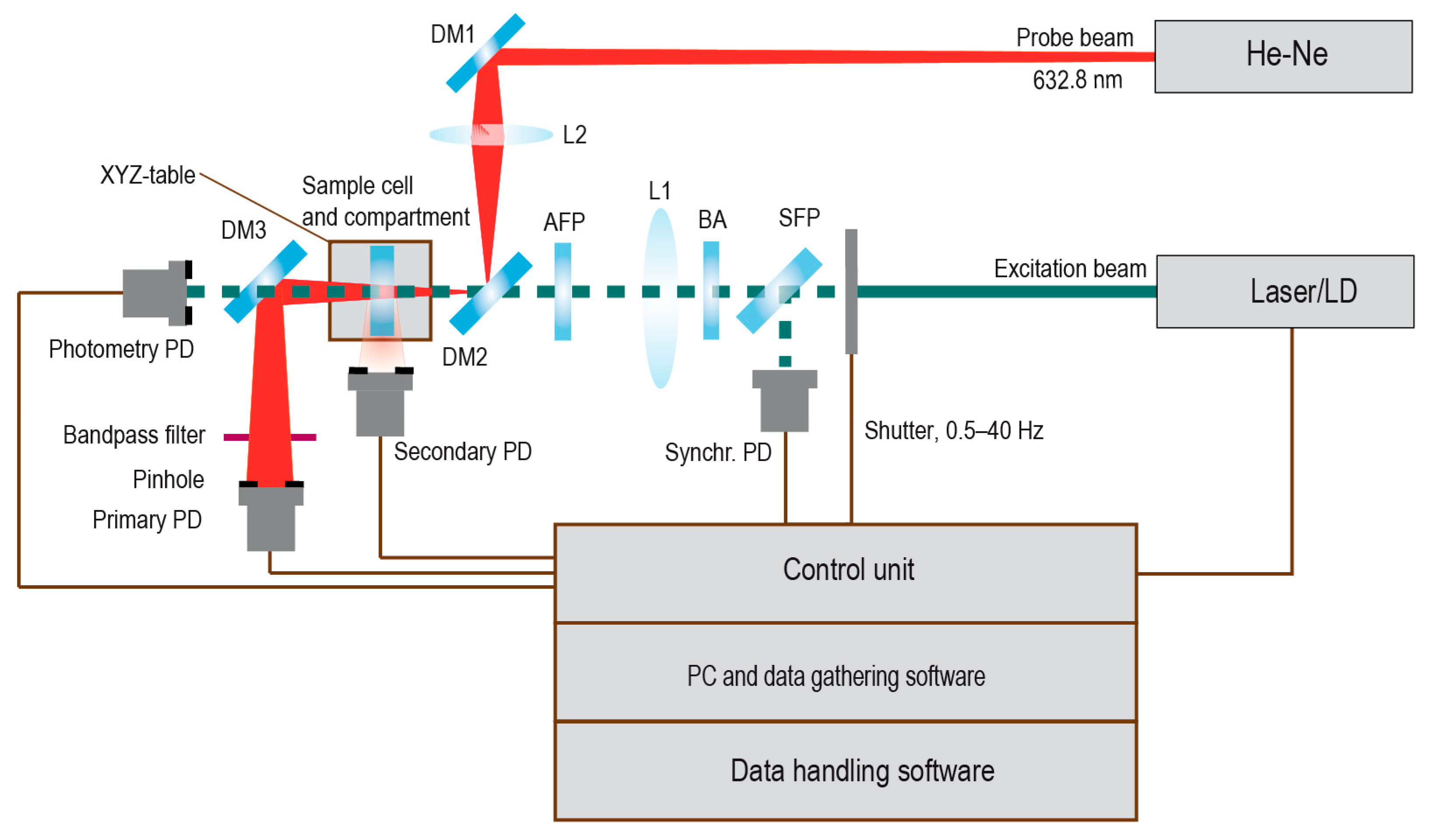
2.1. Thermal-Lens Spectrometer Setups

Thermal-lens spectrometers (the generalized scheme is shown in Figure 1) use a discretely tunable cw Ar⁺ excitation laser (Innova 90-6, Coherent, Palo Alto, CA, USA) with wavelengths (power range in the sample, mW) of 514.5 nm (40–1500), 501.7 nm (5–60), 496.5 nm (4–90), 488.0 nm (5–1000), 476.5 nm (5–82), 472.7 nm (2–20), and 465.8 nm (2–12); an MGL-FN-532 diode-pumped solid-state (DPSS, Changchun New Industries Optoelectronics Tech. Co., Ltd., Changchun, China), TEM₀₀ mode, 532 nm (30–250); and an LSR445NL cw diode-pumped excitation laser, 445 nm (40–450), Q-Baihe (Shenzhen, China). The sample absorption of the excitation radiation induces refractive heterogeneity (the thermal-lens effect), causing the defocusing of a TEM₀₀ He–Ne laser probe beam (HRP020, Thorlabs Inc., Newton, NJ, USA, 632.8 nm). The parameters of the setups are summarized in

Table 1. Parameters of the optical-scheme configuration of dual-beam thermal-lens spectrometers.

Group	Parameter	TLS-60	TLS-150	TLS-300
Excitation laser	Main wavelengths, λe (nm)	488.0, 514.5, and 532.0	488.0, 514.5, and 532.0	445
	Confocal distance zce (mm)	19.5 ± 0.3	130 ± 2	700 ± 10
	Maximum laser power at cell (mW)	1500	250	450
	TEM00 radius at the waist ω0e (µm)	59.8 ± 0.5	150 ± 10	300 ± 10
	Focusing lens focal length fe (mm)	300	330	330
Probe laser	Wavelength λp (nm)	632
	Focusing lens focal length fp (mm)	185	185	100
	Confocal distance zcp (mm)	3.1	3.1	4.46
	Laser power at cell (mW) Pp	3	3	2–4
	Radius at the waist ω0p (µm)	25.0 ± 0.2	25.0 ± 0.2	30.0 ± 0.2
Other parameters	Cell length l, (mm)	10	10	10
	Sample-to-detector distance (cm)	95	47	47
	m, Equation (3)	2.1 ± 0.1	2.9 ± 0.1	2.34 ± 0.08
	V, Equation (3)	3.1 ± 0.1	11.0 ± 0.3	13.0 ± 0.3

. The precision of measurements of optical-scheme parameters is described elsewhere [103].

The excitation beam goes through an electromechanical shutter, is focused with the lens L1 (focal length, 300–330 mm, see Table 1), goes through a dichroic mirror (DM2) of the ZR-100 type (LOMO, St. Petersburg, Russia), and next goes to the sample. A part of excitation beam energy is reflected by the flat plate (SFP) to the synchronizing photodiode (Synchr. PD; L-3DP3C, Panasonic Industrial Devices, Newark, NJ, USA), connected to the control unit. We used the control board of the ADC-DAC unit to synchronize the detection system and the shutter. In setups with argon-ion and Nd-YAG lasers, the power in the cell was adjusted using a neutral-filter beam attenuator (BA). For the fine tuning of the coaxial position, the excitation beam was adjusted with an adjustment flat plate (AFP).

The probe beam is directed to the adjustment dichroic mirror DM1 of the ZR-100 type using a system comprising a dichroic mirror and a focusing lens (L2) (focal length, 100–185 mm). After reaching the sample, the excitation and probe beams are preliminarily separated with a dichroic mirror (DM3) of the ZR-100 type.

The excitation beam is directed to a PD L-3DP3C photodiode (Photometry PD) to account for the excitation beam photometric (transmission) signal (Appendix A). Additionally, this mirror prevents the blooming of the thermal lens in the following bandpass filter. The excitation beam is absorbed by the filter (KS-11 color glass, 2 mm depth). The signal is converted and amplified and enters the ADC-DAC unit. The probe beam passes through a pinhole (diameter, 4 mm) centered at the optical axis and hits the Primary PD L-3DP3C photodiode. The signal is converted and amplified by the control unit and enters Channel 1 of the ADC–DAC unit. Through an amplifier that converts a photocurrent into voltage, the signal from this photodiode enters channel 2 of the ADC and DAC converter, connected to a PC.

Lenses L1 and L2 and the sample compartment can be moved along the directions of the beams (step, 0.2 mm), which provides variation in the spectrometer geometry (degree of mode mismatching, see below). The spectrometer implements a secondary channel (an L-3DP3C photodiode, Secondary PD, Figure 1) for gathering scattering or luminescence signals if present.

A homemade ADC–DAC unit based on a C8051F061 board (two 16-bit ADC and two 12-bit DAC channels, ADC time, 2 µs; readout frequency, 1–5 kHz; C8051F060DK development kit, Silicon Labs, Boston, MA, USA) was used in the external-trigger mode from the PC [100]. The homemade software communicates with the unit through an RS-232 interface. The homemade software is written in C++, Borland C++ ver. 5 (Borland Corp., Austin, TX, USA). After obtaining a full curve of repeated heating–cooling cycles, it is divided into separate cycles; each cycle is divided into heating and cooling half-curves, and each half-cycle curve is divided into transient and steady-state parts. A steady-state signal is calculated automatically during measurements, and the transient curves are treated after the experiment.

2.2. Auxiliary Measurements

An Agilent Cary 4000 spectrophotometer (Agilent, Mulgrave, Australia) was used for UV/Vis spectra recording (l = 1–10 mm, cell volume 0.3 cm³). The pH values were measured by an inoLab pH Level 1 pH-meter (WHW, Weilheim, Germany) with a glass pH-selective electrode (precision ±5%). Solutions were mixed with a Biosan MMS 3000 automatic mixer (Riga, Latvia).

Densities were determined with a VIP-2MP (Termex, Tomsk, Russia) vibrating-tube densimeter. The expression ρ = A + Bτ² was used to obtain the densities of the solutions, where τ is the oscillation period and A and B are coefficients determined from calibration at 298.15 K by known densities and oscillation periods of ambient air, ultrapure water, and standard material, REP-12 (1090.32 kg·m⁻³, produced and certified by D.I. Mendeleev Institute for Metrology, St. Petersburg, Russia). The temperature was maintained by the built-in thermostat; the uncertainty in the temperature was 0.02 °C. The standard deviation for the measurement of the solution density is 0.1 kg·m⁻³. All solutions were homogenized before measurements were taken with a Branson 2510 ultrasonic bath (Danbury, CT, USA).

2.3. Thermal-Lens Data Treatment

The principle of the measurement of steady-state signals and transient thermal-lens curves for the heating and cooling parts of the cycle when the excitation beam is switched on (shutter is opened) and off (shutter is closed), respectively, is depicted in Figure 2. From this point on, the full cycle of the measurement of transient and steady-state thermal-lens signals will be referred to as the excitation on/off cycle.

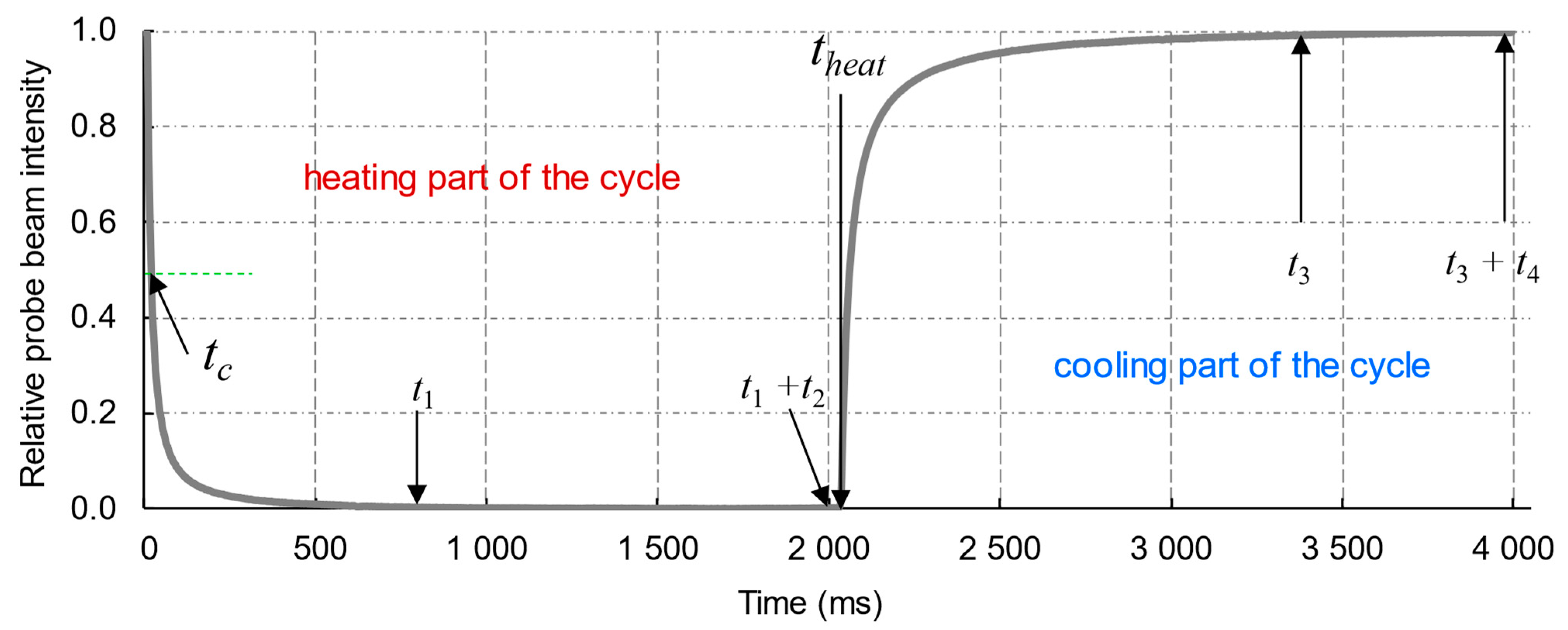
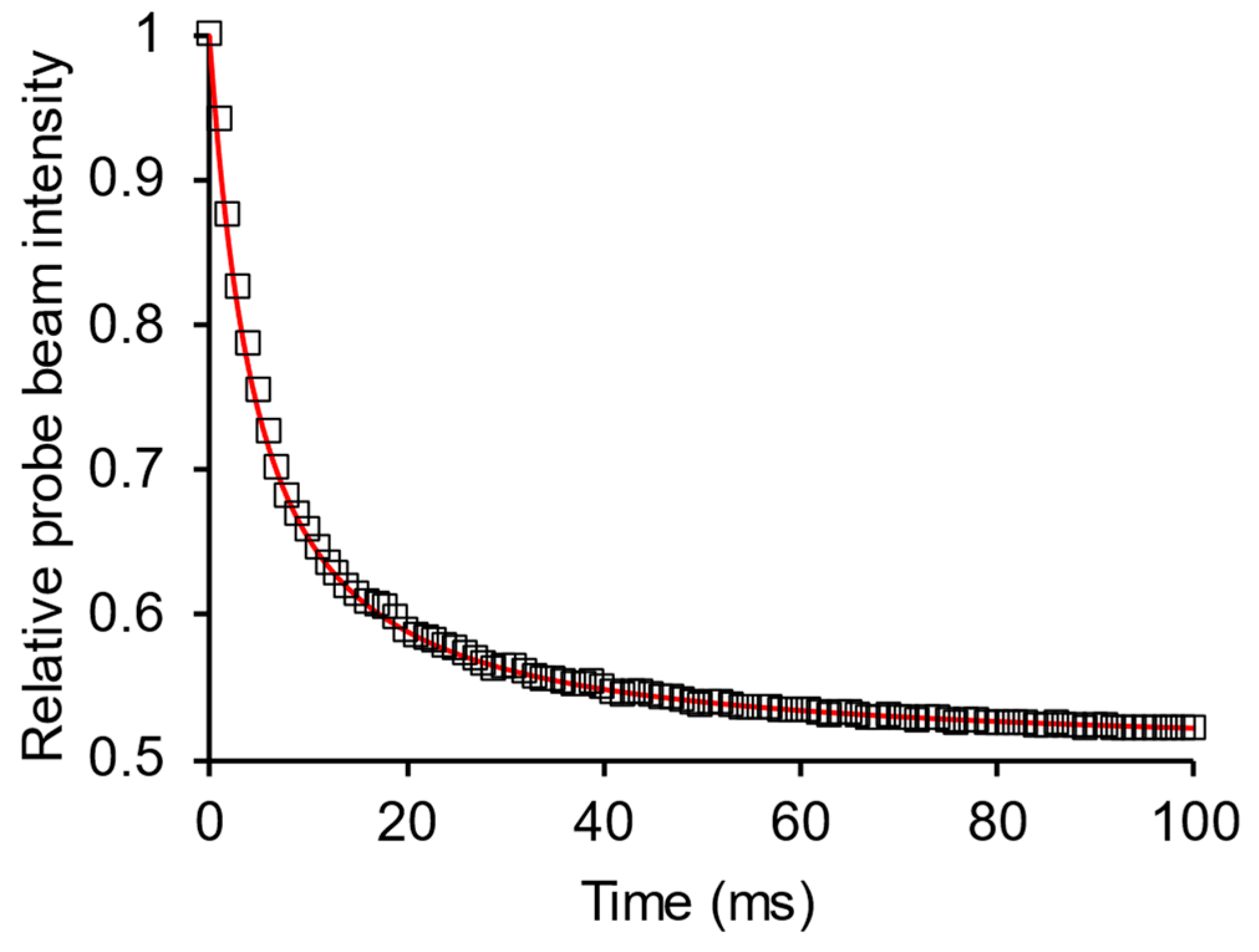
2.3.1. Transient Thermal-Lens Measurements

A transient (time-resolved) thermal-lens signal ϑ(t) for an excitation on/off cycle of a modulated continuous-wave (cw) beam was calculated as the relative change in the probe-beam intensity at a far-field detector plane $I_p\left(t\right)$ at moment t [2]:

$$\vartheta \left(t\right)=\left(I_p\left(0\right)-I_p\left(t\right)\right)/I_p\left(t\right),$$

(1)

where $I_p\left(0\right)$ is the intensity of the probe beam at the photodetector plane in the central part of the beam at time t = 0, and $I_p\left(t\right)$ is the intensity of the probe beam at time t from the excitation on/off cycle start. According to the diffraction model [104,105], the equation for the thermal-lens signal in relation to light absorption and concentration is

$$\vartheta \left(t\right)={\left(1-P_e\cdot ½B\left(t\right)\cdot E_0\cdot \mathsf{\varkappa }l\right)}^{-2}-1={\left(1-P_e\cdot ½B\left(t\right)\cdot E_0\cdot 2.303\epsilon lc\right)}^{-2}-1,$$

(2)

where $P_e$ is the excitation laser power, $\mathsf{\varkappa }=2.303\epsilon c$ is the linear light-absorption coefficient, l is the sample path length, ε is molar absorptivity, and c is molar concentration of the test absorbing substance in the sample. For absorbances up to ca. 0.005, excitation powers up to ca. 200 mW, and, thus, small temperature changes in the thermal-lens effect, Equation (2) can be simplified due to the small contributions of the quadratic terms and can be defined as a linear equation (see Figures S5 and S6, Supplementary Information):

$$\vartheta \left(t\right)=P_e\cdot B\left(t\right)\cdot E_0\cdot \mathsf{\varkappa }l=P_e\cdot B\left(t\right)\cdot E_0\cdot 2.303\epsilon lc,$$

(3)

The factor $E_0$ in Equations (2) and (3) is the power-normalized thermo-optical constant (full thermo-optical constant is $E=P_e{E}_0$), characterizing the strength of the thermal-lens effect per unit excitation laser power, $E_0=\left(-dn/dT\right)/\left({\lambda }_{p}k\right)$. Here, k is the thermal conductivity, ${\lambda }_p$ is the probe-laser wavelength, and the temperature gradient of the refractive index $\left(dn/dT\right)\propto {\mathsf{\alpha }}_T$ (volumetric thermal expansion coefficient).

The parameter $B\left(t\right)$ in Equations (2) and (3) is the time-dependent geometrical constant of the optical schematic [104,105],

$$B\left(t\right)={\tan }^{-1}\left[2mV/\left\{\left[{\left(1+2m\right)}^2+V^2\right]\left(t_c/2t\right)+1+2m+V^2\right\}\right]={\tan }^{-1}\left[a/\left(b{t}_c/2t+c\right)\right].$$

(4)

Here, m is the ratio of the cross-sectional areas of the probe and excitation beams at the sample, and V is the relative distance from the excitation waist to the sample, from the traditional notation of TLS geometry parameters proposed by R. Snook, J. Shen, and M. Baesso [104,105], and a, b, and c are related geometry constants of the spectrometer used in the approximation for equation simplicity’s sake [106].

The parameter $t_c$ in Equation (4) is the characteristic time of the thermal lens [2] and is calculated from the transient curve of thermal-lens measurements (Figure 2).

$$t_c={\omega }_{0e}^2/4D_T,$$

(5)

where ${\omega }_{0e}$ is the excitation beam waist radius, and $D_T$ is thermal diffusivity.

To compare the transient heating and cooling curves under various conditions, we used the relative intensity of the probe beam [107]:

$${\vartheta }_{rel}\left(t\right)=\frac{I_p\left(0\right)-I_p\left(t\right)}{I_p\left(0\right)-I_p\left(\infty \right)},$$

(6)

where $I_p\left(\infty \right)$ is the intensity of the probe beam at thermal equilibrium due to the steady-state thermal-lens effect (t→∞). This form of Equation (1) makes it possible to compare the blooming and dissipation of the curves for various media and with various light absorption characteristics, as all of the curves are normalized to a scale from 0 (fully developed steady-state thermal lens) to 1 (no photothermal effects), thus focusing on differences in the vicinity of the characteristic time $t_c$ of the process.

2.3.2. Steady-State Measurements

The steady-state cw thermal-lens signal is

$$\vartheta =\left(I_p\left(0\right)-I_p\left(\infty \right)\right)/I_p\left(\infty \right),$$

(7)

and, under the same conditions as linear Equation (3), is defined as:

$$\vartheta =P_{e}B{E}_0\mathsf{\varkappa }l=BE\cdot 2.303\epsilon lc=B\mathsf{\theta }.$$

(8)

Here,

$$\mathsf{\theta }\equiv 2.303E_0{P}_e\epsilon lc$$

(9)

is the steady-state thermal-lens signal corrected for the steady-state geometry constant B(t→∞). The calibration plots for TLS were built as $\theta \propto c$ and as a comparison of thermal-lens and transmission measurements (photometry), with

$$\mathsf{\theta }=\kappa A,$$

(10)

where $\kappa$ is a proportionality coefficient, the theoretical value from Equation (9) is $2.303E_0{P}_e$, and A = εlc is absorbance from photometric measurements. The experimental values of the signal θ were corrected, if necessary, for a decrease in the excitation power due to light-scattering losses $A_s$:

$${\mathsf{\theta }}_{corr}=\mathsf{\theta }\left(A+A_s\right)/A,$$

(11)

The recalculation of the absorbance from photothermal measurements ($A_{PT}$) was calculated from ${\mathsf{\theta }}_{corr}$, Equation (11), and the equation deduced from Equation (9) and Beer’s law:

$$A_{PT}={\mathsf{\theta }}_{corr}/2.303E_0{P}_e,$$

(12)

Molar absorptivities ${\epsilon }_{PT}$ from photothermal measurements were calculated from Beer’s law, $A_{PT}={\epsilon }_{PT}cl$. The experimental values of sample absorbance $A_{exp }$ (a spectrophotometry or photometry channel, Appendix A) were corrected for scattering:

$$A=A_{exp }– A_{\mathrm{s}},$$

(13)

For known values of absorbance from absorption spectra obtained by spectrophotometry, the theoretical increase in the calibration slope for thermal lensing was calculated as

$$\mathsf{\Xi }=2.303E_0{P}_e={\mathsf{\theta }}_{corr}/A,$$

(14)

2.3.3. Parameters of Thermal-Lens Measurements

The data of 100–1000 replicate experimental transient thermal-lens curves $I_p\left(t\right)$ were measured and averaged. Next, the averaged curves were approximated as [104,105]

$$I\left(t\right)={\left(1-{½\mathsf{\theta }}_{corr}{\tan }^{-1}\left[a/\left(b{t}_c/2\left(t-t_0\right)+c\right)\right]\right)}^2,$$

(15)

where $t_0$ is the delay time, which depends on the transfer open/close times of the mechanical shutter and found empirically from the actual start of the change in the probe-beam intensity. Additionally, we used a previously developed numerical description for signal generation for multipoint-absorbing (disperse) solutions [96,108] (Appendix B).

From the viewpoint of non-equilibrium (time-dependent) processes with characteristic times differing from that of the neat solvent, Equation (5) was solved for the effective time-dependent characteristic time ${\tilde{t}}_c\left(t\right)$:

$${\tilde{t}}_c\left(t\right)=2\cot \left[X\left(t\right)\right]\mathrm{(}a-c·\tan \left[X\left(t\right)\right]\left)\right(t-t_0)/b,$$

(16)

where the auxiliary function is X$\left(t\right)\equiv 2\left(\sqrt{I\left(t\right)}+1\right)/\mathsf{\theta }$. The effective thermal diffusivity as a function of time, ${\tilde{D}}_T\left(t\right)$, was calculated from Equations (5) and (16) as

$${\tilde{D}}_T\left(t\right)={\omega }_{0e}^2/4{\tilde{t}}_c\left(t\right).$$

(17)

${\tilde{t}}_c\left(t\right)$ curves show two types of periodic noises: short-time periodic noise due to fluctuations of the probe-laser-beam intensity and periodic beating with a frequency of 15 Hz caused by the vibrations imposed on shutter opening/closing, which become visible at ${\tilde{t}}_c\left(t\right)$, especially for concentrated dispersions. Thus, the calculated curves ${\tilde{t}}_c\left(t\right)$ and ${\tilde{D}}_T\left(t\right)$ were subjected to two-stage smoothing: first, weighted adjacent averaging (5 points) to remove short-scale fluctuations, followed by Savitzky–Golay smoothing to remove the periodic noise. This two-stage algorithm enabled the preservation of the general curve shape but affected the starting point and the maximum value of the curve.

The equation of temperature dependence in the thermal-lens center on the cooling (thermal-lens dissipation) curve for a homogeneous medium is as follows: [2]:

$$T\left(t\right)=\frac{\mathsf{\varkappa }{P}_e}{4\pi k}\log \left(\frac{1+2\left(t/t_c+t_{heat}/t_c\right)}{1+2t/t_c}\right),$$

(18)

where $P_e$ is the power of the excitation laser, $k$ is thermal conductivity, $t_{heat}$ is the time of the heating period (Figure 2), and $\mathsf{\varkappa }$ is the linear absorption coefficient.

For calculations of photothermal parameters for dispersed systems, we used the data given in [2], as well as a previously developed theoretical description for signal generation in thermal-lens spectrometry for multipoint-absorbing (disperse) solutions [96].

The volumetric heat capacity $\rho C_p$ was calculated from the experimentally determined density and isobaric specific heat data. The thermal conductivity k and thermal effusivity $e_T$ (thermal inertia, heat penetration coefficient) were calculated from the photothermally measured thermal diffusivity and the specific heat capacity and density:

$$k=\rho C_p{\tilde{D}}_T,$$

(19)

$$e_T=\sqrt{k\rho C_p}=\rho C_p\sqrt{{\tilde{D}}_T}.$$

(20)

2.4. Precision Parameters

Data analysis was completed using STATISTICA 10 software (StatSoft, Tulsa, OK, USA). The normal distribution of the results was checked with the Shapiro–Wilk test. A distribution was considered to be normal if p ≤ 0.05. Simple variance analysis—the separation of the total standard deviation into repeatability (deviation between replicate measurements) and temporal (day-to-day deviation) parts—was performed according to [109].

2.4.1. Repeatability

A single jth measurement of a sample consisted of a sequence of r = 50–100 excitation on/off cycles, giving a series of results [ϑ_j1, ϑ_j2, …, ϑ_ji, …, ϑ_jr] calculated from Equation (1) or (7). The following parameters were measured: the average signal for the sample, ${\overline{\vartheta }}_{\mathrm{j}}$, and repeatability RSD_rep (measurement stability from excitation on/off cycle to cycle in a short period of measurements, 2–20 min), according to ISO 5725-4 [110]:

$${\overline{\vartheta }}_j=\frac{{{\displaystyle \sum }}_{i=1}^k{\vartheta }_{ji}}{r} \mathrm{and} {\mathrm{RSD}}_{rep}=\frac{{{\displaystyle \sum }}_{i=1}^r{\left({\overline{\vartheta }}_j-{\vartheta }_{ji}\right)}^2}{{\overline{\vartheta }}_j\left(n-1\right)}.$$

(21)

2.4.2. Replicability

For a single concentration of the analyte c, n = 10–30 replicate sample analyses were conducted by changing the solution in the cell, giving a series of values $\left[{\overline{\mathsf{\theta }}}_1,{\overline{\mathsf{\theta }}}_2,\dots {\overline{\mathsf{\theta }}}_{\mathrm{j}}\dots {\overline{\mathsf{\theta }}}_{\mathrm{n}}\right]$ calculated from Equation (9). The following parameters were calculated: the average sample signal θ(c) and relative standard deviation (replicability) RSD_rpl(c) for a given concentration:

$$\mathsf{\theta }\left(c\right)=\frac{{{\displaystyle \sum }}_{j=1}^n{\overline{\mathsf{\theta }}}_j}{n} \mathrm{and} {\mathrm{RSD}}_{\mathrm{rpl}}\left(c\right)=\frac{{{\displaystyle \sum }}_{j=1}^n{\left(\mathsf{\theta }\left(c\right)-{\overline{\mathsf{\theta }}}_j\right)}^2}{\left(n-1\right)\mathsf{\theta }\left(c\right)}.$$

(22)

2.4.3. Reproducibility

For a calibration plot, the error curve (reproducibility RSD (${\mathrm{RSD}}_{rpd}$) vs. signal $\mathsf{\theta }\left(c\right)$) was calculated as $V_{\mathrm{Y}}={\displaystyle \sum }_{i=1}^k{\left(\partial Y/\partial x_{\mathrm{i}}\right)}^2{V}_{{\mathrm{x}}_{\mathrm{I}}}$ [109,110], which establishes the interconnection of the variance ${\mathrm{V}}_{\mathrm{Y}}$ of the function $\mathrm{Y}=\mathrm{Y}\left(x_1,x_2\dots x_{\mathrm{k}}\right)$ with variances $V_{x_I}$ of its independent variables. The equations for the thermal-lens signal, Equations (1) and (7), for two independent variables I_p(t = 0) and I_p(t = ∞), can be used to obtain ${\Upsilon }_{\theta }={\left(\partial \theta /\partial I_p\left(t=0\right)\right)}^2{\Upsilon }_{I\left(t=0\right)}+{\left(\partial \theta /\partial I_p\left(t=\infty \right)\right)}^2{\Upsilon }_{I\left(t=\infty \right)}$. This results in an equation suitable for various thermal-lens modalities [95,98]:

$${\mathrm{RSD}}_{rpd}\equiv \Delta \vartheta /\vartheta =\frac{{\delta }_I}{I_p\left(0\right)}\frac{\sqrt{0.5-\widetilde{B\left(t\right)}+7.956{\left(B\left(t\right)\mathsf{\theta }\right)}^2-12.215{\left(B\left(t\right)\mathsf{\theta }\right)}^3+7.033{\left(B\left(t\right)\mathsf{\theta }\right)}^4/\left(1-2\widetilde{B\left(t\right)}+5.304{\left(B\left(t\right)\mathsf{\theta }\right)}^2\right)}}{\left(1-\sqrt{1-2\widetilde{B\left(t\right)}+5.304{\left(B\left(t\right)\mathsf{\theta }\right)}^2}\right)},$$

(23)

where δ_I is the error of measurements of probe light intensity $I_p$ by a photodetector, $B\left(t\right)$ is determined by Equation (3), $\mathsf{\theta }$ is determined by Equation (9), and $\widetilde{B\left(t\right)}=2.303B\left(t\right)\mathsf{\theta }$. For low steady-state signals, the descending reproducibility curve is described by a hyperbola, ${\mathrm{RSD}}_{rpd}=k_1{\mathsf{\theta }}^{-k_2}$, where $k_1$ is a constant depending on the spectrometer optical scheme, and $k_2$ is a medium-dependent constant in the range 0.8–1.1 [111].

The results of thermal-lens measurements at different concentrations of test substances were obtained; 5–7 series of experiments were carried out (by changing the solution in the cell), and replicability, ${\mathrm{RSD}}_{\mathit{rpl}}\left(c\right)$, Equation (22), was determined for 3–5 series on different days (reproducibility, ${\mathrm{RSD}}_{rpd}$, Equation (23)). The results obtained were subjected to variance analysis.

The results of thermal-lens measurements (cobalt complexes and ferroin) in various solvents and at different concentrations were obtained; 5–7 experiments were carried out by changing the solution in the cell, and replicability, ${\mathrm{RSD}}_{\mathit{rpl}}\left(c\right)$, Equation (22), was determined for 20–30 consecutive measurements of the signal (each measurement, 10–15 min; repeatability, ${\mathrm{RSD}}_{rep}$, Equation (21)). The results obtained were subjected to variance analysis.

2.5. Performance Parameters

The measurement results are presented as mean values with confidence intervals (p < 0.05 or p = 0.95) under the requirements for the competence of testing and calibration laboratories in ISO/IEC 17025:2005. Calibration parameters were calculated according to IUPAC 1998 recommendations to present the results of the chemical analysis. The limits of detection (LOD) and quantification (LOQ) were calculated as 3σ and 10σ criteria, respectively, according to IUPAC 1998 recommendations. The variances were compared using the Fisher, Bartlett, and Cochran criteria to determine the significance of contributions to the signal in control experiments.

2.6. Reagents and Chemicals

Water from a Milli-Q water purification system (Millipore SAS, Molsheim, France) was used: pH 6.8; specific resistance 18.2 MΩ × cm, Fe, 2 ppt; dissolved SiO₂, 3 ppb; total ion amount < 0.2 ppb; and TOC < 10 ppb. The glassware was washed with acetone, followed by conc. nitric acid. All solutions were prepared daily before the experiments.

The following reagents were used throughout (unless otherwise stated, the products were from Reakhim, Moscow, Russia): ferroin (ferrous tris(1,10-phenanthrolinate) sulfate, Fe(C₁₂H₈N₂)₃SO₄, CAS no. 14634-91-4, M = 692.52 g/mol; Labtech LLC, Moscow, Russia, a stock solution of 0.1442 mol/L); gentian violet; cobalt nitrate hexahydrate; pre-synthesized complex of cobalt(III) tris(2-nitroso-1-naphtholate) [97]; analytical-grade sodium acetate; bismuth(III) hydroxide (high-purity grade); potassium iodide; ascorbic acid (pharmaceutical grade); sodium sulfite; copper(I) chloride; copper(II) acetate; lead(II) nitrate; sodium dihydroantimonate hexahydrate; tin(II) chloride; sulfuric acid (high-purity grade); nitric acid (analytical grade); sodium perchlorate; hydrochloric acid; analytical-grade potassium dichromate; analytical-grade acetic acid, 99.8%; a standard borate buffer solution, pH 8.50; chemically pure HCl (1 + 20); and chemically pure potassium hydroxide. Unless otherwise stated, all reagents were of cp grade and from Reakhim (Moscow, Russia). Colloidal silicon oxide LUDOX, grades AM 30%, SM-30 30%, CL-X 45%, TMA 34%, and HS-40 40% (GRACE, Columbia, MD, USA), were used throughout, and their main properties are presented in Table S1 (Supplementary Materials).

Triton X-100 (molecular biology product, 100%), Brij-35 (cp, 20%), and Tween-80 (cp, 100%) were from Sigma-Aldrich (St. Louis, MO, USA). The cloud point was not reached for the studied range of surfactant concentrations (n × 10⁻⁵–n × 10⁻¹ mol/L), temperatures (17–25 °C), and ionic strengths of solutions (0.0001–0.5) (10). Solutions were made using an ultrasonic bath with a power of 1 W (exposure times, 10–15 min). All other reagents and solvents used in this study were of cp grade or higher.

Aqueous preparations of hemoglobin (SPD RENAM, Moscow, Russia) with a concentration of 159 g/L and p.a. grade were used. Absorption spectra showed that the raw preparations of hemoglobin were mainly in the form of oxyhemoglobin, HbO₂. Hemoglobin was transformed into MetHbCN via the interaction of oxyhemoglobin with a transforming solution (pH 7.3) containing potassium ferricyanide (200 mg/L), potassium cyanide (5 mg/L), potassium dihydrogen phosphate (150 mg/L), and Triton X-100 (3 mg/L). Absorption spectra within the range 300–700 nm compared to a solution containing the above reagents at the same concentrations were recorded.

2.7. Procedures

Procedure 1. Measurement and calculation of thermal parameters of aqueous colloidal solutions. A 3 mL sample of the solution of the test sample was placed in a quartz cell (path length, 10.00 mm), and the transient thermal-lens signal (λ = 532 nm) was measured at a room temperature of 20 °C. Next, 30–60 measurement cycles were averaged, and thermal diffusivity was calculated. Three aqueous solutions of ferroin at different concentrations (10–50 µM) were used to determine the thermal diffusivity of water.

Procedure 2. Measurement and calculation of thermal parameters of aqueous colloidal solutions of silicon oxide. Since silicon oxide practically does not absorb at 532 nm, when diluting the initial solutions of colloidal silicon, we added ferroin (10–50 µM). Next, 3 mL of the solution of the test sample was placed in the quartz cell (path length, 10.00 mm), and the transient thermal-lens signal (λ = 532 nm) was measured at 25 °C. Next, 30–60 measurement cycles were averaged, and thermal diffusivity was calculated.

Procedure 3. Measurement of albumin and its complexes with ferroin and CrEDTA. A small amount of water was placed in a 50 mL glass flask, and 450 mg of NaCl was dissolved. Then, 40 μL of 0.025 M ferroin solution was added and brought to the mark (20 µM). In a 50 mL glass flask, the prepared CrEDTA complex (0.002 M) was placed, 450 mg of NaCl (0.9%) was added, and the mixture was dissolved in a flask. Albumin solutions were prepared by diluting the original 10% solution with 0.9% NaCl.

Auxiliary procedures are given in the Supplementary Materials.

3. Results

3.1. Selection of Samples

As protein dispersions, we used albumin, myoglobin, and cyanmethemoglobin (hemoglobin cyanide, MetHbCN). The determination of hemoglobin as MetHbCN (Drabkin method [112]) has been used for a long time and was approved by the International Committee for Standardization in Hematology (ICSH) in 1963, and this form is the most studied. Currently, this is the main method of hemoglobinometry [113]. The principle of the method is based on the conversion of all forms of hemoglobin into one, MetHbCN. Hemoglobin conversion is carried out when it interacts with a transforming solution containing ferrocyanide, cyanide, components of acid–base buffer systems, and a nonionic detergent.

To compare the results for proteins, we used aqueous dispersions of carbon nanomaterials, fullerenes and nanodiamonds (NDs), and silicon oxide nanoparticles. These carbon nanomaterials were selected as nanoparticles (clustered nanostructures) with their own light absorption properties, fullerene cages, and sp² Pandey chains in NDs [114,115,116]. We also used fullerene C₆₀ solutions in toluene (no aggregate formation, molecular solutions), in N-methyl-2-pyrrolidone (NMP) (in which C₆₀ aggregates), and in water (aggregates are formed, and the charge-transfer complex stabilizes them) [102].

Silicon oxide aqueous dispersions were selected, as they contain particles with increased thermal conductivity compared to water (heat-conducting nanofluids) and, at the same time, they are low-absorbing samples, being low-absorbing silicon oxide nanoparticles in a non-absorbing medium, water (Figure S2, Supplementary Materials). The dominant contribution of Rayleigh light scattering to the absorbance recorded by the spectrophotometer is noticeable (Figure S2, Supplementary Materials).

For comparison with dispersed systems and as reference points of the thermal-lens effect in true solutions, we used solutions of photostable and non-fluorescent dyes that form true molecular solutions that strongly absorb in the wavelength range of excitation lasers (450–540 nm): ferroin, gentian violet, and cobalt nitrate hexahydrate. Ferroin was used as a primary reference sample, as it is a chemically inert reference substance that does not form dispersed systems in water.

To assess the effect of electrolyte solutions on the sensitivity of the determination, photometric and thermal-lens measurements were carried out in saline solutions of chlorides, phosphates, and phosphate buffer saline, as well as in mixtures of concentrated chlorides (2.8 M NaCl + 0.4 M KCl). Surfactant- and polymer-modified aqueous solutions were represented by Triton X-100, Brij-35, Tween-80, and sodium dodecyl sulfate surfactants and polyethylene glycol polymer modifiers.

3.2. Thermal-Lens Setups

The back-synchronized measurement modality features different measurement conditions for the blooming and dissipation of the thermal lens [14]. The ADC-DAC unit continuously transfers the converted signal (voltage) from the signal photodiode to the measurement software. The shutter is closed at t = 0, and the probe intensity is maximum (Figure 2). At the measurement start, a clock pulse is sent to the shutter, the latter is opened, and the thermal field starts to bloom. The probe-beam intensity decreases due to the development of the diverging thermal lens, which is displayed as a probe-intensity vs. time chart. In the interval from $t=t_1$ to $t=t_2$ (the operator sets the trigger times of $t_1$ and $t_2$), the software reads the intensity I_p(∞). At $t_2$, the next clock trigger pulse is sent, the shutter gets closed, and the photothermally induced temperature field dissipates. In the interval from $t=t_3$ to $t=t_4$, which is set up manually as well, the software reads the intensity I_p(0). At t_4, the next measurement cycle is started. The software displays and stores the series, calculated by Equations (1) and (21).

To implement dual-beam coaxial measurements, we used dichroic mirrors to combine and to separate the probe beam from the excitation radiation. After the cell penetrated the dichroic mirror, the full intensity of the excitation beam was gathered with a focusing lens by the primary photometric detector (Figure 1), compared with the pre-calibrated power meter used as the absorbance ground signal. All three spectrometers implement a third optical channel (Figure 1) for gathering scattering (or a luminescence signal, not used in this study), if present, at an angle of 90° to the incident beam to compensate for the loss of the excitation laser power and the loss in the strength of the thermal-lens effect (Equations (11)–(13)).

The basic setup (TLS-60, Table 1) was built using a narrow excitation beam, with an excitation beam size of ca. 60 µm, to provide short thermal-lens blooming times (characteristic time in water, 6.2 ms) and high-sensitivity thermal-lens measurements. We also made two thermal-lens spectrometers with broad excitation beams (Table 1). TLS-150, with a beam size of 150 µm (characteristic time in water, ca. 40 ms), is more versatile and is designed both for assessing concentrations and for studying thermophysical or optical parameters. TLS-300, with a beam size of 300 µm (characteristic time in water, ca. 155 ms), has a 2-fold broader beam compared to TLS-150 and is designed to study the thermophysical parameters of strongly absorbing media alone because the sensitivity of light absorption is low (approximately 25-fold lower than for TLS-60). The instruments have different working wavelengths, which makes it possible to study different samples with the maximum sensitivity.

In photometry, scattered radiation enters the detector, increasing the signal, which leads to errors in the measurement of light absorption [117]. An approach for minimizing (but not eliminating) the scattered light effect uses high-fluence radiation, making it possible to move the detector to a longer distance from the sample and reduce the solid angle (the field of view) under which the detector is visible. A far-field thermal-lens spectrometer schematic automatically implements this feature (Figure 1); thus, we added a photometer (transmission) modality to the setup (Appendix A), which accounts for absorbance data in thermal-lens measurements (Equations (10) and (11)).

The spectrometers do not have a single time constant, and irradiation times for an excitation on/off cycle vary from 0.05 to 200 s (depending on the measurement parameters, namely, on the data throughput rate and time and the number of points to be averaged). The spectrometers allow the readjustment of the optical-scheme geometry depending on the task by varying the positions of focusing lenses L1 and L2 (Figure 1) and the distances between these lenses and the cell and the detector. This feature, along with varying irradiation times, provides an absorbed energy range from 0.1 mJ to 20 J and intensities in the sample cell from 250 to 5 × 10⁷ W/cm². The temperature increase due to the photothermal effect is 0.001–2 °C; thus, it is nondestructive and noninvasive.

We achieved rather low detection limits (1–2 orders of magnitude lower than for transmission photometry) for all spectrometers. For TLS-150, the instrumental LOD (IDL) for ferroin is 10 nM (300 mW excitation at 514.5 nm). The corresponding range of linear absorption coefficients for 10 mm optical pathways is from 1 × 10⁻⁶ (300 mW excitation) to 2 × 10⁻² cm⁻¹ (40 mW excitation). For TLS-150, the IDL for ferroin is 300 nM (at 400 mW excitation), which is an order higher than for common TLS setups [14], the linear range is slightly wider than two orders of magnitude (the corresponding range of linear absorption coefficients for 10 mm optical paths is 1 × 10⁻⁵–2 × 10⁻³ cm⁻¹).

3.3. Accuracy and Precision

The accuracy of steady-state thermal-lens measurements of light-absorption parameters was tested using model systems, ferroin, gentian violet, and cobalt nitrate hexahydrate, which are chemically inert and provide high absorptivities at the working wavelengths of excitation lasers. In all cases, the molar absorptivities of these substances have negligible differences between calculations using the thermal-lens signal (Equation (12)) and those using photometric measurements with the transmission channel of the spectrometer (Appendix A) and measurements of absorbance with a serial spectrophotometer. Transient thermal-lens curves for these systems are described by Equation (3), and the characteristic time of thermal-lens development (Equation (5)) was estimated (

Table 2. Performance parameters and characteristic times of thermal-lens determination of ferroin as a chelate dye and cyanmethemoglobin (MetHbCN) under various conditions in phosphate buffer solutions (pH 7.0) and phosphate buffer saline (pH 7.4), TLS-60; excitation wavelength, 514.5 nm; excitation power, 40.0 mW (p = 0.95, n = 8). Theoretical characteristic times of the thermal lens were calculated by Equation (5), and theoretical slopes were calculated by Equation (14).

Medium	Ionic Strength, M	Substance	LOD, nmol/L	$\mathbf{Slope} \mathit{\theta }=\mathit{f}\left(\mathit{A}\right)$		tc, ms
				Calc.	Experiment	Calc.	Experiment
Water	0	Ferroin	60	8.80	8.90 ± 0.05	6.2	6.2 ± 0.1
		MetHbCN	30		5.56 ± 0.09		4.8 ± 0.2
0.2 M KCl + 0.2 M NaCl	0.4	Ferroin	60	8.6	8.5 ± 0.1	6.1	6.0 ± 0.2
		MetHbCN	30		7.2 ± 0.1		4.7 ± 0.2
0.1 M K2HPO4 + 0.1 M NaH2PO4	0.4	Ferroin	60	9.0	9.10 ± 0.07	6.2	6.2 ± 0.1
		MetHbCN	30		8.3 ± 0.1		4.8 ± 0.3
0.1 M PBS	ca. 0.11	Ferroin	60	10.0	9.9 ± 0.1	6.2	6.2 ± 0.1
		MetHbCN	30		6.9 ± 0.2		4.7 ± 0.2
1.0 M PBS	~1.1	Ferroin	60	12.3	12.3 ± 0.1	6.2	6.2 ± 0.1
		MetHbCN	20		8.8 ± 0.1		4.8 ± 0.2
		Ferroin:MetHbCN 4:1	—		11.6 ± 0.1	6.3	6.0 ± 0.1
		Ferroin:MetHbCN 2:1	—		11.2 ± 0.1		5.7 ± 0.2
		Ferroin:MetHbCN 1:1	—		10.7 ± 0.1	6.3	5.3 ± 0.2
		Ferroin:MetHbCN 1:3	—		9.6 ± 0.1		4.8 ± 0.2
2 M NaCl	2	Ferroin	60	11.3	11.4 ± 0.1	6.4	6.4 ± 0.2
		MetHbCN	10		11.3 ± 0.1		6.4 ± 0.2
0.4 M KCl + 2.8 M NaCl	3.2	Ferroin	60	13.2	13.0 ± 0.1	6.4	6.0 ± 0.2
		MetHbCN	20		12.7 ± 0.1		6.0 ± 0.2
5 M NaCl	5	Ferroin	60	14.0	13.8 ± 0.2	6.4	6.4 ± 0.2
		MetHbCN	20		13.9 ± 0.2		6.4 ± 0.2

) and compared to the theoretical calculations using the reference values for water, and a negligible difference was found.

To evaluate the accuracy and precision of thermophysical parameters, we tested true solutions of inert colorants and calculated the characteristic time thermal diffusivities of water and ethanol. In all of these cases, the characteristic time of the thermal lens (Equation (5)) did not differ significantly from the theoretical value (Table 2), and the theoretical curve (Equation (3)) fit the data with good reliability (Figure 3).

We used colloidal silicon oxide (silica) dispersions and ferroin. In this case, the medium is responsible for absorbing excitation radiation and nanoparticles for the rate of heat transfer. Using Equations (17), (19), and (20), we evaluated thermal diffusivity, thermal conductivity, and thermal effusivity (

Table 3. Experimental values of thermophysical parameters by thermal-lens spectrometry (n = 3, p = 0.95) and calculated values for colloidal silicon oxide solutions, AM (ω(SiO₂), 18% w/w), SM-30 (ω(SiO₂), 17.5% w/w), CL-X (ω(SiO₂), 26.5% w/w), TMA (ω(SiO₂), 20% w/w), and HS-40 (ω(SiO₂), 24% w/w); setup, TLS-60; excitation wavelength, 514.5 nm; excitation power, 40.0 mW.

Sample	DT × 107, m2/s	CP × 10−3, J/(kg·K)	ρ, kg/m3	Cpv, J/(mL·K)	${\mathit{e}}_{\mathit{T}}$ J/(m2·K·s½)	k, W/(m·K)	Increase, %
Water (calculation)	1.43	4.18	1000	4.18	1578	0.598	—
Water	1.42 ± 0.03	4.2 ± 0.1	997 ± 1	4.2 ± 0.1	1580 ± 100	0.59 ± 0.03	—
AM	1.56 ± 0.05	3.7 ± 0.1	1103 ± 1	4.1 ± 0.1	1600 ± 100	0.64 ± 0.04	7
SM-30	1.56 ± 0.06	3.7 ± 0.1	1105 ± 1	4.1 ± 0.1	1600 ± 100	0.63 ± 0.04	7
HS-40	1.69 ± 0.07	3.4 ± 0.1	1150 ± 1	3.9 ± 0.1	1610 ± 90	0.66 ± 0.05	11
TMA	1.60 ± 0.06	3.6 ± 0.1	1117 ± 1	4.0 ± 0.1	1610 ± 90	0.65 ± 0.06	9
CL-X	1.68 ± 0.05	3.3 ± 0.1	1192 ± 1	4.0 ± 0.1	1600 ± 100	0.67 ± 0.05	13

). The thermal conductivity values of colloidal silicon oxide are consistent with the existing data under similar conditions for colloidal silicon oxide with a similar nanoparticle size [118,119].

Table 3 shows that TLS provides good accuracy for thermal diffusivity values for silicone oxide nanoparticles; however, the accuracy of the thermal conductivity estimation is lower, as the accuracy of measuring other parameters contributes to the final value. Transient curves at the time of the attainment of the thermal equilibrium for 1–10 µM fullerene C₆₀ aqueous dispersions (AFDs) fit the theoretical equations well, and we used the final part of the transient curves to estimate the bulk thermophysical properties of AFDs at the thermal equilibrium. Thermal diffusivities ((1.43 ± 0.03) × 10⁻⁷ m²/s), thermal effusivities (1.55 ± 0.04) × 10³ J/(m²·K·s^½), and thermal conductivities for AFDs from thermal-lens data (with heat capacity and density obtained from other methods) show negligible changes compared to water, which is in rather good concordance with previous papers on fullerenes solubilized in water [120,121].

For all of the test systems, there is a significant difference between the components of the root-mean-square deviations of replicability (within a series, Equation (22)) and reproducibility (between series, Equation (23)) (Fisher’s test, F_exp > F_theor). There is an increase in the root-mean-square deviation of replicability only for the case of the background (water absorption). For all of the studied protein samples, RSD_rep behaves similarly to water with inert colorants forming true solutions, with slightly higher values for signals over 0.1.

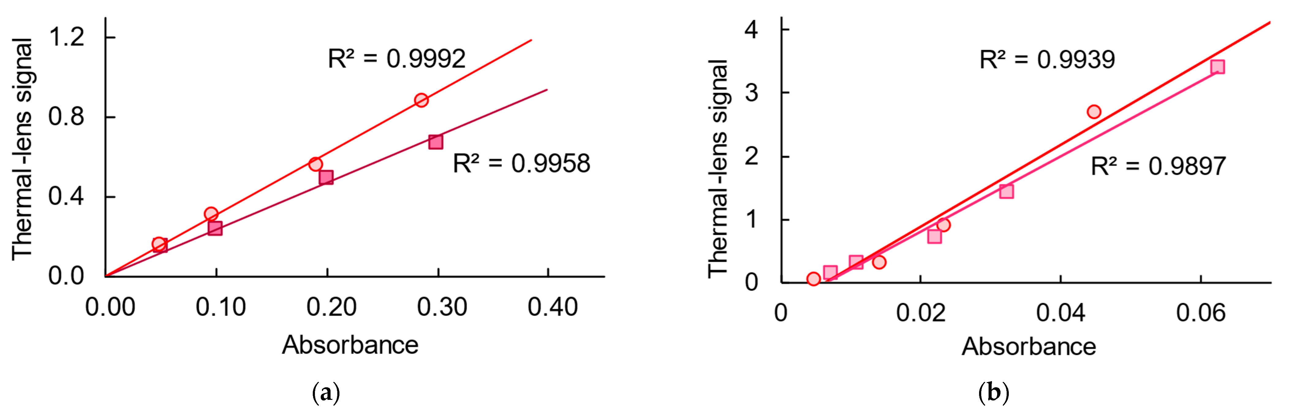
3.4. Steady-State Thermal-Lens Measurements

3.4.1. Hemoglobin

The determination of MetHbCN and ferroin shows low and similar LODs under moderate-power excitation conditions with the most sensitive setup TLS-60, as summarized in Table 2. The theoretical calculations of thermal-lens sensitivity for ferroin in water and various electrolyte solutions are in good agreement with the theoretical values from Equation (14) [122]. Compared to ferroin, the slope of the calibration plot of the thermal-lens signal vs. absorbance for MetHbCN in water is lower (Table 2 and Figure 4).

To prove that this effect results from the dispersive nature of MetHbCN solutions, we used mixtures of ferroin and MetHbCN; as the total thermal-lens signal is additive (as in photometry and Beer’s law), the slope should also be an additive function of the molarities of the components of such binary mixtures. For mixtures in 1.0 M PBS (Table 2), the experimental results are in good concordance with this hypothesis. The slope for a mixture can be predicted as $S_{\mathrm{mix}}={\eta }_{\mathrm{ferr}}{S}_{\mathrm{ferr}}+{\eta }_{\mathrm{MetHbCN}}{S}_{\mathrm{MetHbCN}}$, where S values are slopes for individual components, and η values are the molar fractions of ferroin and MetHbCN.

Measurements in saline solutions were intended, firstly, to show that a change in the environment leads to an increase in the sensitivity of the hemoglobin determination due to a change in thermophysical parameters [122] and, secondly, to find out how salts affect the signal linearity of the dispersed hemoglobin system. A mixture of sodium and potassium chlorides shows a significant increase in sensitivity, whereas phosphate solutions barely change the signal, and the mixture of four salts has the highest impact, which is not reducible to a mere sum of individual salt effects. Calibration dependences for MetHbCN and ferroin in 0.4 M KCl + 2.8 M NaCl are described by the following equations (P_e = 66.4 mW):

θ = (4.0 ± 0.1) × 10⁵c + (0.069 ± 0.004), (p = 0.95, n = 16, r = 0.988),

(24)

θ = (5.2 ± 0.1) × 10⁴c + (0.038 ± 0.002), (p = 0.95, n = 16, r = 0.996).

(25)

A comparison of the slopes of Equations (24) and (25) shows that there is a significant increase in the sensitivity of the determination of MetHbCN in saline media, and for ferroin, the sensitivity coefficient almost does not change compared to true solutions (Appendix C). The LOD of cyanmethemoglobin in saline media is 20 nmol/L (Table 2), which is 1.5 times lower than in the non-saline medium. The ferroin LOD does not change, which is consistent with the previous data for other saline solutions [122]. The ratio of sensitivity factors for cyanmethemoglobin and ferroin in a saline medium is 7.8 (Equations (24) and (25)), which agrees well with the value expected from the molar absorption coefficients. Thus, the influence of electrolytes is contrary to the thermal diffusion nature of such a difference in water [2], since thermal diffusion in electrolyte solutions should not be weaker than in distilled water. On the other hand, the effect of electrolytes on thermal conductivity and thermal effusivity is significant and may hide the weaker effect of dissolved chromophores. In general, the thermal-lens determination of cyanmethemoglobin in electrolyte solutions leads to a gain in the sensitivity coefficient and a decrease in detection limits.

3.4.2. Myoglobin

For myoglobin, the calibration slopes for TLS vs. transmission photometry (Equation (10)) for low powers of excitation are linear and barely change compared to ferroin as a true solution (Figure 4). For concentrations over 0.08% w/w, the concentration dependence of the thermal-lens signal depends on the excitation power in a more sophisticated way, and it changes from a nonlinear ascending curve to a curve with a maximum (Figure 5a) at excitation powers over 100 mW. The position of the maximum depends on the setup geometry, i.e., the excitation beam fluence, and somewhat corresponds to the nonlinear mode in photothermal microscopy [21,41,123]. With an increase in the excitation power, the range of signals for the same concentration range decreases (Figure 5b) and becomes very narrow for a power of 350 mW.

3.4.3. Bovine Serum Albumin

Albumins interact well with small molecules through electrostatic interactions. Thus, to change the properties of albumin, we used ferroin, which interacts well with this protein due to a pronounced positive charge, and the Cr(III) complex with EDTA (CrEDTA), which has a significantly lower charge density, i.e., it weakly interacts with albumin [124]. The modifying effect on the thermophysical parameters of albumin itself was estimated (Figure S3, Supplementary Materials). It shows a pronounced linear dependence on the concentration of albumin. At the wavelengths of excitation lasers, albumin does not absorb, which means that the signal increases mainly due to changes in thermal parameters.

In the presence of ferroin, there was an increase in the albumin concentration compared to albumin solutions, leading to a decrease in the slope of the calibration curves (Figure 6a). Moreover, the intersection of the calibration curves is in a narrow concentration range, proving that an increase in the ferroin concentration acts in the opposite direction to the albumin concentration. In the case of CrEDTA, we see linear dependences (Figure 6b) with the same slope.

The ratio of the slope for a given concentration of albumin, E_0,alb, to the slope in water, E_0,w, shows a different character for ferroin, for which it shows a constant decrease (Figure 7a), which depends on the ferroin concentration (Figure 7b). For CrEDTA, this relative slope is somewhat similar to the plots for myoglobin, with a small increase followed by a decrease in the value (compare Figure 5 and Figure 7). To further test albumin, we performed experiments with MetHbCN mixtures with albumin. For Hb concentrations corresponding to the middle of the calibration range (to decrease the overall error), the albumin addition (10–30 g/L) results in a decrease in the signal of more than 20% (Figure S4, Supplementary Information).

3.5. Transient Thermal-Lens Measurements

The transient curves for true solutions of ferroin and dispersed solutions of MetHbCN differ (Figure 8), and the characteristic times of thermal-lens measurements (Equation (5)) decrease significantly (Table 2). This behavior depends on the concentration (Figure 9a).

For MetHbCN and ferroin mixtures in saline solutions, the difference in characteristic time becomes smaller and even negligible (Figure 8b) compared to low ionic strengths. For myoglobin (Figure 8a), transient curves also differ from those of the ferroin solution, but the difference is much less compared to the same concentrations of MetHbCN, and the characteristic times of thermal-lens measurements (Equation (5)) decrease to a lesser degree than for hemoglobin for the same signals. The transient thermal-lens signal (Figure 8c) for albumin solutions does not show any significant deviations from the shape for most test concentrations; for 50 g/L in the presence of ferroin, a decrease in the relative probe intensity is revealed, which is much less than for heme proteins, as shown above.

For silica nanoparticles and nanodiamonds (Figure 10), transient curves expectedly differ from those of aqueous ferroin solutions, much more strongly compared to MetHbCN at the same absorption level, and the characteristic times of thermal-lens measurements (Equation (5)) decrease, which results from an increase in thermal diffusivity. As shown previously, for a dispersed system, the first part of the curve, up to approximately 10$t_c$, corresponds to the appearance of a system of nano-thermal-lenses around the nanoparticles, which results in an apparent increase in the thermal diffusivity [48,102], and at times over 40$t_c$, the course of the transient curve may be distorted due to thermal diffusion and convection. Thus, both light-absorption and thermophysical parameters were calculated for the range 10 ÷ 40$t_c$; the actual times differ for different setups.

The cooling (dissipation) curves of the thermal-lens measurements were taken separately from the heating curves due to the different behavior of these curves, as the signal development is governed by a balance between the external source fluence and the sample’s thermal properties, while dissipation depends on the stored energy and the solvent’s thermal effusivity. The curves for proteins showed little difference compared to water (Figure 11), and in all cases, the difference is lower than the error of the experiments and provides the same thermal diffusivity. To the contrary, the dissipation curves at high concentrations of silicon oxide nanoparticles (Figure 12) start to change with a steeper increase in the intensity due to the higher thermal diffusivities of these samples (Table 3).

4. Discussion

4.1. Back-Synchronized Detection Modality

In TLS, mode-mismatched two-beam (two-laser) schematics are dominant [2,4,31,49,50,125,126]. It requires separate beams: a beam inducing the photothermal effect (the excitation beam) and a beam that is distorted in the photothermal refractive-index field and then probed (the probe beam). The term ‘mode mismatching’ means that the waists of the focused beams are shifted relative to one another along the propagation axis, which provides the maximum probe sensitivity of the thermal-lens effect [127,128,129,130]. In photothermal microscopy, mode mismatching is necessary, as this technique provides the necessary sensitivity of measurements [3,13,35]. Even for confocal schematics, very slight mode mismatching is needed to provide the probe signal [22,41,131,132].

Unlike lock-in amplifier schematics, the data acquisition and processing system in the back-synchronized mode registers a thermal-lens signal that is directly calculated from the detected intensities of the probe beam Thus, it does not need an empirical conversion (amplification) factor as in lock-in schematics, which makes the thermal-lens signal value more meaningful, since it relies on the assessment and calculation of factors determined by the environment [100], e.g., molar absorptivities (Equation (3)). Thus, the sensitivity of thermal-lens measurements can be compared by using the absolute values of the signals from Equation (3), without involving the ratio of the signal of the test sample and some reference point, which is needed in most lock-in schematics [133,134,135,136].

Thermal-lens spectrometers for high-sensitivity measurements of light absorption usually have a tightly focused excitation beam (waist size of ca. 50–60 μm [14,86] or even less in micro-photothermal techniques [21,22,41,106,137,138,139,140,141,142]), which provides sufficient heating in the excited zone and, therefore, high optical detection sensitivity. However, such a schematic is not preferable for dispersed systems, especially when assessing the thermophysical parameters of the sample, because the heat flow from the heated zone depends on thermal conductivity, which may vary from the neat base solvents. Hence, the thermal-lens size becomes different for even a narrow concentration range, thus affecting the sensitivity and precision [2]. As a result, the geometry of the optical scheme for each sample should be changed to match the thermal lens and probe-beam sizes. Therefore, we designed spectrometers with a broad excitation beam (waist sizes, 150 and 300 μm), prolonging the time to attain a thermal equilibrium (Figure 1), and compared them to the more tightly focused beam in the ‘reference’ setup, TLS-60 (Table 1).

The main parameter of the generic optimization of the optical scheme in thermal lensing is the desired diameter of the excitation beam. This determines the spatial locality (the thermal element diameter) and the sensitivity (power density) [2,130,136,143]. Experimental and theoretical approaches for optimization result in the same conclusion [2,98]. Hence, all other parameters of the spectrometer (frequency) should be selected so that the thermal element diameter is approximately threefold larger than the excitation, and the probe-beam diameter should be equal to the bloomed thermal element diameter. This will give the most extended linear calibration range and the lowest LODs and LOQs [2].

Optimizing a thermal-lens spectrometer involves changing the interposition of the elements of the optical circuit of the thermal-lens spectrometer so that the size of the excitation beam does not change, and the probe beam passes through the entire heated region and includes three steps. This is necessary for the maximum accuracy and sensitivity of measurements. If the probe beam is wider than the heated zone, interference occurs between the part of the beam that does not pass through the solution and the part of the beam that is deflected when passing through the thermal lens (Figure 13a), resulting in noise in the signal, because of which the sensitivity decreases [2,144]. When the probe beam is too narrow (ca. several micrometers), the sensitivity drops because it passes only through a part of the heated region (Figure 13c). Thus, the maximum sensitivity is observed when the probe beam passes through the entire heated area (Figure 13b) [2,144].

The optimization of the optical scheme made it possible to achieve the constancy of the geometric parameter B for thermal-lens spectrometers. We achieved the maximum width of the linearity range of these dependences (Table 2). Thermal-lens spectrometers have been shown to work well with aqueous solutions and worse with organic media; this is due to the strength of the thermal-lens effect in non-polar solvents, which, for TLS-150, led to the quadratic dependence of the signal on the substance concentration, which is due to a change in the geometric parameters of the thermal lens and the deviation of the thermal-lens model (Equations (1)–(3) and (15)) with concentration [2,104]. There was also a decrease in the determination sensitivity for TLS-300 compared to TLS-150 due to beam broadening; however, this made it possible to work with toluene solutions, while TLS-150 does not allow this.

4.2. Transient and Steady-State Measurements

In addition to steady-state signals, which are mainly applied in thermal-lens measurements of light absorption or chemical analyses (concentration measurements), the cycle of the formation and dissipation of a thermal lens is characterized by periods of fall and increase in the intensity of the probe radiation (Figure 2), while transient thermal-lens signals are significantly more dependent on the thermophysical parameters of the medium than on light absorption (somewhat in contrast to steady-state signals) [2]. The transient thermal-lens curve depends on the thermal conductivity, heat capacity, thermal diffusivity, and dn/dT of the sample, absorption, and instrument geometry (Equation (3)). It should be noted that the difference in the transient development and dissipation curves of the thermal lens can be detected using the back-synchronized thermal-lens spectrometer because the thermal equilibrium is attained at every stage.

In true solutions, the absorbed energy is transformed after laser irradiation, which depends only on the energy distribution in the excitation beam. As a result, a gradient of the refractive index, the thermal lens, is formed. Due to the presence of large light-absorbing dispersed particles, part of the energy goes toward heating the particles themselves, and the heat transfer to the solution decreases, which leads to a noticeably weaker total thermal field in the sample irradiated by the laser [145]. Thus, for dispersed systems, the local heating at the beginning is located around particles with a high heat capacity, followed by the transfer of heat to the solvent, resulting in significantly more rapid heating and a reduction in the thermal-lens characteristic time. On the contrary, thermal-lens dissipation exhibits smaller changes compared to homogeneous samples because, for small temperature changes (10 mK, typical for the concentrations of most absorbing compounds in TLS), the dispersity of the medium provides a smaller impact on heat dissipation [2]. According to previous findings and models [41,96,108,146], this behavior (Figure 4, Figure 5 and Figure 6) is due to a higher heating rate near strongly light-absorbing dispersed particles, which, therefore, decrease the apparent thermal-lens characteristic time. Meanwhile, the heat transfer into the aqueous dispersion is slower [93,108], which leads to more heat dissipation during the development (blooming) of the thermal lens. The average distance between the globules for this concentration range is 30–300 nm, comparable to the Hb globule size, and should affect the thermal properties. If the absorbance of solutions is the same, this effect decreases the steady-state thermal-lens signal from a dispersed system compared to a true solution without a linearity loss (Figure 4).

4.3. Measurement Conditions

The microheterogeneity of the medium, e.g., the presence of a surfactant in an aqueous solution, usually increases the thermal-lens signal, and with an increase in its concentration, the signal expectedly increases due to changes in thermal parameters [147,148,149]. However, special attention should be paid to the conditions (excitation power and time selection) of a thermal-lens experiment in dispersed media, particularly for steady-state (stationary) measurements [84,97,150]. Firstly, in two-component media, the role of the temperature gradient in the solution is twofold. It forms both a refractive-index profile (the thermal lens) and a concentration profile of solute molecules in solution due to thermal diffusion (thermodiffusion, the Soret effect) [28,151,152,153]. This concentration spatial profile may function as another lens-like optical element contributing to probe-beam blooming, together with the thermal-lens action. Thus, the signal (positive or negative) due to the Soret effect may mistakenly be interpreted as an increase or decrease in the thermal-lens signal, which may lead to errors in assessing a light-absorbing analyte [2]. To separate the effects of temperature and concentration gradients, it is necessary to use special techniques, e.g., time selection of the signal [28,154], or the settings of the parameters to efficiently evaluate and exclude the accompanying thermally induced diffusion processes.

Secondly, thermal-lens experiments are accompanied by convective heat transfer, which decreases the thermal-lens strength and disturbs the photothermal effect, with periodic fluctuations resulting in increased measurement errors, i.e., both bias and random errors of photothermal measurements [155,156,157,158]. The periodic nature of thermal-lens measurements facilitates convection and provides the possibility of studying convective phenomena. However, in most tasks of thermal-lens measurements (thermophysical or light-absorption/concentration parameters), convection is a degradation factor for both accuracy and precision, and it should be suppressed if possible. Back-synchronized thermal lensing, by default, uses different times for steady-state heating, and full dissipation usually suppresses convective effects in thermal lensing.

Thus, time selection in thermal lensing is of prime importance because we need to select the time of blooming and the dissipation of the thermal lens to provide (i) the maximum sensitivity of the thermal-lens effect and (ii) the maximum accuracy and precision of the measurements. The second problem depends on the information we need to obtain from the experiments: thermal diffusivity requires short times and the analysis of the transient curves, while absorption measurements require steady-state measurements.

It is worth mentioning that as the thermal-lens effect is scaled depending on the fluence (and the excitation beam size) and thermal diffusivity of the base medium, the characteristic time (Equation (5)) is a scale parameter for time selection. Thus, to generalize the problem, it is expedient to use the relative time scale of measurements, i.e., $t/t_c$ values (Figure 14). Using the example of the most narrowly focused TLS-60 setup (characteristic time in water is 6.1 ms, Table 2), Figure 14 (a single, non-averaged curve to more explicitly show the changing error) shows that in time curves in the interval of steady-state measurements of the heating part (Figure 2), the time $\left(0.5÷5\right)\times t_c$ corresponds to the transient process (marked by the yellow rectangle), and $(5÷20)\times t_c$ corresponds to approaching the steady state (the green rectangle). Longer times correspond to steady-state measurements, and $t_1+t_2=\left(20÷40\right)\times t_c$ provides steady-state measurements with the minimum error, while at longer values (the red rectangle), some other effects start to appear (the Soret effect). As a result, up to 20t_c (ca. 125 ms), the curves for water reasonably fit the theoretical equation (Equation (3)). At 100 ms, the time curves approach the plateau, which is in good concordance with the theory.

It should be noted that $t_c$ is the heating characteristic time, and it could be used to characterize the dissipation curve with caution. The physical meaning of $t_c$, the half-blooming of the probe beam, is the relative decrease in intensity, which is 0.5 (Figure 2) compared to the steady state. In the cooling half-cycle, the relative decrease in intensity of 0.5 has no such meaning (Figure 14). However, as $t_c$ is the generic time scale of a thermal-lens experiment, the normalized time scale seems appropriate for characterizing the dissipation of the thermal lens. Thus, for the cooling period of the excitation on/off cycle, the transient period is the same as for the heating period, $\left(0.5÷7\right)t_c$, and the period of approaching the steady state is longer, (7$÷30)t_c$. The steady state can be measured in the time interval $t_3+t_4=\left(30÷50\right)t_c$ or for even longer times.

However, the accuracy of measurements may be affected by the deviation of the transient curve from Equation (3) in dispersed media due to the nanolens formation at early stages [106]. Thus, for nanodiamonds and colloidal silica particles (Figure 10), a steeper decrease in the relative probe-beam intensity means decreasing the apparent characteristic time. However, the direct application of Equation (5) for the calculation of thermal diffusivity would result in an overestimation. As a result, the straightforward use of the linear part of the cooling transient curve at $\left(0.5÷10\right)t_c$ for dispersed media seems incorrect due to a positive bias, and the use of longer times seems more expedient. However, long times may result in the appearance of conductive and convective heat transfer [158] and also seem inexpedient. Thus, the time selected for data handling depends on the task: for light-absorption parameters, the plateaus should be selected with the maximum number of points to decrease the error, while for thermal parameters, the early stages corresponding to nanolens formation in dispersed media [106] should be excluded, as well as long heating times, which may involve conductive and convective heat transfer as well as thermal diffusion effects.

4.3.1. Reproducibility and Replicability

The first precision parameter is reproducibility, which, according to ISO 5725-1, specifies the closeness of agreement between independent test results obtained with the same method on identical test material but under different conditions (different apparatuses, different operators and laboratories, and a considerable time interval between measurements). Previously, we showed that the reproducibility of thermal-lens measurements in true solutions [111], aqueous surfactant solutions [159], and polymer-unmodified aqueous solutions [97] does not differ from that in pure water and mainly depends on the error in sample preparation procedures. This is supported by other findings in thermal lensing [11,88,101,160] and photothermal-lens microscopy [11,91,161,162].

A significant difference between the components of the root-mean-square deviations of replicability (Equation (22)) and reproducibility (Equation (23)) confirms our previous findings [100] that the main contribution to the error is from reproducibility (procedures and protocols for sample preparation), while the repeatability precision of thermal-lens measurements is almost independent of the test substance and its concentration and depends on the thermal-lens setup only and its instrumental optimization. For proteins, the experimental curve seems to fit the theoretical prediction well (Equation (23)).

4.3.2. Repeatability

Another precision factor is repeatability, which, according to ISO 5725-1, specifies the closeness between results obtained under the same experimental conditions (the same operator, laboratory, and apparatus, with a short interval between measurements). This characteristic is less significant in a chemical analysis in biomedical studies because it mainly characterizes an instrumental (meter) error.

In thermal-lens spectrometry, this parameter is represented by short-term fluctuations of the signal from excitation on/off cycles. The contribution to the repeatability RSD from the instrument error (laser power fluctuations and jitter of optical elements) is significant but is much lower than the solvent effect (Equations (3) and (9)). The most curious fact is that RSD in some solvents depends much less on the sample absorbance or the excitation power in some signal ranges [93,111]. In other words, a statistical parameter acquires the meaning of the thermo-optical constant of the sample, or at least of a signature parameter. Repeatability depends on thermal diffusivity, non-equilibrium heat transfer (including nanolens formation), convection, and the Soret effect. Still, the separate contributions of thermophysical processes are difficult to find directly. Therefore, a repeatability comparison for two samples (all other conditions being the same) provides the estimation for thermal-lens detection limits and sensitivity coefficients, and this works for different solvents and additives in solutions [163].

Here, we considered repeatability parameters for the studied proteins and nanoparticle solutions. For pure water with inert colorants, RSD_rep (Equation (21)) vs. the steady-state thermal-lens signal (Equation (7)) (Figure 15a) is similar to the low-absorption branch of the reproducibility curve (Figure S1, Supplementary Materials [101]), as the instrumental meter error decreases with an increase in the light absorption for absorbances low enough to ensure no significant deviation from the thermal-lens model [2,104,164,165]. For proteins, the actual values increase (Figure 15a), probably due to a change in the size of the thermal lens in these media. Such independence of the relative standard deviation from the concentration (Figure 15a) was also found for surfactants of various origins within the range 1–10 mmol/L. This is in good agreement with the existing data showing that, for these concentrations of nonionic surfactants, the water structure is not significantly changed owing to insignificant changes in the hydrogen-bond structure [147].

However, as surfactants affect the thermal properties of water much more, the following changes in RSD_rep curves for nonionic surfactants and SDS most likely result from a change in the thermal properties of the aqueous solution caused by an increase in the number of micelles rather than in their size. The growth of fluctuations for higher surfactant concentrations (over 100 mmol/L) is probably caused by the increasing non-homogeneity of dispersed solutions and the contribution of light scattering, which can be accounted for by a change in the micelle shape from spherical to cylindrical as well as their aggregation [166]. In Triton X-100, fluctuations grow and reach a plateau at 7 mmol/L. Then, in the range of 0.007–0.15 mol/L Triton X-100, the fluctuations are twofold higher than in pure water (20–25%). For Brij-35, the fluctuations are virtually constant up to 50 mmol/L (Figure 15a) and start increasing again with a further increase in the surfactant concentration. Thus, the effect of surfactants on the thermal-lens repeatability in aqueous media differs significantly from that of non-surfactant substances and should be taken into account, e.g., when inert modifiers are used along with proteins in light-absorption measurements [99].

It is worth mentioning that dispersed phases also affect the thermal-lens measurements and can be used not only as a measure of thermal properties but also as the signal source. The interference from poorly soluble compounds of metals on the thermal-lens determination of bismuth [167] manifests itself in the relative standard deviation of the reagent mixture (blank) and the analyte signals (Figure 15b). The blank signal does not depend on the concentrations of certain amounts of other metals (without bismuth), and RSD_rep also does not change, which is shown as the horizontal parts of the curves in a rather broad range of the molar ratios of the interferent metal and bismuth ions. However, starting from a certain concentration of the interferent metal, RSD_rep is increased by a factor of 2–20, as represented by the increasing parts of the curves (Figure 15b). The metal concentrations corresponding to this increase in RSD_rep are much higher than the solubility constants of corresponding iodides or oxides that can form under these conditions [168]. Thus, it could be said that the thermal-lens effect reacts to the formation of rather finely dispersed solutions of these species. This is confirmed by a gradual increase in RSD_rep prior to changes in the thermal-lens signal in the monitoring of spontaneous precipitation [169]. Despite multiple manifestations of this effect in thermal-lens experiments, its description is still qualitative, and its use is limited. The differences in RSD_rep for proteins found in this study are slight compared to true solutions of model systems, which made it impossible to use them for characterization. Still, the use of RSD_rep as a signature parameter in thermal-lens studies seems relevant for the further development of the method.

Most previous studies estimated the repeatability of steady-state measurements of lock-in measurements with a time constant. In this study, we estimated RSD_rep for transient measurements as a function of the transient thermal-lens signal (Equation (3)). By deconvoluting a transient thermal-lens curve, it is possible to describe the thermal equilibrium and to assess the early stages of thermal-lens development that may depend more on the dispersed-phase parameters. As expected, the data corresponding to approaching the thermal equilibrium (Figure 14) show the same good precision as steady-state signals, while the estimation of RSD_rep for earlier stages ($0.5÷10\times t_c$) did not show any valuable data.

4.4. Hemoglobin and Myoglobin

Changes in the characteristic time $t_c$ for hemoglobin solutions (Figure 8 and Figure 9) compared to true solutions are more distinct than changes in the slope of a concentration calibration (Figure 4) and are comparable to those for nanoparticle solutions (Figure 10). The characteristic time in MetHbCN solutions depends on the protein concentration (Figure 9); the $t_c$ value for ferroin–MetHbCN mixtures is additive (Table 2 and Figure 9b). An equimolar mixture of MetHbCN and ferroin shows a shift in $t_c$, as expected from component molar fractions. This model for thermal lensing in MetHbCN solutions is well simulated by applying the multipoint heat-source theoretical approach (Appendix B) [95,96,108]. This effect of Hb globules with high local light absorption (compared to the much less absorbing solution around them) is responsible for local hot zones previously reported for RBCs [170,171].

The approach based on thermal-lens development as an ensemble of point sources predicts this in a semiquantitative way [95,96]; however, a full solution requires further developments in theory. Moreover, apart from the change in the conductive heat-transfer mechanism in dispersed solutions, such a significant difference in the sensitivity coefficient and characteristic time can result from convection heat transfer [143,158,172,173] and the Soret effect [28,151,152,153]. However, in such cases, the transient curves would be poorly described by the mono-exponential dependence characteristic of a purely thermal-lens effect and described much better by bi-exponential dependences corresponding to concurrent conductive and convective or thermal and concentration lenses.

If the hypothesis about the influence of dissolved hemoglobin on the thermophysical properties of the medium is correct, then the development and dissipation curves of the thermal lens should remain close to mono-exponential, but the characteristic times of the development of the thermal lens should differ from those of a purely aqueous medium, as discussed above. In addition, the characteristic time of thermal-lens development and dissipation should differ to a greater extent than in a water environment due to the different effects of the solute (in this case, hemoglobin) on the thermal conductivity and thermal effusivity of the medium. To verify this, transient development curves of the thermal-lens signal were recorded at different concentrations of MetHbCN, ferroin, and their mixtures in aqueous and saline media (Figure 8 and Figure 9). Based on the selection of measurement parameters (Section 4.3), we ensure the achievement of a stationary thermal state.

For thermal-lens heating and cooling curves, the functions y = ae^−bx and y = a(1 – e^−bx), respectively, gave the worst approximations, with correlation coefficients less than 0.7 in all cases, so they were not used further. For other functions, y = y₀ + ae^−bx for a purely thermal-lens effect and y = y₀ + ae^−bx + fe^−gx, representing two competitive mechanisms, the correlation coefficients were not lower than 0.97 (Table S2, Supplementary Materials). Thus, the thermal-lens development curve is well described by a shifted mono-exponent. It indicates a weak Soret effect or a slight contribution from convective heat transfer to the transient signal under the selected measurement conditions and test samples.

The medium changes when adding electrolytes that affect the sensitivity (Table 2). As expected, the slope changes for ferroin follow the electrolyte thermal diffusivity and the temperature gradient of the refractive index [122]. However, the changes in the calibration slope for MetHbCN are more drastic and do not directly depend on the ionic strength but rather on the electrolyte nature, with an additional increase in PBS compared to chloride solutions only (Table 2). Additionally, for higher ionic strengths, the difference in the thermal-lens characteristic time between true solutions and protein dispersions becomes smaller and even negligible (Figure 8), and the error in the estimation of changes in the characteristic time using Equation (5) increases significantly. The multipoint response calculation (Appendix B) results in a smooth spatial profile with a higher temperature in the beam center, which correlates entirely with the increase in the slope and characteristic time for MetHbCN (Table 2). Thus, transient curves and characteristic times for various electrolyte-based media containing MetHbCN showed concordance with a decrease in the slope of the calibration θ = f(A) (Equation (10)) responsible for bulk thermal properties and is in good concordance with the result of a multipoint light-absorbing model of thermal-lens measurements [96,108].

A comparison of the slopes of the curves shows a significant increase in the sensitivity of the determination of MetHbCN in saline media, and for ferroin, the sensitivity coefficient barely changes. The detection limit of MetHbCN in the saline medium is 20 nmol/L (Table 2), which is 1.5 times lower than in the non-saline medium. The ferroin detection limit does not change, which is consistent with previous data for other saline media [122]. The ratio of sensitivity factors for both MetHbCN and ferroin in the case of a saline medium is 7.8, which agrees well with the value expected from the molar absorptivities for these substances. Thus, the impact of electrolytes eliminates the difference between the development of the thermal-lens effect for MetHbCN and ferroin, which is contrary to the thermal diffusion nature of such a difference [2], since thermal diffusion in electrolyte solutions should be no weaker than in distilled water. On the other hand, the effect of electrolytes on the parameters of the medium (thermal conductivity and thermal effusivity) is significant and may hide the weaker effect of dissolved chromophores. In general, the thermal-lens determination of MetHbCN in electrolyte solutions leads to a gain in the sensitivity coefficient and a favorable decrease in detection limits.

In the case of myoglobin, all of the effects discussed in the previous section for hemoglobin are much less pronounced (Figure 8 for transient and Figure 4 for steady-state measurements). This correlates well with the point-source approach’s profile calculation. Very characteristic is the slope dependence and the whole behavior of the concentration dependence of myoglobin on laser power (Figure 5), which shows that local overheating due to nanolens formation depends on the power and fluence. This behavior is remarkably similar to the local overheating and so-called nonlinear mode in photothermal microscopy [21,41,123]. In the latter case, it is due to the formation of nanobubbles in hot zones around the nanostructures, which increases the sensitivity of imaging and quantification. In our case of a rather slow thermal-lens effect and steady-state thermal lensing, the result is quite the opposite: a decrease in the sensitivity down to a decrease in the signal with the chromophore concentration. In our opinion, such behavior can be readily seen with myoglobin, as it allows high excitation powers to be used with no decomposition of this protein.

4.5. Bovine Serum Albumin

Contrary to heme proteins, the transient thermal-lens signal for albumin solutions (Figure 8c) does not show any significant deviations in either the shape or the characteristic time. It confirms the absence of thermal diffusion in the solution, which further confirms the thermal character, rather than being concentration-based, of the signal decrease in this case. Figure S3 (Supplementary Information) shows the pronounced linear dependence of the signal on the albumin concentration. Such an increase in the signal of aqueous albumin solutions shows its modifying effect on the thermal parameters. Spectrophotometric measurements showed that in the selected wavelength range, albumin does not absorb, which means that the signal increases due to the photothermal parameters of the solution.

Experiments with ferroin and CrEDTA chelate were used to further prove the effects of point-source absorption on the response of the system under photothermal heating. Ferroin, which, as expected, interacts with albumin to a much higher degree than CrEDTA, is similar to hemoglobin: light-absorbing nanostructures (albumin with ferroin) in a non-absorbing medium. While albumin itself does not absorb at the excitation wavelength and thus cannot be a heat source, the ferroin–albumin complex leads to the formation of light-absorbing point sources that transfer less heat to the solution compared to aqueous ferroin, and it leads to local overheating. Thus, from the viewpoint of light absorption and photothermal heating, we have a dispersed medium with excess ferroin, with a part of it, upon interaction, being attached to albumin globules. Thus, we have almost the same situation as with MetHbCN, where some of the light-absorption centers are point heat sources in photothermal heating. Thus, the more albumin added (Figure 7a), the greater the fraction of light absorption of point heat sources, and the lower the final signal. If we consider the ferroin concentration, we have a confirmation of this: the higher the ferroin concentration (more point heat sources formed), the steeper the slope (Figure 7b), while the total signal increases due to the higher total absorption of ferroin.

In the case of the CrEDTA complex with a weaker interaction between albumin and CrEDTA, the calibration slopes (Figure 6b) do not differ significantly from an unmodified aqueous medium. However, in general, it has a similar behavior (Figure 7a) to myoglobin (Figure 5). This is due to competitive effects: an increase in the signal due to changes in the thermal parameters of the solution upon an increase in the albumin concentration and a decrease in the signal due to point sources on the transient curves. As the point-source effect is much slower, it is manifested as a lower decrease compared to ferroin and at higher concentrations. As a proof-of-concept, we used samples of albumin with cyanmethemoglobin. These proteins can interact, forming a larger nanostructure [174]. Thus, this effect should be revealed in thermal lensing under selected conditions. As in previous cases, photometric measurements did not show a significant change in absorbance between MetHbCN and MetHbCN/albumin solutions. However, thermal lensing shows a ca. 20% decrease compared to MetHbCN (Figure S4, Supplementary Information), which is higher than the effect of ferroin/albumin mixtures. Within the framework of this study, this was intended as a demonstration experiment, which proved the interaction effect on thermal lensing, and further studies are needed for a more detailed description.

4.6. Comparison with Engineered Nanoparticles

Thus, heating curves for all of the studied proteins show changes compared to aqueous solutions without proteins, while dissipation curves show much smaller changes in their behavior compared to heating curves (compare Figure 11 vs. Figure 8 and Figure 9). This is accounted for by a very slight change in the thermal diffusivity of aqueous protein solutions compared to solutions of nanoparticles and fullerene/nanodiamond aggregate structures (Figure 11), which, in the case of silica nanoparticles, are heat-conducting nanofluids (Table 3). This effect ensures more profound nanolens-driven transient curves for nanoparticles. For nanodiamonds, the heating curves seem to show the same situation, lowering t_c with the nanoparticle concentration. However, as we have shown previously [106,119], nanodiamonds are rather poor heat-conducting nanofluids, as photothermal heating accumulates the heat during the heating period of the photothermal-excitation cycle. This results in the reversed behavior of the cooling curve (Figure 11): the dissipation becomes slower due to the action of secondary heating sources. Thus, the cooling curve for a colloidal solution cannot be approximated by the classical temperature equation for a homogeneous medium (Equation (18)), which is experimentally confirmed in the case of water. As the studied protein solutions show overheating and no changes in cooling curves, this shows their somewhat insignificant effect on thermal parameters.

The whole comparison of the results for all three studied proteins and nanoparticle systems allows us to make the following methodological conclusions for measurements in dispersed media. First, tests for accuracy and precision with true and dispersed solutions are demonstrated with known protocols of production (gold, silver, or silica). As protein solution properties may vary due to reaction conditions, prior to thermal lensing, calibration with nanoparticles with different but well-established properties should be performed. In our opinion, the silica nanoparticles used in this study or metal or metal-oxide particles forming heat-conducting nanofluids can be used for this purpose. The advantage of metal or oxide nanoparticles is the possibility of obtaining thermal diffusivity or thermal effusivity values from alternative methods [106,119]. The use of nanodiamonds as calibration samples seems inexpedient due to various properties depending on the nanodiamond brand and the uncommon behavior of the cooling curve [106,107,143,145]. Certainly, if a more precise model for the thermal properties of aqueous dispersions of nanodiamonds (as heat-conducting and simultaneously heat-accumulating solutions) is presented, nanodiamonds can be used as well. Contrary to nanodiamonds, fullerenes may be an expedient candidate for calibration, as they mildly alter the bulk thermal properties compared to nanofluids, and their nanostructural parameters in solution change from true to slightly heat-conducting aggregates depending on the solvent and environment [107,143,145].

5. Conclusions

This study shows that transient and steady-state thermal lensing should not be performed alone for samples with unknown absorption/concentration and thermal properties, and they should be used together. This study shows that the simultaneous estimation of thermal and optical/concentration parameters of dispersed systems should provide (i) the maximum sensitivity of the thermal-lens effect (absorption measurements) and (ii) the maximum accuracy as well as precision of the measurements (thermal parameters). Thus, time selection for thermal lensing (stages of transient blooming, transient dissipation, and steady states) becomes the key stage, as assessing thermal diffusivity requires the analysis of transient curves and relatively short excitation times, while absorption parameters necessitate steady-state measurements with longer times and prolonged signal accumulation. Therefore, the time scale (thermal-lens characteristic time, $t_c$) should be selected at the stage of the thermal-lens setup design, and the relative time intervals should be selected: $\left(0.5÷5\right)t_c$ for transient and (5$÷20)t_c$ for steady-state measurements. These estimations can be treated as generic for aqueous dispersed systems, as various substances were used (proteins, surfactants, inorganic iodides, and silica oxide and carbon nanoparticles). Still, these parameters should be studied for other dispersed systems and base solvents.

Thus, a thermal-lens spectrometer for dispersed solutions could be implemented as a multifunctional apparatus upon the selection of measurement parameters governed by both accuracy and precision. The balance between the precision of measurements of thermal and optical parameters corresponds to excitation beam sizes of 60–300 µm; a broad excitation beam provides longer times to attain a thermal equilibrium and, thus, the better precision of measurements of thermal diffusivity, though increasing the measurement time and decreasing the accuracy of steady-state measurements. The setups fabricated in this study provide good balance and flexibility for both measuring light-absorption parameters and assessing the concentrations of dispersed solutions with trace levels of constituents and assessing the thermal properties of dispersions. Despite a decrease in the sensitivity of light-absorption measurements of lock-in schematics, the setups retain the features of the sensitivity and instrumental/data-handling simplicity of common dual-beam thermal lensing. In our opinion, an important feature of the back-synchronized schematics used in this study is the possibility of selecting and monitoring both the accuracy and precision of measurements depending on the sample and task (thermal or light-absorption properties). Apart from the multi-signal feature, these joint measurements enable the separation of thermal and concentration parameters and should be accompanied, if possible, by the assessment of either light-absorption or thermophysical properties using other methods.

The obvious disadvantage of conventional thermal lensing is that the thermal-lens effect is ensemble-based, not molecule/structure-based, and non-microscopic measurements always provide the bulk properties of the sample. Still, the very large volume of information from transient thermal lensing simultaneously with the information channel from steady-state measurements provides a way to obtain rather valuable information. For instance, in the case of albumin interaction, thermal lensing can be used for screening various conditions or classifying the interactions by signature effects before more detailed experiments are performed. This feature of thermal lensing can be implemented even in a handheld device for rapid tests of complex samples alongside or before photothermal-microscopy, light-scattering, or fluorescence measurements. Such an experimental design can be extended to pulsed thermal-lens excitation conditions [52,175,176,177,178,179,180] not considered here. In that case, short excitation times close to or shorter than the thermal-lens characteristic times may increase the sensitivity due to the more substantial overheating of such entities as Hb globules, mitochondria, etc., and reveal features that are hidden or averaged at the early stages of signal development in the cw excitation conditions used in this study. It may provide, e.g., a means of estimation of the protein globule size in solution, which is beyond the abilities of the setups built in this study due to an insignificant contribution of individual nanolens entities (light-absorbing point sources) in bulk cw thermal lensing.

Certainly, these experiments may (and should) be combined with photothermal microscopic techniques, especially for transient measurements. Transient thermal lensing can overcome the diffraction limit of optical photothermal spectroscopy [41,181,182] to attain the super-resolution of photothermal imaging, which is highly important for various applications, such as studies of mitochondria, erythrocyte pathologies, and similar problems [146,181]. The following studies should integrate all photothermal measurements into a single compact device for micro-measurements [43].

Finally, despite the relatively reliable estimations attained in this study, a theory that combines the size and the nature of dispersed particles and the whole quantitative picture of the thermal-lens effect is not fully developed, and only the estimation of the range of the particle/aggregate/cluster size can be performed; addressing this could be the aim of advanced research in this direction.

References

1. Dy, E.; Gu, C.; Shen, J.; Qu, W.; Xie, Z.; Wang, X.; Baesso, M.L.; Astrath, N.G.C. Sensitivity enhancement of thermal lens spectrometry. J. Appl. Phys. 2022, 131, 063102. [Google Scholar] [CrossRef]
2. Bialkowski, S.E.; Astrath, N.G.C.; Proskurnin, M.A. Photothermal Spectroscopy Methods; Wiley: Hoboken, NJ, USA, 2019; p. 512. [Google Scholar]
3. Mawatari, K.; Ohashi, T.; Ebata, T.; Tokeshi, M.; Kitamori, T. Thermal lens detection device. Lab Chip 2011, 11, 2990–2993. [Google Scholar] [CrossRef] [PubMed]
4. Proskurnin, M.A.; Khabibullin, V.R.; Usoltseva, L.O.; Vyrko, E.A.; Mikheev, I.V.; Volkov, D.S. Photothermal and optoacoustic spectroscopy: State of the art and prospects. Phys.-Uspekhi 2022, 65, 270–312. [Google Scholar] [CrossRef]
5. Liu, M. Influence of thermal conductivity on photothermal lens spectroscopy. Thermochim. Acta 2019, 672, 126–132. [Google Scholar] [CrossRef]
6. Dada, O.O.; Feist, P.E.; Dovichi, N.J. Thermal diffusivity imaging with the thermal lens microscope. Appl. Opt. 2011, 50, 6336–6342. [Google Scholar] [CrossRef] [PubMed]
7. Constantino, R.; Lenzi, G.G.; Franco, M.G.; Lenzi, E.K.; Bento, A.C.; Astrath, N.G.C.; Malacarne, L.C.; Baesso, M.L. Thermal Lens Temperature Scanning technique for evaluation of oxidative stability and time of transesterification during biodiesel synthesis. Fuel 2017, 202, 78–84. [Google Scholar] [CrossRef]
8. Yamaoka, S.; Kataoka, Y.; Kazama, Y.; Fujii, Y.; Hibara, A. Efficient thermal lens nanoparticle detection in a flow-focusing microfluidic device. Sens. Actuat. B 2016, 228, 581–586. [Google Scholar] [CrossRef]
9. Martelanc, M.; Ziberna, L.; Passamonti, S.; Franko, M. Application of high-performance liquid chromatography combined with ultra-sensitive thermal lens spectrometric detection for simultaneous biliverdin and bilirubin assessment at trace levels in human serum. Talanta 2016, 154, 92–98. [Google Scholar] [CrossRef] [PubMed]
10. Franko, M.; Liu, M.; Boskin, A.; Delneri, A.; Proskurnin, M.A. Fast Screening Techniques for Neurotoxigenic Substances and Other Toxicants and Pollutants Based on Thermal Lensing and Microfluidic Chips. Anal. Sci. 2016, 32, 23–30. [Google Scholar] [CrossRef] [Green Version]
11. Liu, M.; Franko, M. Progress in thermal lens spectrometry and its applications in microscale analytical devices. Crit. Rev. Anal. Chem. 2014, 44, 328–353. [Google Scholar] [CrossRef]
12. Cabrera, H.; Goljat, L.; Korte, D.; Marin, E.; Franko, M. A multi-thermal-lens approach to evaluation of multi-pass probe beam configuration in thermal lens spectrometry. Anal. Chim. Acta 2020, 1100, 182–190. [Google Scholar] [CrossRef] [PubMed]
13. Fujii, N.; Harata, A. Development of Reflection Objective-Employed Collinear Mode-mismatched Thermal Lens Microscope. Jpn. J. Appl. Phys. 2011, 50, 07HC05. [Google Scholar] [CrossRef]
14. Proskurnin, M.A.; Volkov, D.S.; Gor’kova, T.A.; Bendrysheva, S.N.; Smirnova, A.P.; Nedosekin, D.A. Advances in thermal lens spectrometry. J. Anal. Chem. 2015, 70, 249–276. [Google Scholar] [CrossRef]
15. Abelha, T.F.; Calvo-Castro, J.; Lima, S.M.; Silva, J.R.; da Cunha Andrade, L.H.; de Mello, J.C.; Dreiss, C.A.; Green, M.; Dailey, L.A. Thermal Lens Spectrometry Reveals Thermo-Optical Property Tuning of Conjugated Polymer Nanoparticles Prepared by Microfluidics. ACS Appl. Polym. Mater. 2022, 4, 6219–6228. [Google Scholar] [CrossRef]
16. Liu, M.Q.; Franko, M. Thermal Lens Spectrometry: Still a Technique on the Horizon? Int. J. Thermophys. 2016, 37, 1–16. [Google Scholar] [CrossRef]
17. Liu, M.; Korte, D.; Franko, M. Theoretical description of thermal lens spectrometry in micro space. J. Appl. Phys. 2012, 111, 033109. [Google Scholar] [CrossRef]
18. Liu, M.; Franko, M. Theoretical Analysis for Sensitivity Enhancement in Broad-band Thermal Lens Microscope. Adv. Mater. Res. 2012, 503, 1480–1483. [Google Scholar] [CrossRef]
19. Fischer, M.; Georges, J. Sources of errors in the use of calorimetric references for photothermal spectroscopic methods. Anal. Chim. Acta 1996, 334, 337–344. [Google Scholar] [CrossRef]
20. Marcano, A.O.; Delima, F.; Markushin, Y.; Melikechi, N. Determination of linear and nonlinear absorption of metallic colloids using photothermal lens spectrometry. J. Opt. Soc. Am. B 2011, 28, 281–287. [Google Scholar] [CrossRef]
21. Nedosekin, D.A.; Galanzha, E.I.; Dervishi, E.; Biris, A.S.; Zharov, V.P. Super-Resolution Nonlinear Photothermal Microscopy. Small 2014, 10, 135–142. [Google Scholar] [CrossRef]
22. Nedosekin, D.A.; Foster, S.; Nima, Z.A.; Biris, A.S.; Galanzha, E.I.; Zharov, V.P. Photothermal confocal multicolor microscopy of nanoparticles and nanodrugs in live cells. Drug Metab. Rev. 2015, 47, 346–355. [Google Scholar] [CrossRef] [Green Version]
23. Zong, H.; Yurdakul, C.; Bai, Y.; Zhang, M.; Ünlü, M.S.; Cheng, J.-X. Background-Suppressed High-Throughput Mid-Infrared Photothermal Microscopy via Pupil Engineering. ACS Photonics 2021, 8, 3323–3336. [Google Scholar] [CrossRef] [PubMed]
24. Adhikari, S.; Spaeth, P.; Kar, A.; Baaske, M.D.; Khatua, S.; Orrit, M. Photothermal Microscopy: Imaging the Optical Absorption of Single Nanoparticles and Single Molecules. ACS Nano 2020, 14, 16414–16445. [Google Scholar] [CrossRef] [PubMed]
25. Zeng, Z.-C.; Wang, H.; Johns, P.; Hartland, G.V.; Schultz, Z.D. Photothermal Microscopy of Coupled Nanostructures and the Impact of Nanoscale Heating in Surface-Enhanced Raman Spectroscopy. J. Phys. Chem. C 2017, 121, 11623–11631. [Google Scholar] [CrossRef]
26. Georges, J. Advantages and limitations of thermal lens spectrometry over conventional spectrophotometry for absorbance measurements. Talanta 1999, 48, 501–509. [Google Scholar] [CrossRef] [PubMed]
27. Marcano, A.; Alvarado, S.; Meng, J.; Caballero, D.; Moares, E.M.; Edziah, R. White Light Photothermal Lens Spectrophotometer for the Determination of Absorption in Scattering Samples. Appl. Spectrosc. 2014, 68, 680–685. [Google Scholar] [CrossRef]
28. Georges, J. Matrix effects in thermal lens spectrometry: Influence of salts, surfactants, polymers and solvent mixtures. Spectrochim. Acta. A Mol. Biomol. Spectrosc. 2008, 69, 1063–1072. [Google Scholar] [CrossRef]
29. Luna-Sánchez, J.L.; Jiménez-Pérez, J.L.; Carbajal-Valdez, R.; Lopez-Gamboa, G.; Pérez-González, M.; Correa-Pacheco, Z.N. Green synthesis of silver nanoparticles using Jalapeño Chili extract and thermal lens study of acrylic resin nanocomposites. Thermochim. Acta 2019, 678, 178314. [Google Scholar] [CrossRef]
30. Deus, W.B.; Ventura, M.; Silva, J.R.; Andrade, L.H.C.; Catunda, T.; Lima, S.M. Monitoring of the ester production by near-near infrared thermal lens spectroscopy. Fuel 2019, 253, 1090–1096. [Google Scholar] [CrossRef]
31. Ventura, M.; Deus, W.B.; Silva, J.R.; Andrade, L.H.C.; Catunda, T.; Lima, S.M. Determination of the biodiesel content in diesel/biodiesel blends by using the near-near-infrared thermal lens spectroscopy. Fuel 2018, 212, 309–314. [Google Scholar] [CrossRef]
32. Cedeno, E.; Cabrera, H.; Delgadillo-Lopez, A.E.; Delgado-Vasallo, O.; Mansanares, A.M.; Calderon, A.; Marin, E. High sensitivity thermal lens microscopy: Cr-VI trace detection in water. Talanta 2017, 170, 260–265. [Google Scholar] [CrossRef] [PubMed]
33. Savi, E.L.; Malacarne, L.C.; Baesso, M.L.; Pintro, P.T.M.; Croge, C.; Shen, J.; Astrath, N.G.C. Investigation into photostability of soybean oils by thermal lens spectroscopy. Spectrochim. Acta. A Mol. Biomol. Spectrosc. 2015, 145, 125–129. [Google Scholar] [CrossRef] [PubMed]
34. Han, Q.; Huo, Y.; Yang, N.; Yang, X.; Hao, T. Determination of Cobalt in Water by Thermal Lens Spectrometry with Cloud Point Extraction. Anal. Lett. 2015, 48, 2096–2106. [Google Scholar] [CrossRef]
35. Cassano, C.L.; Mawatari, K.; Kitamori, T.; Fan, Z.H. Thermal lens microscopy as a detector in microdevices. Electrophoresis 2014, 35, 2279–2291. [Google Scholar] [CrossRef]
36. Ventura, M.; Simionatto, E.; Andrade, L.H.C.; Simionatto, E.L.; Riva, D.; Lima, S.M. The use of thermal lens spectroscopy to assess oil–biodiesel blends. Fuel 2013, 103, 506–511. [Google Scholar] [CrossRef] [Green Version]
37. Saavedra, R.; Soto, C.; Gómez, R.; Muñoz, A. Determination of lead(II) by thermal lens spectroscopy (TLS) using 2-(2′-thiazolylazo)-p-cresol (TAC) as chromophore reagent. Microchem. J. 2013, 110, 308–313. [Google Scholar] [CrossRef]
38. Ventura, M.; Simionatto, E.; Andrade, L.H.; Lima, S.M. Thermal lens spectroscopy for the differentiation of biodiesel-diesel blends. Rev. Sci. Instrum. 2012, 83, 043902. [Google Scholar] [CrossRef]
39. Zharov, V.P.; Galanzha, E.I.; Tuchin, V.V. Integrated photothermal flow cytometry in vivo. J. Biomed. Opt. 2005, 10, 051502. [Google Scholar] [CrossRef]
40. Zharov, V.P.; Galanzha, E.I.; Tuchin, V.V. In vivo photothermal flow cytometry: Imaging and detection of individual cells in blood and lymph flow. J. Cell. Biochem. 2006, 97, 916–932. [Google Scholar] [CrossRef]
41. Nedosekin, D.A.; Galanzha, E.I.; Ayyadevara, S.; Shmookler Reis, R.J.; Zharov, V.P. Photothermal confocal spectromicroscopy of multiple cellular chromophores and fluorophores. Biophys. J. 2012, 102, 672–681. [Google Scholar] [CrossRef] [Green Version]
42. Hibara, A.; Fukuyama, M.; Chung, M.; Priest, C.; Proskurnin, M.A. Interfacial Phenomena and Fluid Control in Micro/Nanofluidics. Anal. Sci. 2016, 32, 11–21. [Google Scholar] [CrossRef] [Green Version]
43. Yamamoto, T.; Kazoe, Y.; Mawatari, K.; Kitamori, T. Micro and Nano Chemical Systems. J. Synth. Org. Chem. Jpn. 2011, 69, 526–533. [Google Scholar] [CrossRef]
44. Ryasnyanskiy, A.I.; Palpant, B.; Debrus, S.; Pal, U.; Stepanov, A.L. Nonlinear Optical Properties of Gold Nanoparticles Dispersed in Different Optically Transparent Matrices. Phys. Sol. State 2009, 51, 55–60. [Google Scholar] [CrossRef]
45. Usoltseva, L.O.; Volkov, D.S.; Nedosekin, D.A.; Korobov, M.V.; Proskurnin, M.A.; Zharov, V.P. Absorption spectra of nanodiamond aqueous dispersions by optical absorption and optoacoustic spectroscopies. Photoacoustics 2018, 12, 55–66. [Google Scholar] [CrossRef] [PubMed]
46. Yuan, J.; Barrett, K.E.; Barman, S.M.; Brooks, H.L. Ganong’s Review of Medical Physiology, 26th ed.; McGraw-Hill Education: New York, NY, USA, 2019. [Google Scholar]
47. Harada, M.; Shibata, M.; Kitamori, T.; Sawada, T. Sub-Attomole Molecule Detection in a Single Biological Cell in-vitro by Thermal Lens Microscopy. Anal. Sci. 1999, 15, 647–650. [Google Scholar] [CrossRef] [Green Version]
48. Lenart, V.; Astrath, N.; Turchiello, R.; Goya, G.; Gómez, S. Thermal diffusivity of ferrofluids as a function of particle size determined using the mode-mismatched dual-beam thermal lens technique. J. Appl. Phys. 2018, 123, 085107. [Google Scholar] [CrossRef]
49. Nideep, T.K.; Ramya, M.; Nampoori, V.P.N.; Kailasnath, M. The size dependent thermal diffusivity of water soluble CdTe quantum dots using dual beam thermal lens spectroscopy. Phys. E Low-Dimens. Syst. Nanostruct. 2020, 116, 113724. [Google Scholar] [CrossRef]
50. Cabrera, H.; Matroodi, F.; Cabrera-Díaz, H.D.; Ramírez-Miquet, E.E. Frequency-resolved photothermal lens: An alternative approach for thermal diffusivity measurements in weak absorbing thin samples. Int. J. Heat Mass Transf. 2020, 158, 120036. [Google Scholar] [CrossRef]
51. Lopes, C.; Lenart, V.; Turchiello, R.; Gómez, S. Determination of the thermal diffusivity of plasmonic nanofluids containing PVP-coated Ag nanoparticles using mode-mismatched dual-beam thermal lens technique. Adv. Condens. Matter Phys. 2018, 2018, 3052793. [Google Scholar] [CrossRef] [Green Version]
52. Zamiri, R.; Azmi, B.; Husin, M.S.; Zamiri, G.; Ahangar, H.; Rizwan, Z. Thermal diffusivity measurement of copper nanofluid using pulsed laser thermal lens technique. J. Eur. Opt. Soc. 2012, 7, 12022. [Google Scholar] [CrossRef] [Green Version]
53. Zamiri, R.; Azmi, B.Z.; Shahriari, E.; Naghavi, K.; Saion, E.; Rizwan, Z.; Husin, M.S. Thermal diffusivity measurement of silver nanofluid by thermal lens technique. J. Laser Appl. 2011, 23, 042002. [Google Scholar] [CrossRef]
54. Joseph, S.A.; Hari, M.; Mathew, S.; Sharma, G.; Soumya; Hadiya, V.M.; Radhakrishnan, P.; Nampoori, V.P.N. Thermal diffusivity of rhodamine 6G incorporated in silver nanofluid measured using mode-matched thermal lens technique. Opt. Commun. 2010, 283, 313–317. [Google Scholar] [CrossRef]
55. Benitez, M.; Marcano, A.; Melikechi, N. Thermal diffusivity measurement using the mode-mismatched photothermal lens method. Opt. Eng. 2009, 48, 043604. [Google Scholar] [CrossRef]
56. Franko, M.; Goljat, L.; Liu, M.; Budasheva, H.; Zorz Furlan, M.; Korte, D. Recent Progress and Applications of Thermal Lens Spectrometry and Photothermal Beam Deflection Techniques in Environmental Sensing. Sensors 2023, 23, 472. [Google Scholar] [CrossRef] [PubMed]
57. Jimenez Perez, J.L.; Rangel Vargas, E.; Gutierrez Fuentes, R.; Cruz-Orea, A.; Bautista de Leon, H. Thermal diffusivity study of cheese fats by thermal lens detection. Eur. Phys. J-Spec. Top. 2008, 153, 511–513. [Google Scholar] [CrossRef]
58. Jiménez Pérez, J.L.; Gutierrez Fuentes, R.; Sanchez Ramirez, J.F.; Cruz-Orea, A. Study of gold nanoparticles effect on thermal diffusivity of nanofluids based on various solvents by using thermal lens spectroscopy. Eur. Phys. J-Spec. Top. 2008, 153, 159–161. [Google Scholar] [CrossRef]
59. Yang, J.; Wang, Y.; Zhang, X.; Li, C.; Jin, X.; Shui, M.; Song, Y. Characterization of the transient thermal-lens effect using top-hat beam Z-scan. J. Phys. B 2009, 42, 225404. [Google Scholar] [CrossRef]
60. Bernal-Alvarado, J.; Sosa, M.; Mayén-Mondragón, R.; Yánez-Limón, J.M.; Flores-Farías, R.; Hernández-Cabrera, F.; Palomares, P. Mismatched Mode Thermal Lens for Assessing Thermal Diffusivity of Serum and Plasma from Human Blood. Instrum. Sci. Technol. 2006, 34, 99–105. [Google Scholar] [CrossRef]
61. Bernini, U.; Bernini, R.; Maddalena, P.; Massera, E.; Rucco, P. Determination of thermal diffusivity of suspended porous silicon films by thermal lens technique. Appl. Phys. A 2005, 81, 399–404. [Google Scholar] [CrossRef]
62. Comeau, D.; Hache, A.; Melikechi, N. Reflective thermal lensing and optical measurement of thermal diffusivity in liquids. Appl. Phys. Lett. 2003, 83, 246–248. [Google Scholar] [CrossRef]
63. Bernal-Alvarado, J.; Mansanares, A.M.; da Silva, E.C.; Moreira, S.G.C. Thermal diffusivity measurements in vegetable oils with thermal lens technique. Rev. Sci. Instrum. 2003, 74, 697–699. [Google Scholar] [CrossRef]
64. Bernal-Alvarado, J.; Pereira, R.D.; Mansanares, A.M.; da Silva, E.C. Thermal diffusivity measurements for two media systems with thermal lens technique in the two lasers mismatched mode. Anal. Sci. 2001, 17, S178–S180. [Google Scholar]
65. Wetzler, D.E.; Aramendia, P.F.; Japas, M.L.; Fernandez-Prini, R. Thermal diffusivity in supercritical fluids measured by thermal lensing. Int. J. Thermophys. 1998, 19, 27–42. [Google Scholar] [CrossRef]
66. Bindhu, C.V.; Harilal, S.S.; Nampoori, V.P.N.; Vallabhan, C.P.G. Thermal diffusivity measurements in organic liquids using transient thermal lens calorimetry. Opt. Eng. 1998, 37, 2791–2794. [Google Scholar] [CrossRef]
67. Planchon, T.A.; Amir, W.; Childress, C.; Squier, J.A.; Durfee, C.G. Measurement of pump-induced transient lensing in a cryogenically-cooled high average power Ti:sapphire amplifier. Opt. Express 2008, 16, 18557–18564. [Google Scholar] [CrossRef]
68. Terazima, M. Transient lens spectroscopy in a fast timescale. Isr. J. Chem. 1998, 38, 143–157. [Google Scholar] [CrossRef]
69. Oliveira, G.M.; Zanuto, V.S.; Flizikowski, G.A.S.; Kimura, N.M.; Sampaio, A.R.; Novatski, A.; Baesso, M.L.; Malacarne, L.C.; Astrath, N.G.C. Soret effect in lyotropic liquid crystal in the isotropic phase revealed by time-resolved thermal lens. J. Mol. Liq. 2020, 312, 113381. [Google Scholar] [CrossRef]
70. Astrath, N.G.C.; Rohling, J.H.; Medina, A.N.; Bento, A.C.; Baesso, M.L.; Jacinto, C.; Catunda, T.; Lima, S.M.; Gandra, F.G.; Bell, M.J.V.; et al. Time-resolved thermal lens measurements of the thermo-optical properties of glasses at low temperature down to 20 K. Phys. Rev. B 2005, 71. [Google Scholar] [CrossRef] [Green Version]
71. Chang, C.-K.; Leu, C.-C.; Wei, T.-H.; Yang, S.; Huang, T.-H.; Song, Y. Study of transient thermal lensing effect in C(60)-toluene solution. Chem. Phys. Lett. 2010, 484, 225–230. [Google Scholar] [CrossRef]
72. Ramírez, J.S.; Pérez, J.J.; Valdez, R.C.; Orea, A.C.; Fuentes, R.G.; Herrera-Perez, J.L. Thermal diffusivity measurements in fluids containing metallic nanoparticles using transient thermal lens. Int. J. Thermophys. 2006, 27, 1181–1188. [Google Scholar] [CrossRef]
73. Carbajal Valdez, R.; Jimenez Perez, J.L.; Cruz-Orea, A.; San Martin-Martinez, E. Thermal diffusivity measurements in edible oils using transient thermal lens. Int. J. Thermophys. 2006, 27, 1890–1897. [Google Scholar] [CrossRef]
74. Bindhu, C.V.; Harilal, S.S.; Nampoori, V.P.N.; Vallabhan, C.P.G. Solvent effect on absolute fluorescence quantum yield of rhodamine 6G determined using transient thermal lens technique. Mod. Phys. Lett. B 1999, 13, 563–576. [Google Scholar] [CrossRef] [Green Version]
75. Bindhu, C.V.; Harilal, S.S.; Nampoori, V.P.N.; Vallabhan, C.P.G. Thermal diffusivity measurements in sea water using transient thermal lens calorimetry. Curr. Sci. 1998, 74, 764–769. [Google Scholar]
76. Jiménez Pérez, J.L.; Sánchez Ramírez, J.F.; Gutiérrez Fuentes, R.; Cruz-Orea, A.; Herrera Pérez, J.L. Enhanced of the R6G thermal diffusivity on aggregated small gold particles. Braz. J. Phys. 2006, 36, 1025–1028. [Google Scholar] [CrossRef]
77. Jimenez-Perez, J.L.; Fuentes, R.G.; Alvarado, E.M.; Ramon-Gallegos, E.; Cruz-Orea, A.; Tanori-Cordova, J.; Mendoza-Alvarez, J.G. Enhancement of the thermal transport in a culture medium with Au nanoparticles. Appl. Surf. Sci. 2008, 255, 701–702. [Google Scholar] [CrossRef]
78. Jiménez-Pérez, J.; López-Gamboa, G.; Cruz-Orea, A.; Correa-Pacheco, Z. Thermal parameters study of biodiesel containing Au nanoparticles using photothermal techniques. Rev. Mex. Ing. Química 2015, 14, 481–487. [Google Scholar]
79. Kumar, B.R.; Basheer, N.S.; Jacob, S.; Kurian, A.; George, S.D. Thermal-lens probing of the enhanced thermal diffusivity of gold nanofluid-ethylene glycol mixture. J. Therm. Anal. Calorim. 2015, 119, 453–460. [Google Scholar] [CrossRef]
80. John, J.; Thomas, L.; Rajesh Kumar, B.; Kurian, A.; George, S.D. Shape dependent heat transport through green synthesized gold nanofluids. J. Phys. D Appl. Phys. 2015, 48, 335301. [Google Scholar] [CrossRef]
81. Jimenez-Perez, J.L.; Sanchez-Ramirez, J.F.; Cornejo-Monroy, D.; Gutierrez-Fuentes, R.; Rojas, J.P.; Cruz-Orea, A.; Algatti, M.; Jacinto, C. Photothermal Study of Two Different Nanofluids Containing SiO2 and TiO2 Semiconductor Nanoparticles. Int. J. Thermophys. 2012, 33, 69–79. [Google Scholar] [CrossRef]
82. Shahriari, E.; Yunus, W.M.M.; Zamiri, R. The effect of nanoparticle size on thermal diffusivity of gold nano-fluid measured using thermal lens technique. J. Eur. Opt. Soc. Rapid Publ. 2013, 8, 13026. [Google Scholar] [CrossRef] [Green Version]
83. Nedosekin, D.A.; Shashkov, E.V.; Galanzha, E.I.; Zharov, V.P. Confocal Linear and Nonlinear Photothermal Microscopy of Intrinsic and Exogenous Probes in Live Cells. Biophys. J. 2011, 100, 316a. [Google Scholar] [CrossRef] [Green Version]
84. Proskurnin, M.A.; Zhidkova, T.V.; Volkov, D.S.; Sarimollaoglu, M.; Galanzha, E.I.; Mock, D.; Nedosekin, D.A.; Zharov, V.P. In vivo multispectral photoacoustic and photothermal flow cytometry with multicolor dyes: A potential for real-time assessment of circulation, dye-cell interaction, and blood volume. Cytom. A 2011, 79, 834–847. [Google Scholar] [CrossRef] [PubMed] [Green Version]
85. Tuchin, V.V.; Tarnok, A.; Zharov, V.P. In vivo flow cytometry: A horizon of opportunities. Cytom. A 2011, 79, 737–745. [Google Scholar] [CrossRef] [PubMed]
86. Zharov, V.P. Ultrasharp nonlinear photothermal and photoacoustic resonances and holes beyond the spectral limit. Nat. Photonics 2011, 5, 110–116. [Google Scholar] [CrossRef] [PubMed] [Green Version]
87. Shokoufi, N.; Abbasgholi Nejad Asbaghi, B.; Abbasi-Ahd, A. Microfluidic chip-photothermal lens microscopy for DNA hybridization assay using gold nanoparticles. Anal. Bioanal. Chem. 2019, 411, 6119–6128. [Google Scholar] [CrossRef] [PubMed]
88. Radovanović, T.; Liu, M.; Likar, P.; Klemenc, M.; Franko, M. Microfluidic Flow Injection Analysis with Thermal Lens Microscopic Detection for Determination of NGAL. Int. J. Thermophys. 2015, 36, 932–939. [Google Scholar] [CrossRef]
89. Liu, M.; Novak, U.; Plazl, I.; Franko, M. Optimization of a Thermal Lens Microscope for Detection in a Microfluidic Chip. Int. J. Thermophys. 2014, 35, 2011–2022. [Google Scholar] [CrossRef]
90. Zhang, J.; Huang, Y.; Chuang, C.-J.; Bivolarska, M.; See, C.W.; Somekh, M.G.; Pitter, M.C. Polarization modulation thermal lens microscopy for imaging the orientation of non-spherical nanoparticles. Opt. Express 2011, 19, 2643–2648. [Google Scholar] [CrossRef]
91. Shimizu, H.; Mawatari, K.; Kitamori, T. Sensitive Determination of Concentration of Nonfluorescent Species in an Extended-Nano Channel by Differential Interference Contrast Thermal Lens Microscope. Anal. Chem. 2010, 82, 7479–7484. [Google Scholar] [CrossRef]
92. Lu, S.; Min, W.; Chong, S.; Holtom, G.R.; Xie, X.S. Label-free imaging of heme proteins with two-photon excited photothermal lens microscopy. Appl. Phys. Lett. 2010, 96, 113701. [Google Scholar] [CrossRef] [Green Version]
93. Proskurnin, M.A.; Kononets, M.Y. Modern analytical thermooptical spectroscopy. Uspekhi Khimii 2004, 73, 1235–1268. [Google Scholar] [CrossRef]
94. Cabrera, H.; Akbar, J.; Korte, D.; Ramírez-Miquet, E.E.; Marín, E.; Niemela, J.; Ebrahimpour, Z.; Mannatunga, K.; Franko, M. Trace detection and photothermal spectral characterization by a tuneable thermal lens spectrometer with white-light excitation. Talanta 2018, 183, 158–163. [Google Scholar] [CrossRef] [PubMed]
95. Nedosekin, D.A.; Proskurnin, M.A.; Kononets, M.Y. Model for continuous-wave laser-induced thermal lens spectrometry of optically transparent surface-absorbing solids. Appl. Opt. 2005, 44, 6296–6306. [Google Scholar] [CrossRef] [PubMed]
96. Brusnichkin, A.V.; Nedosekin, D.A.; Proskurnin, M.A.; Zharov, V.P. Photothermal lens detection of gold nanoparticles: Theory and experiments. Appl. Spectrosc. 2007, 61, 1191–1201. [Google Scholar] [CrossRef]
97. Proskurnin, M.A.; Ryndina, E.S.; Tsar’kov, D.S.; Shkinev, V.M.; Smirnova, A.; Hibara, A. Comparison of performance parameters of photothermal procedures in homogeneous and heterogeneous systems. Anal. Sci. 2011, 27, 381. [Google Scholar] [CrossRef] [Green Version]
98. Smirnova, A.; Proskurnin, M.A.; Bendrysheva, S.N.; Nedosekin, D.A.; Hibara, A.; Kitamori, T. Thermooptical detection in microchips: From macro- to micro-scale with enhanced analytical parameters. Electrophoresis 2008, 29, 2741–2753. [Google Scholar] [CrossRef]
99. Galimova, V.R.; Liu, M.; Franko, M.; Volkov, D.S.; Hibara, A.; Proskurnin, M.A. Hemichrome Determination by Thermal Lensing with Polyethylene Glycols for Signal Enhancement in Aqueous Solutions. Anal. Lett. 2018, 51, 1743–1762. [Google Scholar] [CrossRef]
100. Ivshukov, D.A.; Mikheev, I.V.; Volkov, D.S.; Korotkov, A.S.; Proskurnin, M.A. Two-Laser Thermal Lens Spectrometry with Signal Back-Synchronization. J. Anal. Chem. 2018, 73, 407–426. [Google Scholar] [CrossRef]
101. Tishchenko, K.; Muratova, M.; Volkov, D.; Filichkina, V.; Nedosekin, D.; Zharov, V.; Proskurnin, M. Multi-wavelength thermal-lens spectrometry for high-accuracy measurements of absorptivities and quantum yields of photodegradation of a hemoprotein–lipid complex. Arab. J. Chem 2017, 10, 781–791. [Google Scholar] [CrossRef] [Green Version]
102. Usoltseva, L.O.; Korobov, M.V.; Proskurnin, M.A. Photothermal spectroscopy: A promising tool for nanofluids. J. Appl. Phys. 2020, 128, 190901. [Google Scholar] [CrossRef]
103. Khabibullin, V.R.; Franko, M.; Proskurnin, M.A. Accuracy of Measurements of Thermophysical Parameters by Dual-Beam Thermal-Lens Spectrometry. Nanomaterials 2023, 13, 430. [Google Scholar] [CrossRef] [PubMed]
104. Shen, J.; Lowe, R.D.; Snook, R.D. A model for cw laser induced mode-mismatched dual-beam thermal lens spectrometry. Chem. Phys. 1992, 165, 385–396. [Google Scholar] [CrossRef]
105. Baesso, M.L.; Shen, J.; Snook, R.D. Time-resolved thermal lens measurement of thermal diffusivity of soda—Lime glass. Chem. Phys. Lett. 1992, 197, 255–258. [Google Scholar] [CrossRef]
106. Proskurnin, M.A.; Usoltseva, L.O.; Volkov, D.S.; Nedosekin, D.A.; Korobov, M.V.; Zharov, V.P. Photothermal and Heat-Transfer Properties of Aqueous Detonation Nanodiamonds by Photothermal Microscopy and Transient Spectroscopy. J. Phys. Chem. C 2021, 125, 7808–7823. [Google Scholar] [CrossRef]
107. Mikheev, I.V.; Usoltseva, L.O.; Ivshukov, D.A.; Volkov, D.S.; Korobov, M.V.; Proskurnin, M.A. Approach to the Assessment of Size-Dependent Thermal Properties of Disperse Solutions: Time-Resolved Photothermal Lensing of Aqueous Pristine Fullerenes C60and C70. J. Phys. Chem. C 2016, 120, 28270–28287. [Google Scholar] [CrossRef]
108. Brusnichkin, A.V.; Nedosekin, D.A.; Galanzha, E.I.; Vladimirov, Y.A.; Shevtsova, E.F.; Proskurnin, M.A.; Zharov, V.P. Ultrasensitive label-free photothermal imaging, spectral identification, and quantification of cytochrome c in mitochondria, live cells, and solutions. J. Biophoton. 2010, 3, 791–806. [Google Scholar] [CrossRef] [Green Version]
109. Doerffel, K. Statistik in der Analytischen Chemie; Deutscher verlag: Leipzig, Germany, 1994. [Google Scholar]
110. Czichos, H. Springer Handbook of Metrology and Testing; Springer: Berlin/Heidelberg, Germany, 2011. [Google Scholar]
111. Proskurnin, M.A.; Chernysh, V.V.; Filichkina, V.A. Some Metrological Aspects of the Optimization of Thermal-Lens Procedures. J. Anal. Chem. 2004, 59, 818–827. [Google Scholar] [CrossRef]
112. Drabkin, D.L.; Austin, J. HSpectrophotometric studies: II. Preparations from washed blood cells; nitric oxide hemoglobin and sulfhemoglobin. J. Biol. Chem. 1935, 112, 51–65. [Google Scholar] [CrossRef]
113. Hopp, M.-T.; Schmalohr, B.F.; Kühl, T.; Detzel, M.S.; Wißbrock, A.; Imhof, D. Heme Determination and Quantification Methods and Their Suitability for Practical Applications and Everyday Use. Anal. Chem. 2020, 92, 9429–9440. [Google Scholar] [CrossRef]
114. Eidelman, E.D.; Siklitsky, V.I.; Sharonova, L.V.; Yagovkina, M.A.; Vul, A.Y.; Takahashi, M.; Inakuma, M.; Ozawa, M.; Osawa, E. A stable suspension of single ultrananocrystalline diamond particles. Diam. Relat. Mater. 2005, 14, 1765–1769. [Google Scholar] [CrossRef]
115. Aleksenskii, A.; Vul, A.Y.; Konyakhin, S.; Reich, K.; Sharonova, L.; Eidel’man, E. Optical properties of detonation nanodiamond hydrosols. Phys. Sol. State 2012, 54, 578–585. [Google Scholar] [CrossRef]
116. Osipov, V.Y.; Baidakova, M.; Takai, K.; Enoki, T.; Vul, A. Magnetic Properties of Hydrogen-Terminated Surface Layer of Diamond Nanoparticles. Fuller. Nanotub. Carbon Nanostruct. 2006, 14, 565–572. [Google Scholar] [CrossRef]
117. Li, N.; Yan, H.T. Comparison of spectrophotometry and thermal lens spectrometry for absorption measurements under conditions of high scattering backgrounds. Chin. J. Anal. Chem. 2002, 30, 1348–1351. [Google Scholar]
118. Kang, H.U.; Kim, S.H.; Oh, J.M. Estimation of Thermal Conductivity of Nanofluid Using Experimental Effective Particle Volume. Exp. Heat Transf. 2006, 19, 181–191. [Google Scholar] [CrossRef]
119. Usoltseva, L.O.; Volkov, D.S.; Karpushkin, E.A.; Korobov, M.V.; Proskurnin, M.A. Thermal Conductivity of Detonation Nanodiamond Hydrogels and Hydrosols by Direct Heat Flux Measurements. Gels 2021, 7, 248. [Google Scholar] [CrossRef]
120. Hwang, Y.; Lee, J.; Lee, C.; Jung, Y.; Cheong, S.; Lee, C.; Ku, B.; Jang, S. Stability and thermal conductivity characteristics of nanofluids. Thermochim. Acta 2007, 455, 70–74. [Google Scholar] [CrossRef]
121. Hwang, Y.; Park, H.; Lee, J.; Jung, W. Thermal conductivity and lubrication characteristics of nanofluids. Curr. Appl. Phys. 2006, 6, e67–e71. [Google Scholar] [CrossRef]
122. Zhirkov, A.A.; Nikiforov, A.A.; Tsar’kov, D.S.; Volkov, D.S.; Proskurnin, M.A.; Zuev, B.K. Effect of electrolytes on the sensitivity of the thermal lens determination. J. Anal. Chem. 2012, 67, 290–296. [Google Scholar] [CrossRef]
123. Kim, J.-W.; Galanzha, E.I.; Shashkov, E.V.; Moon, H.-M.; Zharov, V.P. Golden carbon nanotubes as multimodal photoacoustic and photothermal high-contrast molecular agents. Nat. Nanotechnol. 2009, 4, 688–694. [Google Scholar] [CrossRef] [Green Version]
124. Shrivastava, H.Y.; Nair, B.U. Protein degradation by peroxide catalyzed by chromium (III): Role of coordinated ligand. Biochem Biophys. Res. Commun. 2000, 270, 749–754. [Google Scholar] [CrossRef]
125. Mohebbifar, M.R. Study of the effect of temperature on thermophysical properties of ethyl myristate by dual-beam thermal lens technique. Optik 2021, 247, 168000. [Google Scholar] [CrossRef]
126. Vijesh, K.R.; Sony, U.; Ramya, M.; Mathew, S.; Nampoori, V.P.N.; Thomas, S. Concentration dependent variation of thermal diffusivity in highly fluorescent carbon dots using dual beam thermal lens technique. Int. J. Therm. Sci. 2018, 126, 137–142. [Google Scholar] [CrossRef]
127. Malacarne, L.C.; Astrath, N.G.C.; Pedreira, P.R.B.; Mendes, R.S.; Baesso, M.L.; Joshi, P.R.; Bialkowski, S.E. Analytical solution for mode-mismatched thermal lens spectroscopy with sample-fluid heat coupling. J. Appl. Phys. 2010, 107, 053104. [Google Scholar] [CrossRef]
128. Marcano, A.; Cabrera, H.; Guerra, M.; Cruz, R.A.; Jacinto, C.; Catunda, T. Optimizing and calibrating a mode-mismatched thermal lens experiment for low absorption measurement. J. Opt. Soc. Am. B 2006, 23, 1408–1413. [Google Scholar] [CrossRef]
129. Marcano, A.; Rodriguez, L.; Alvarado, Y. Mode-mismatched thermal lens experiment in the pulse regime. J. Opt. A-Pure Appl. Opt. 2003, 5, S256. [Google Scholar] [CrossRef]
130. Marcano, A.; Loper, C.; Melikechi, N. Pump–probe mode-mismatched thermal-lens Z scan. J. Opt. Soc. Am. B 2002, 19, 119–124. [Google Scholar] [CrossRef]
131. Liu, M.; Franko, M. Thermal lens spectrometry under excitation of a divergent pump beam. Appl. Phys. B 2014, 115, 269–277. [Google Scholar] [CrossRef]
132. Vincelette, R.L.; Oliver, J.W.; Rockwell, B.A.; Thomas, R.J.; Welch, A.J. Confocal Imaging of Thermal Lensing Induced by Near-IR Laser Radiation in an Artificial Eye. IEEE J. Sel. Top. Quant. Electron. 2010, 16, 740–747. [Google Scholar] [CrossRef]
133. Kitagawa, F.; Tsuneka, T.; Akimoto, Y.; Sueyoshi, K.; Uchiyama, K.; Hattori, A.; Otsuka, K. Toward million-fold sensitivity enhancement by sweeping in capillary electrophoresis combined with thermal lens microscopic detection using an interface chip. J. Chromatogr. A 2006, 1106, 36–42. [Google Scholar] [CrossRef]
134. Kitamori, T.; Tokeshi, M.; Hibara, A.; Sato, K. Thermal lens microscopy and microchip chemistry. Anal. Chem. 2004, 76, 52A–60A. [Google Scholar] [CrossRef] [Green Version]
135. Sato, K.; Egami, A.; Odake, T.; Tokeshi, M.; Aihara, M.; Kitamori, T. Monitoring of intercellular messengers released from neuron networks cultured in a microchip. J. Chromatogr. A 2006, 1111, 228–232. [Google Scholar] [CrossRef] [PubMed]
136. Uchiyama, K.; Hibara, A.; Kimura, H.; Sawada, T.; Kitamori, T. Thermal lens microscope. Jpn. J. Appl. Phys. 2000, 39, 5316–5322. [Google Scholar] [CrossRef]
137. Zaldivar Escola, F. Photothermal microscopy applied to the study of polymer composites. Polym. Test. 2020, 84, 106378. [Google Scholar] [CrossRef]
138. Liu, M. Differential interference contrast-photothermal microscopy in nanospace: Impacts of systematic parameters. J. Microsc. 2018, 269, 221–229. [Google Scholar] [CrossRef] [PubMed]
139. Miyazaki, J.; Kobayahsi, T. Photothermal Microscopy for High Sensitivity and High Resolution Absorption Contrast Imaging of Biological Tissues. Photonics 2017, 4, 32. [Google Scholar] [CrossRef] [Green Version]
140. Escola, F.Z.; Kunik, D.; Martinez, O.E.; Mingolo, N. Photothermal Microscopy. Procedia Mater. Sci. 2015, 8, 665–673. [Google Scholar] [CrossRef] [Green Version]
141. Selmke, M.; Braun, M.; Cichos, F. Gaussian beam photothermal single particle microscopy. J. Opt. Soc. Am. A 2012, 29, 2237–2241. [Google Scholar] [CrossRef] [Green Version]
142. Selmke, M.; Braun, M.; Cichos, F. Photothermal single-particle microscopy: Detection of a nanolens. ACS Nano 2012, 6, 2741–2749. [Google Scholar] [CrossRef]
143. Proskurnin, M.A.; Slyadnev, M.N.; Tokeshi, M.; Kitamori, T. Optimisation of thermal lens microscopic measurements in a microchip. Anal. Chim. Acta 2003, 480, 79–95. [Google Scholar] [CrossRef]
144. Proskurnin, M.A. Photothermal spectroscopy. In Laser Spectroscopy for Sensing; Baudelet, M., Ed.; Woodhead Publishing Series in Electronic and Optical Materials; Woodhead Publ. Ltd.: Cambridge, UK, 2014; pp. 313–361. [Google Scholar]
145. Mikheev, I.V.; Volkov, D.S.; Proskurnin, M.A.; Korobov, M.V. Monitoring of Aqueous Fullerene Dispersions by Thermal-Lens Spectrometry. Int. J. Thermophys. 2014, 36, 956–966. [Google Scholar] [CrossRef]
146. Nedosekin, D.A.; Sarimollaoglu, M.; Galanzha, E.I.; Sawant, R.; Torchilin, V.P.; Verkhusha, V.V.; Ma, J.; Frank, M.H.; Biris, A.S.; Zharov, V.P. Synergy of photoacoustic and fluorescence flow cytometry of circulating cells with negative and positive contrasts. J. Biophoton. 2013, 6, 425–434. [Google Scholar] [CrossRef] [PubMed] [Green Version]
147. Tran, C.D. Simultaneous enhancement of fluorescence and thermal lensing by reversed micelles. Anal. Chem. 2002, 60, 182–185. [Google Scholar] [CrossRef]
148. Georges, J.; Ghazarian, S. Study of europium-sensitized fluorescence of tetracycline in a micellar solution of Triton X-100 by fluorescence and thermal lens spectrometry. Anal. Chim. Acta 1993, 276, 401–409. [Google Scholar] [CrossRef]
149. Tran, C.D.; Van Fleet, T.A. Micellar induced simultaneous enhancement of fluorescence and thermal lensing. Anal. Chem. 2002, 60, 2478–2482. [Google Scholar] [CrossRef]
150. Nedosekin, D.A.; Brusnichkin, A.V.; Luk’yanov, A.Y.; Eremin, S.A.; Proskurnin, M.A. Heterogeneous thermal-lens immunoassay for small organic compounds: Determination of 4-aminophenol. Appl. Spectrosc. 2010, 64, 942–948. [Google Scholar] [CrossRef] [PubMed]
151. Alves, S.; Bourdon, A.; Neto, A.M.F. Generalization of the thermal lens model formalism to account for thermodiffusion in a single-beam Z-scan experiment: Determination of the Soret coefficient. J. Opt. Soc. Am. B 2003, 20, 713–718. [Google Scholar] [CrossRef]
152. Arnaud, N.; Georges, J. Investigation of the thermal lens effect in water-ethanol mixtures: Composition dependence of the refractive index gradient, the enhancement factor and the Soret effect. Spectrochim. Acta. A Mol. Biomol. Spectrosc. 2001, 57, 1295–1301. [Google Scholar] [CrossRef]
153. Cabrera, H.; Cordido, F.; Velasquez, A.; Moreno, P.; Sira, E.; Lopez-Rivera, S.A. Measurement of the Soret coefficients in organic/water mixtures by thermal lens spectrometry. Comptes Rendus Mec. 2013, 341, 372–377. [Google Scholar] [CrossRef]
154. Arnaud, N.; Georges, J. Thermal lens spectrometry in aqueous solutions of Brij 35: Investigation of micelle effects on the time-resolved and steady-state signals. Spectrochim. Acta. A Mol. Biomol. Spectrosc. 2001, 57A, 1085–1092. [Google Scholar] [CrossRef]
155. Biosca, Y.M.; Alfonso, E.F.S.; Romero, J.S.E.; Baeza, J.J.B.; Ramis-Ramos, G. Optical saturation, diffusion and convection effects in thermal lens spectrometry. Anal. Chim. Acta 1995, 307, 145–154. [Google Scholar] [CrossRef]
156. Gruss, C.; Katscher, U.; Bein, B.K.; Pelzl, J. Photothermal beam deflection applied to the study of transient free convection on a vertical plate. Prog. Nat. Sci. 1996, 6, S305–S308. [Google Scholar]
157. Karimzadeh, R.; Arshadi, M. Thermal lens measurement of the nonlinear phase shift and convection velocity. Laser Phys. 2013, 23, 115402. [Google Scholar] [CrossRef]
158. Singhal, S.; Goswami, D. Thermal Lens Study of NIR Femtosecond Laser-Induced Convection in Alcohols. ACS Omega 2019, 4, 1889–1896. [Google Scholar] [CrossRef] [PubMed]
159. Proskurnin, M.A.; Ivleva, V.B.; Ragozina, N.Y.; Ivanova, E.K. The Use of Triton X-100 in Thermal Lensing of Aqueous Solutions. Anal. Sci. 2000, 16, 397–401. [Google Scholar] [CrossRef] [Green Version]
160. Topić Božič, J.; Butinar, L.; Ćurko, N.; Kovačević Ganić, K.; Mozetič Vodopivec, B.; Korte, D.; Franko, M. Implementation of high performance liquid chromatography coupled to thermal lens spectrometry (HPLC-TLS) for quantification of pyranoanthocyanins during fermentation of Pinot Noir grapes. SN Appl. Sci. 2020, 2, 1189. [Google Scholar] [CrossRef]
161. Kazama, Y.; Hibara, A. Integrated Micro-Optics for Microfluidic Detection. Anal. Sci. 2016, 32, 99–102. [Google Scholar] [CrossRef] [Green Version]
162. Shimizu, H.; Mawatari, K.; Kitamori, T. Detection of nonfluorescent molecules using differential interference contrast thermal lens microscope for extended nanochannel chromatography. J. Sep. Sci. 2011, 34, 2920–2924. [Google Scholar] [CrossRef]
163. Proskurnin, M.A.; Bendrysheva, S.N.; Kuznetsova, V.V.; Zhirkov, A.A.; Zuev, B.K. Criteria for assessing the effect of the composition of mixed media on analytical sensitivity in thermal lens spectrometry. J. Anal. Chem. 2008, 63, 1168–1175. [Google Scholar] [CrossRef]
164. Shen, J.; Soroka, A.J.; Snook, R.D. Model For Cw Laser-Induced Mode-Mismatched Dual-Beam Thermal Lens Spectrometry Based On Probe Beam Profile Image Detection. J. Appl. Phys. 1995, 78, 700–708. [Google Scholar] [CrossRef]
165. Shen, J.; Baesso, M.L.; Snook, R.D. Three-dimensional model for cw laser-induced mode-mismatched dual-beam thermal lens spectrometry and time-resolved measurements of thin-film samples. J. Appl. Phys. 1994, 75, 3738–3748. [Google Scholar] [CrossRef]
166. Savvin, S.B.; Chernova, R.K.; Shtykov, S.N. Poverkhnostno-Aktivnye Veshchestva; Nauka: Moscow, Russia, 1991. [Google Scholar]
167. Chernysh, V.V.; Nesterova, I.V.; Proskurnin, M.A. The studies of the reaction of bismuth(III) with iodide at nanogram level by thermal lensing. Talanta 2001, 53, 1073–1082. [Google Scholar] [CrossRef] [PubMed]
168. Sillen, L.G.; Martell, A.E. Stability Constants of Metal-Ion Complexes; Special Publication No. 1.; The Chemical Society: London, UK, 1964; p. 754. [Google Scholar]
169. Ryndina, E.S.; Proskurnin, M.A.; Nedosekin, D.A.; Vladimirov, Y.A. Crystallization monitoring by thermal-lens spectrometry. J. Phys. Conf. Ser. 2010, 214, 012126. [Google Scholar] [CrossRef]
170. Zharov, V.P.; Galanzha, E.I.; Tuchin, V.V. Photothermal flow cytometry in vitro for detection and imaging of individual moving cells. Cytom. A 2007, 71, 191–206. [Google Scholar] [CrossRef] [PubMed]
171. Zharov, V.P.; Galanzha, E.I.; Tuchin, V.V. Photothermal image flow cytometry in vivo. Opt. Lett. 2005, 30, 628–630. [Google Scholar] [CrossRef] [PubMed]
172. Escalona, R. Study of a convective field induced by thermal lensing using interferometry. Opt. Commun. 2008, 281, 388–394. [Google Scholar] [CrossRef]
173. Sato, K.; Kawanishi, H.; Tokeshi, M.; Kitamori, T.; Sawada, T. Sub-zeptomole detection in a microfabricated glass channel by thermal-lens microscopy. Anal. Sci. 1999, 15, 525–529. [Google Scholar] [CrossRef] [Green Version]
174. Lai, Y.-T.; Ohta, S.; Akamatsu, K.; Nakao, S.-i.; Sakai, Y.; Ito, T. Size-dependent interaction of cells and hemoglobin–albumin based oxygen carriers prepared using the SPG membrane emulsification technique. Biotechnol. Prog. 2015, 31, 1676–1684. [Google Scholar] [CrossRef]
175. Kumar Rawat, A.; Chakraborty, S.; Kumar Mishra, A.; Goswami, D. Achieving molecular distinction in alcohols with femtosecond thermal lens spectroscopy. Chem. Phys. 2022, 561, 111596. [Google Scholar] [CrossRef]
176. Zhu, L.; Zhou, C.; Jia, W. Femtosecond laser-induced thermal lens effect in chromium film. Appl. Opt. 2010, 49, 6512–6521. [Google Scholar] [CrossRef] [Green Version]
177. Astrath, N.G.C.; Malacarne, L.C.; Lukasievicz, G.V.B.; Belancon, M.P.; Baesso, M.L.; Joshi, P.R.; Bialkowski, S.E. Pulsed-laser excited thermal lens spectroscopy with sample-fluid heat coupling. J. Appl. Phys. 2010, 107, 083512. [Google Scholar] [CrossRef]
178. Li, Y.-C.; Kuo, S.-Z.; Wei, T.-H.; Wang, J.-N.; Yang, S.S.; Tang, J.-L. Control of Thermal Lensing Effect in Transparent Liquids by Femtosecond Laser Pulses. Jpn. J. Appl. Phys. 2009, 48, 09LF06. [Google Scholar] [CrossRef]
179. Ghaleb, K.A.; Georges, J. Pulsed-laser crossed-beam thermal lens spectrometry for detection in a microchannel: Influence of the size of the excitation beam waist. Appl. Spectrosc. 2004, 58, 1116–1121. [Google Scholar] [CrossRef] [PubMed]
180. Brennetot, R.; Georges, J. Pulsed-laser mode-mismatched dual-beam thermal lens spectrometry: Comparison of the time-dependent and maximum signals with theoretical predictions. Spectrochim. Acta Part A Mol. Biomol. Spectrosc. 1998, 54, 111–122. [Google Scholar] [CrossRef]
181. Nedosekin, D.A.; Shashkov, E.V.; Galanzha, E.I.; Hennings, L.; Zharov, V.P. Photothermal multispectral image cytometry for quantitative histology of nanoparticles and micrometastasis in intact, stained and selectively burned tissues. Cytom. A 2010, 77, 1049–1058. [Google Scholar] [CrossRef] [Green Version]
182. Khodakovskaya, M.V.; de Silva, K.; Nedosekin, D.A.; Dervishi, E.; Biris, A.S.; Shashkov, E.V.; Galanzha, E.I.; Zharov, V.P. Complex genetic, photothermal, and photoacoustic analysis of nanoparticle-plant interactions. Proc. Natl. Acad. Sci. USA 2011, 108, 1028–1033. [Google Scholar] [CrossRef] [PubMed] [Green Version]
183. Upstone, S.L. Ultraviolet/Visible Light Absorption Spectrophotometry in Clinical Chemistry. In Encyclopedia of Analytical Chemistry; Meyers, R.A., Ed.; Wiley: Hoboken, NJ, USA, 2013. [Google Scholar]
Figure 1. The schematic diagram of the thermal-lens setups (scale of distances between optical elements is not shown).
Physchem 03 00012 g001
Figure 2. Single excitation on/off cycle: a normalized thermal-lens curve, Equation (6), in back-synchronized mode for measurements of transient and steady-state thermal-lens signals exemplified by ferroin in NMP; TLS-60; excitation wavelength, 514.5 nm; excitation power, 25 mW. The selection of times t1, t2, t3, and t4 in this figure is for the illustration of the principle only. For the cooling part of the cycle, times t3 and t4 are measured from the shutter-off trigger.
Physchem 03 00012 g002
Figure 3. Fit with the theoretical dependence (Equation (2), red curve) for transient thermal-lens data (squares) in ethanol. Setup, TLS-60; excitation wavelength, 532.0 nm; excitation power, 40 mW.
Physchem 03 00012 g003
Figure 4. Thermal-lens signal vs. absorbance, Equation (10), (a) for ferroin (red curve, circles) and MetHbCN (dark red curve, squares) in 0.1 M PBS and (b) for ferroin (red curve, circles) and myoglobin (pink curve, squares) in 0.1 M PBS. Setup, TLS-60; excitation wavelength, 514.5 nm; excitation power, 25 mW.
Physchem 03 00012 g004
Figure 5. Dependences of the thermal-lens signal (setup, TLS-150; excitation wavelength, 532.0 nm) for myoglobin (a) on its concentration at 40, 70, 100, and 250 mW and (b) on the laser power for various myoglobin concentrations (in % w/w).
Physchem 03 00012 g005
Figure 6. Calibration dependences of (a) ferroin and (b) CrEDTA at different albumin concentrations in a solution of 0.9% NaCl; red and rhombs, no albumin; orange and squares, 20 g/L; yellow and triangles, 35 g/L; and green and crosses, 50 g/L; arrows show an increase in albumin concentration. Setup, TLS-60; excitation wavelength, 514 nm, excitation power, 40 mW.
Physchem 03 00012 g006
Figure 7. (a) Sensitivity coefficient of ferroin and CrEDTA complexes compared to water on the concentration of albumin in the solution, 0.9% NaCl; setup, TLS-60; excitation wavelength, 514 nm; excitation power, 40 mW; (b) dependence of the steady-state thermal-lens signal, Equation (7), on the concentration (M) of albumin with different ferroin additions (pink, 5 µM; orange, 8 µM; and dark red, 16 µM). Setup, TLS-300; excitation wavelength, 445 nm; excitation power, 69 mW.
Physchem 03 00012 g007
Figure 8. Normalized averaged transient thermal-lens curves for the heating stage: (a) ferroin (red line), myoglobin (light magenta line), and hemoglobin cyanide (dark red line) with the same absorbance: medium, TLS-60; excitation wavelength, 532.0 nm; excitation power, 47.5 mW. (b) Ferroin (red line) and hemoglobin cyanide (dark red line) with the same absorbance in 3 M NaCl; setup, TLS-60; excitation wavelength, 514.5 nm; excitation power, 40 mW. (c) Albumin solutions of various concentrations (no albumin, green; 20 g/L, blue; and 50 g/L, magenta) with the addition of ferroin (10 µM in a solution of 0.9% NaCl); for clarity, the X-axis is shown in the logarithmic scale. Setup, TLS-60; excitation wavelength, 514.5 nm; excitation power, 40 mW. The delay of the formation start is caused by opening the mechanical shutter.
Physchem 03 00012 g008
Figure 9. Normalized transient thermal-lens curves for the heating stage: (a) hemoglobin cyanide in PBS (0.2 µM, green; 0.8 µM, light blue; 1.5 µM, blue; and 3 µM, magenta) and (b) starting parts of transient curves for ferroin (red line) and hemoglobin cyanide (dark red line) with the same absorbance, with the orange line in between corresponding to a 1:1 molar mixture of ferroin and hemoglobin cyanide; for clarity, the X-axis is in the logarithmic scale. Setup, TLS-60; excitation wavelength, 514.5 nm; excitation power, 40 mW. The delay of the formation start is caused by opening of the mechanical shutter.
Physchem 03 00012 g009
Figure 10. Normalized averaged transient thermal-lens curves for the heating stage. (a) For water, light blue symbols, and aqueous colloidal solutions of TM-50 silicon oxide (1.6 and 3.1% v/v, black and red lines, respectively). The higher the nanoparticle concentration, the faster the heating of the solution. (b) For aqueous dispersions of RUDDM nanodiamonds at concentrations of 1, 1.5, 2, and 2.5 mg/mL (light pink, pink, red, and burgundy lines, respectively) and for water (black symbols). Heating time, 4 s. Setup, TLS-60; excitation wavelength, 532.0 nm; excitation power, 20 mW. The higher the nanoparticle concentration, the faster the heating of the solution.
Physchem 03 00012 g010
Figure 11. Normalized averaged transient thermal-lens dissipation curves (a) for ferroin (red line) and hemoglobin cyanide (dark red line) with the same absorbance in 3 M NaCl; (b) albumin solutions of various concentrations (no albumin, green; 20 g/L, blue; and 50 g/L, magenta) with the addition of ferroin (10 µM in a solution of 0.9% NaCl); for clarity, the X-axis is shown in the logarithmic scale. Setup, excitation wavelength, 514.5 nm; excitation power, 40 mW. The delay of the dissipation start is caused by closing the mechanical shutter.
Physchem 03 00012 g011
Figure 12. Normalized averaged transient thermal-lens dissipation curves (a) for water (light blue symbols) and aqueous colloidal solutions of TM-50 silicon oxide (1.6 and 3.1% v/v, black and red lines, respectively). The greater the concentration of nanoparticles, the faster the cooling of the solution. (b) For aqueous dispersions of RUDDM nanodiamonds at concentrations of 1.0, 1.5, 2.0, and 2.5 mg/mL (light pink, pink, red, and burgundy lines, respectively) and for water (black symbols). Heating time, 4 s. The greater the concentration of nanodiamonds, the slower the cooling of the solution after turning off the excitation laser. Setup, TLS-60; excitation wavelength, 532.0 nm; excitation power, 20 mW. The delay of the dissipation start is caused by closing the mechanical shutter.
Physchem 03 00012 g012
Figure 13. Schematic representation of excitation (boundaries are green lines) and probe beams (boundaries are red lines; dashed lines denote the boundaries without a thermal-lens effect) through the sample in a thermal-lens experiment. The red-to-white gradient denotes the thermally induced field in the sample (the thermal-lens effect). (a) The probe beam is too broad, and only the central part broadens due to the thermal-lens effect and interferes with the undisturbed part at the detector plane (not shown here for simplicity’s sake); (b) the correct size of the probe beam, so it is almost equal to the size of the photothermal field (thermal lens); and (c) the probe beam is too narrow, and it does not probe the whole thermal field, degrading the sensitivity of measurements.
Physchem 03 00012 g013
Figure 14. Transient (a) development and (b) dissipation curves (data are not filtered out) of a single heating–cooling cycle in a thermal-lens experiment (ferroin, water); the time axis is normalized to the characteristic time t c , Equation (5); for the cooling curve, the starting point of the dissipation is set to zero. Setup, TLS-60; excitation wavelength, 532.0 nm; excitation power, 40 mW.
Physchem 03 00012 g014
Figure 15. Dependence of repeatability relative standard deviation (RSDrep) of thermal-lens measurements (a) in surfactant-containing aqueous solutions on the thermal-lens signal for MetHbCN solution (red) and Triton X-100 (1), Brij-35 (2), and SDS (3) (ammonium dichromate is used as an inert colorant to increase the absorbance), where the theoretical curve for water (black line) is calculated from Equation (21), and (b) in bismuth solutions in the presence of iodide ions and various amounts of interfering elements on their molar ratio. Setup, TLS-60; excitation wavelength, 514.5 nm; excitation power, 40.0 mW.
Physchem 03 00012 g015