Threatened Habitats of Carnivores: Identifying Conservation Areas in Michoacán, México

Abstract

The present study contributes to bridging the gap in research related to the presence and distribution patterns of carnivore mammals in western México and identifies priority areas for biodiversity conservation in western Michoacán, México. The distribution of 11 carnivore species (Canis latrans; Urocyon cinereoargenteus; Herpailurus yagouaroundi; Leopardus pardalis; Leopardus wiedii; Puma concolor; Panthera onca; Conepatus leuconotus; Bassariscus astutus; Nasua narica; Procyon lotor) in western México was modeled through the application of a two-scale approach, including a large modeled region that corresponded to the western part of the country, for which consensus models were obtained that represent the species’ bioclimatic envelopes (historic occurrence records); and the second modeled study area that includes only the western portion of the state of Michoacán in which compounded models of the species’ habitat suitability (field occurrence records) for this region were proposed. Using species’ habitat suitability models as biodiversity units, prioritization exercises were carried out on important areas for the conservation of these species, as well as the comparison and analysis of the existing natural protected areas (NPA) and existing proposed conservation areas in the study area. The different exercises for prioritizing areas for conservation yielded similar results and show the potential percentages of the landscape that can be subjected to conservation programs. The highest conservation priority values were mainly located in the Costas del Sur and Cordillera del Sur provinces. This study signifies a flexible basis from which future studies on planning and designing a network of natural protected areas can be carried out in this region.

1. Introduction

1.1. Michoacán’s Mammals

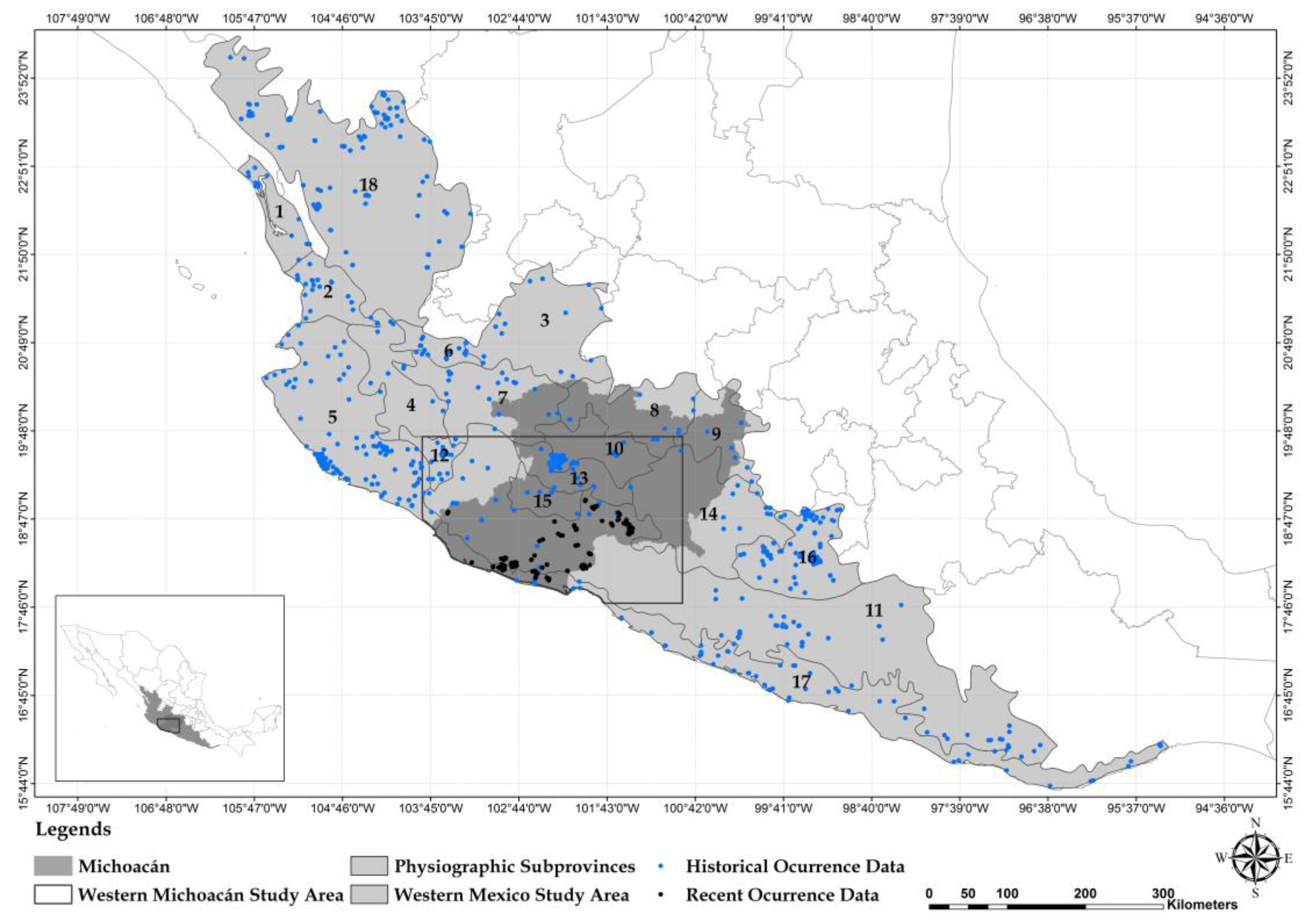
The state of Michoacán is located in the central-western part of México and includes a variety of physiographic regions [1,2] (Figure 1,

Table A1. Physiographic provinces’ general characteristics.

Physiographic Province Name	English Translation	Dominant Elevation (m)	Dominant Slope (Degrees)
Delta del Río Grande de Santiago	Río Grande de Santiago Delta	0–50	0–1
Sierras Neovolcánicas Nayaritas	Neovolcanic mountain range in Nayarit state	800–1000	4–8
Altos de Jalisco	State of Jalisco’s highlands	1800–2000	0–1
Sierra de Jalisco	State of Jalisco’s mountain range	1400–1600	8–16
Sierras de la Costa de Jalisco y Colima	Coastal mountain range in the states of Jalisco and Colima	200–400	8–16
Guadalajara	Guadalajara	1400–1600	0–1
Chapala	Chapala	1600–1800	0–1
Sierras y Bajíos Michoacanos	Mountain range and lowlands in Michoacán state	1800–2000	0–1
Mil Cumbres	Thousand summits	2200–2400	4–8
Neovolcánica Tarasca	Neovolcanic Tarasca	2200–2400	4–8
Cordillera Costera del Sur	Southern coastal mountain range	400–600	8–16
Volcanes de Colima	State of Colima’s volcanos	400–600	2–4
Escarpa Limítrofe del Sur	Southern limiting escarpment	1000–1200	4–8
Depresión del Balsas	Balsas depression	200–400	8–16
Depresión de Tepalcatepec	Tepalcatepec depression	200–400	0–1
Sierras y Valles Guerrerenses	Mountain ranges and valleys in Guerrero state	1000–1200	8–16
Costas del Sur	Southern coasts	50–100	0–20
Mesetas y Cañadas del Sur	Southern plateau and ravines	2000–2200	8–16
Nuevo Atlas Nacional de México [117]

). Michoacán’s heterogeneity in climate, physiography and lithology promotes ecological conditions that allow for the presence of a wide variety of vegetation communities [3] associated with a high fauna diversity. A high diversity of vertebrate species is found in the transition zones between physiographic regions in the state of Michoacán [4].

There are 161 mammal species reported in the state of Michoacán, which represent 32% of the species at the national level; the most represented order in the state is Chiroptera with 74 species, while Carnivora has 18 species [5].

1.2. Carnivores and Biodiversity Indicators

Carnivores play an important ecological role; these can belong to many trophic levels due to their variance in size, their separation between temporal and spatial niches, and their food habits [6,7]. Their presence and population conditions represent valuable ecological metrics because this is a group indicator of the conservation status in different ecosystems. Species of carnivores are considered to be umbrella species, since the conservation of their distribution aids in protecting many other species inhabiting the same habitats [6]. As large predators, carnivores control their prey populations, affecting the trophic web dynamics, and therefore the ecosystem’s energy flows [8].

Issues related to the global conservation of carnivores are widely documented [9,10,11,12,13,14]. Their specific food habits, their need for large areas and their low tolerance to human presence make carnivores highly vulnerable to extinction processes [15]. The strongest threats are the destruction and fragmentation of habitats and the intense hunting of them and their prey [16].

1.3. Species Distribution Models

Analyzing patterns of species distributions during the last few decades has been a research tool used in important fields such as conservation planning. Therefore, many species distribution algorithms and procedures have been developed, which aim to improve the prediction of such models [17]; such is the case for the application of geographic information systems (GIS) and the development of statistic and machine learning algorithms oriented to generate robust species distribution models [18,19,20,21,22,23,24,25,26,27,28,29,30]. Considering the wide assortment of algorithms [31], an ensemble of consensus of models has been proposed as an approach to generate more robust species distribution predictions [32].

For some authors, ecological niche modeling (ENM) is not synonymous with species distribution modeling (SDM) [33]. However, the niche concept is key to differentiating between potential (e.g., environmental envelopes) and actual distribution models (i.e., habitat suitability). Peterson and Soberón [34] recommend being careful when distinguishing between the environmental envelope models generated under the ENM approach and their existing or realized manifestations; the reconstructed distributions should necessarily consider the historical landscape transformations to obtain models of the species’ actual distributions. In this study, we followed Grinell’s [35] concept of habitat suitability to refer to species distribution models. Therefore, we differentiate between those models determined by only bioclimatic variables and topography (bioclimatic envelopes) and those determined by both land-use/land-cover suitability and bioclimatic envelopes (habitat suitability).

1.4. Conservation Areas

Historically, the establishment of natural protected areas has been based on opportunity ad-hoc criteria, which is different from systematic biodiversity knowledge [36,37]. However, currently, species distribution models are used as key input for identifying and selecting natural areas with maximum representation of species richness, meaning that computing methods have been developed for the selection of natural areas [38,39,40,41]. Such methods have focused on the following three quantitative approaches [42,43]: (a) identification of hot spots in species richness, (b) selection of areas with rare species, and (c) complementarity of natural areas.

Systematic conservation planning requires setting clear objectives from which it is possible to propose measurable and explicit conservation goals [44]. Conservation goals consist of explicitly quantifying a minimum amount of biodiversity elements, such as species distributions and vegetation types, which may be protected at local, regional, or continental scales [45].

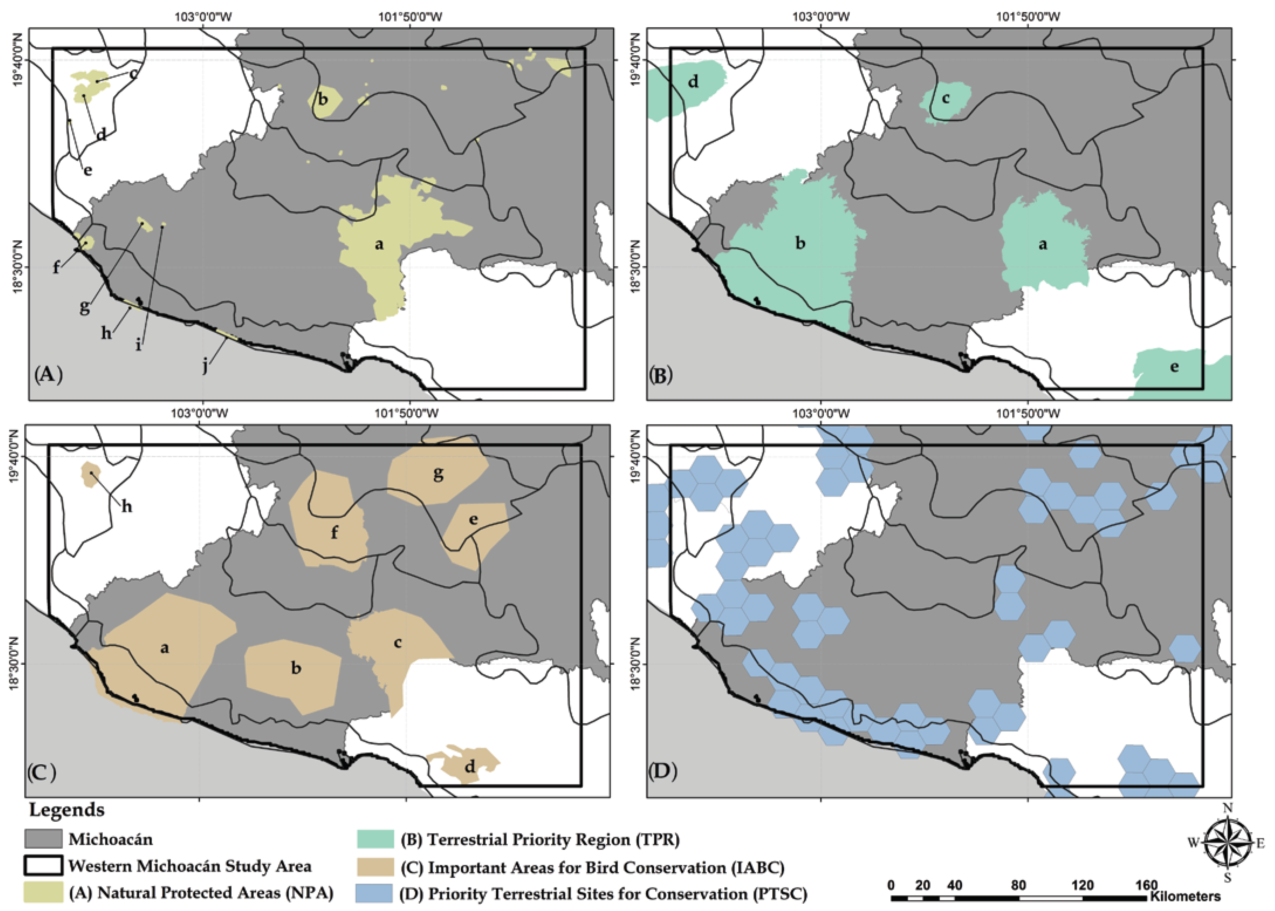
Several natural protected areas exist in western Michoacán, México, covering approximately 328,000 ha, comprised mostly of the Zincuirán-Infiernillo biosphere reserve [4,46]. Several proposals to protect this region´s natural areas also exist, including Terrestrial Priority Regions (TPR) [47], Important Areas for Bird Conservation (IABC) [48], and Priority Terrestrial Sites for Biodiversity Conservation (PTSC) [49] at the country scale (Figure 2), and Priority Areas for Conservation in Michoacán (PACM) [50] and the Conservation Areas System in Michoacán (CASM) [51] at the state scale.

1.5. Statement of the Problem

Elaborating national schemes for prioritizing mammal conservation in México has made evident the need for generating reliable species distribution models at a higher spatial resolution [52]. Most of the studies on Michoacán’s mammals have focused on estimating species richness [5,53,54,55,56,57,58]. These studies suggest that the region is crucial for the connectivity of populations, but there is no spatial analysis of how biodiversity patterns are distributed across the region.

Western Michoacán is representative of western México’s biodiversity and endemism. The Faja Transvolcánica and Sierra Madre del Sur are identified as relevant regions because of their high concentrations of endemic plants and animals [59]. There are various aspects that explain this region’s research and biodiversity conservation challenges. For example, the region is representative of the entire biodiversity in western México’s slope, including various species of carnivores. There is a lack of information about the regional patterns of biodiversity and the biosphere reserve Zicuirán-Infiernillo (ZIBR) is the only large natural protected area, as the remaining areas are not significant in terms of size and care. There are several proposed areas defined as priorities for conservation, with some of them comprising very large areas. Finally, the region has experienced significant changes in land-use/land-cover, reducing and altering natural habitats for wildlife, including carnivore species.

This study aims to determine the level of spatial correspondence between natural protected areas (NPA) and the existing proposed areas for conservation, with actual hot spot areas identified based on the distribution of carnivore species. One research question relates to the ZIBR’s role in protecting areas with high carnivore richness and the specific priority sites within the large regions proposed for conservation.

This study considers a group of carnivores as a biodiversity indicator, whose spatial patterns of richness and rareness would suggest the location of areas that should be considered as priority for conservation. This analysis or selection of areas also includes vulnerability conditions resulting from deforestation and fragmentation processes. We propose models of suitable habitats of carnivore species in western Michoacán, México, generated from bioclimatic envelopes and habitat/species associations, corresponding to western México. We also propose to obtain estimates of vulnerability in areas where carnivore species are distributed, due to deforestation and fragmentation processes (i.e., land-use/land-cover changes), and identify important areas for conservation, by applying systematic conservation planning tools (e.g., prioritization and complementarity), based on the distribution of suitable habitats of carnivore species and the potential transformation in the land cover.

2. Materials and Methods

2.1. Carnivore Species Occurrence Data

Occurrence data of carnivore species in western Michoacán were obtained from field work carried out during the years 2010–2014, which was part of a project named “Jaguar Conservation” (unpublished study). These data were collected by a photo-trap system. We installed between 15 and 30 photo-trap stations per sampling site. The stations were uniformly distributed according to a grid and the landscape characteristics, separated 1.5–2.5 km from each other. The digital cameras used were the Cuddeback brand (PO Box 10447, Green Bay, WI 54307) and the capture and ambush model. The cameras were active for 24 hrs for 1.5–2.5 months. The stations were situated on trails used mainly by wild felines and waterholes. Sampling was mainly carried out during the dry season, between February and July, without using lures. The location of stations is shown in Figure 1.

On the other hand, historical occurrence data of carnivore species in western México were acquired from accessing the following different databases: Global Biodiversity Information Facility (GBIF), Mammal Networked Information System (MaNIS), Unidad de Informática para la Biodiversidad UNAM (UNIBIO), and Comisión Nacional para el Conocimiento y Uso de la Biodiversidad (CONABIO). These databases are public and they were cleaned and integrated into a single database, avoiding duplicates and records without complete taxonomic and georeferenced data.

A preliminary species list of carnivores in Michoacán [5] and the recorded species by Nuñez (unpublished data) were used to verify their taxonomic status following the work of Ramirez-Pulido et al. [60,61] and supported by the work of Ceballos et al. [62,63], and CONABIO. Eleven species were finally included in this study, as shown in

Table 1. Carnivore species, conservation status and record number by species in two databases, wMex (western México) and wMich (western Michoacán). Taxonomy according to Ramírez-Pulido et al. [60].

Family	Species	Conservation Status			Number of Records
		SEMARNAT a	CITES b	IUCN c	wMex	wMich
CANIDAE	Canis latrans (Say, 1823)				216	25
	Urocyon cinereoargenteus (Schreber, 1775)				366	20
FELIDAE	Herpailurus yagouaroundi (Lacépède, 1809)	A	I	EN	91	6
	Leopardus pardalis (Linnaeus, 1758)	P	I	EN	127	43
	Leopartus wiedii (Schinz, 1821)	P	I	NT	77	11
	Puma concolor (Linnaeus, 1771)				97	33
	Panthera onca (Linnaeus, 1758)	P		NT	84	18
MEPHITIDAE	Conepatus leuconotus (Lichtenstein, 1832)				231	6
PROCYONIDAE	Bassariscus astutus (Lichtenstein, 1830)				239	6
	Nasua narica (Linnaeus, 1766)		III		376	81
	Procyon lotor (Linnaeus, 1758)				242	14
TOTAL RECORDS					2146	263

^a SEMARNAT: Mexican federal natural resources protection agency. ^b CITES: Convention on International Trade in Endangered Species of Wild Fauna and Flora. ^c IUCN: International Union for Conservation of Nature. ^c IUCN: NT = close to threatened; EN = endangered. ^a NOM-059-SEMARNAT-2010: P = endangered; A = threatened. ^c I (Appendix A) = species that are more endangered. ^c III (Appendix A) = species included at the request of a party that already regulates trade in the species and that needs the cooperation of other countries to prevent unsustainable or illegal exploitation.

.

Table A2. Characteristics of study species.

Family	Species	Common Name	Description
CANIDAE	Canis latrans Say, 1823	Coyote	Medium-size canid. Social animals with twilight activity. They have a total length of between 1075 and 1150 mm and a weight between 8 and 16 kg. Generalist food habits with seasonal variations, including lagomorphs, rodents, ungulates, fruits, insects, reptiles, and birds. Their home range size is inverse to population density. For resident individuals, it is higher in adults than juveniles (5 vs. 2.4 km2); and it is even higher for transient individuals. They live in every vegetation type in México, particularly in plains with desert scrub and grassland.
	Urocyon cinereoargenteus (Schreber, 1775)	Gray fox	Medium-size canid with a 500–600 mm total length and 3–5 kg weight. Opportunistic feeding habits, consuming rodents, lagomorphs, fruit, and insects. Home range varies from 1 to 8 km2, depending on the season, population density and habitat quality. They live mainly in forests and shrubland, but can also live in every vegetation type, from sea level to 3500 masl.
FELIDAE	Herpailurus yagouaroundi (Lacépède, 1809)	Jaguarundi	As a felid, it is a small animal (888–1372 mm total length and 3.5–9 kg weight). It can be found in tropical evergreen and dry forests, but can also live in mangroves, cloud forests, desert scrubs, and occasionally in temperate forests, from sea level to 2000 masl. It is well adapted to arboreal environments and its food habits consist of a wide range of prey, including invertebrates, reptiles, birds, and small mammals. Its activity area is 88.8- 99.9 km2 for males and 20.1 km2 for females.
	Leopardus pardalis (Linnaeus, 1758)	Ocelot	This is a medium-size felid (920–1367 mm total length and 6–15 kg weight). Lives mainly in tropical evergreen forests, tropical forests and mangroves, but also in cloud forests and desert scrubs occasionally. It can be found from sea level to 2000 masl. Prefers dense land-cover habitats and feeds on small and medium-size rodents, but also on invertebrates, reptiles, birds and other mammals, including the temazate deer. Its activity area varies from 3.5 to 17.7 km2 for males and 0.7–14.6 km2 for females.
	Leopartus wiedii (Schinz, 1821)	Margay	Small-size felid with 805–1300 mm total length and 3–5 kg weight. It is the most arboreal of México’s felids, because it sleeps, rests and hunts in trees. Lives in tropical evergreen and tropical dry forests, mangroves, and cloud forests, from sea level to 3000 masl. It feeds on invertebrates, birds, and small mammals, mainly rodents.
	Puma concolor (Linnaeus, 1771)	Mountain lion/cougar	This is a large-size felid with a 1100–2200 mm total length and 38–110 kg weight. They have solitary habits. They can be found in every vegetation formation of México, being the most abundant in temperate forests, from sea level to 3500 masl. This species is more tolerant to human presence than the jaguar and feeds on large rodents, armadillos, deer, peccaries and even rats and rabbits. Its activity area varies from 66 to 685 km2 for females and 152–826 km2 for males.
	Panthera onca (Linnaeus, 1758)	Jaguar	This is the largest felid in América, with a 1574 a 2419 mm total length and 36–158 kg weight. Lives mainly in tropical evergreen and tropical dry forests and mangroves, but also in cloud forests, thorny forests, desert scrubs, and temperate forests, from sea level to 2000 masl. It is considered as an opportunistic carnivore because its diet is broad and depends on prey availability and density. More than 85 species have been reported as part of its diet, including invertebrates, fish, reptiles, birds, and mammals. Its activity areas are 10–38 km2 for females and 28–90 km2 for males.
MEPHITIDAE	Conepatus leuconotus (Lichtenstein, 1832)	White-backed skunk	These are the largest skunks with a size similar to a domestic cat. Its total length is 410–633 mm with a 900–4500 g. Lives in a variety of environments, from temperate to desert and tropical environments, including thorny forests, tropical dry forests, scrubland, grassland, temperate forests, and crop land, from sea level to 2500 masl. It feeds on invertebrates such as insects (mainly beetles), worms, fruits, small vertebrates, and occasionally carrion. They are solitary animals. In México, four individuals per square kilometer densities have been reported.
PROCYONIDAE	Bassariscus astutus (Lichtenstein, 1830)	Ringtail	This is a medium-size carnivore with a 616–811 mm total length and 870–1100 g weight. Lives in desert scrubs, temperate forests, tropical semi-desert, scrubland, and even urban parks, from sea level to 2880 masl. It is an omnivore and feeds mainly on small mammals, insects, fruits, birds, reptiles and occasionally nectar. They are solitary animals with nocturnal habits. Its activity area is variable and depends on habitat type, season, and sex.
	Nasua narica (Linnaeus, 1766)	White-nosed coati	Procyonids with a size similar to a medium size dog (850–1.340 mm total length and 4–6 kg weight). It is a highly social species, gathering in groups of up to 20 individuals, made up of almost exclusively adult females and juveniles. It is an omnivore collector animal that feeds mainly on fruits and invertebrates such as insects, myriapods, arachnids, crustaceans, and annelids. To a lesser extent, they hunt terrestrial vertebrates, such as rodents, amphibians and reptiles. They can be found mainly in tropical evergreen and tropical dry forests, but they are also common in temperate forests and desert scrubs, from sea level to 2900 masl.
	Procyon lotor (Linnaeus, 1758)	Raccoon	Medium-size procyonid with a 603–950 mm total length and 3–9 kg weight. It has twilight and nocturnal habits. They have adapted to a wide variety of habitat types with permanent water bodies. They are more abundant in tropical evergreen and tropical dry forests, mangroves, and areas with aquatic and semi-aquatic vegetation associated with marshes, swamps, and wetlands, from the sea level to almost 3000 masl. It is an omnivore and feeds on a wide variety of plant and animal foods. It is considered as a solitary species and its activity area widely varies from 0.2 to 4946 ha, although a typical annual average is 65 ha for males and 39 ha for females.

provides general information about the species’ biological and ecological characteristics.

This study used a total of 263 occurrence records that belonged to 11 carnivore species found in western Michoacán during the years 2010–2014. Nasua narica was the species with the highest number of records (81), while Bassariscus astutus, Conepatus leuconotus and Herpailurus yagouaroundi had the lowest with six records. On the other hand, a total of 2146 historic occurrence records, for the same 11 carnivore species but across western México, were integrated from querying public databases. The highest number of records belonged to Nasua narica (376), while the lowest was Leopardus wiedii with 77 records (Table 1).

2.2. Species Distribution Modeling

Species distribution models were generated by applying a consensus approach [32]. The software MODECO [64] was used to run the following different prediction algorithms: support vector machines (SVM), generalized linear models (GLM) and artificial neural networks (ANN). MaxEnt (maximum entropy) was also applied, but it was run independently because its software provides a more complete analysis.

2.3. Prediction Variables

The variables for predicting the species bioclimatic envelopes in western México included topography (elevation and aspect) and 19 bioclimatic variables (see

Table 2. Variables used in the elaboration of bioclimatic envelope models for carnivore species in western México. Selected variables per species represented ≥95% in prediction importance. A complete set of variables was used to select the important prediction variables for each species.

Species (Order Carnivora)	Prediction Variables
	Bioclimatic Variables																			Topo
	b1	b2	b3	b4	b5	b6	b7	b8	b9	b10	b11	b12	b13	b14	b15	b16	b17	b18	b19	asp	ele
Canis latrans (Say, 1823)		X		X	X	X						X	X	X				X	X	X	X
Urocyon cinereoargenteus (Schreber, 1775)				X			X	X	X			X		X		X	X		X		X
Herpailurus yagouaroundi (Lacépède, 1809)		X				X	X							X		X	X		X	X	X
Leopardus pardalis (Linnaeus, 1758)		X	X	X		X	X				X	X									X
Leopartus wiedii (Schinz, 1821)		X	X	X			X						X				X
Puma concolor (Linnaeus, 1771)			X	X								X					X	X	X	X
Panthera onca (Linnaeus, 1758)			X	X			X										X	X		X	X
Conepatus leuconotus (Lichtenstein, 1832)		X		X		X	X	X	X					X			X	X
Bassariscus astutus (Lichtenstein, 1830)		X	X		X				X			X	X	X	X			X			X
Nasua narica (Linnaeus, 1766)	X	X				X	X	X	X		X	X		X			X	X			X
Procyon lotor (Linnaeus, 1758)		X						X	X			X		X					X	X

Topo = topographic, asp = aspect; ele = elevation. Bioclimatic variables: b1 = annual mean temperature; b2 = mean diurnal range (mean of monthly values (max temp–min temp); b3 = isothermality (b2/b7) (×100); b4 = temperature seasonality (standard deviation ×100); b5 = max temperature of warmest month; b6 = min temperature of coldest month; b7 = temperature annual range (b5-b6); 8 = mean temperature of wettest quarter; b9 = mean temperature of driest quarter; b10 = mean temperature of warmest quarter; b11 = mean temperature of coldest quarter; b12 = annual precipitation; b13 = precipitation of wettest month; b14 = precipitation of driest month; b15 = precipitation seasonality (coefficient of variation); b16 = precipitation of wettest quarter; b17 = precipitation of driest quarter; b18 = precipitation of warmest quarter; b19 = precipitation of coldest quarter.

for a description) from the WorldClim project [65] (https://www.worldclim.org/ (accessed on 19 July 2020). This data set (21 variables) was used to generate preliminary bioclimatic envelope models, allowing the selection of more significant prediction variables. The selected variables differed in number and composition for each species, and they accounted for ≥95% of the total percentage. All of these environmental variables have a spatial resolution of about 1 × 1 km² in geographic coordinates.

2.4. Bioclimatic Envelope Models

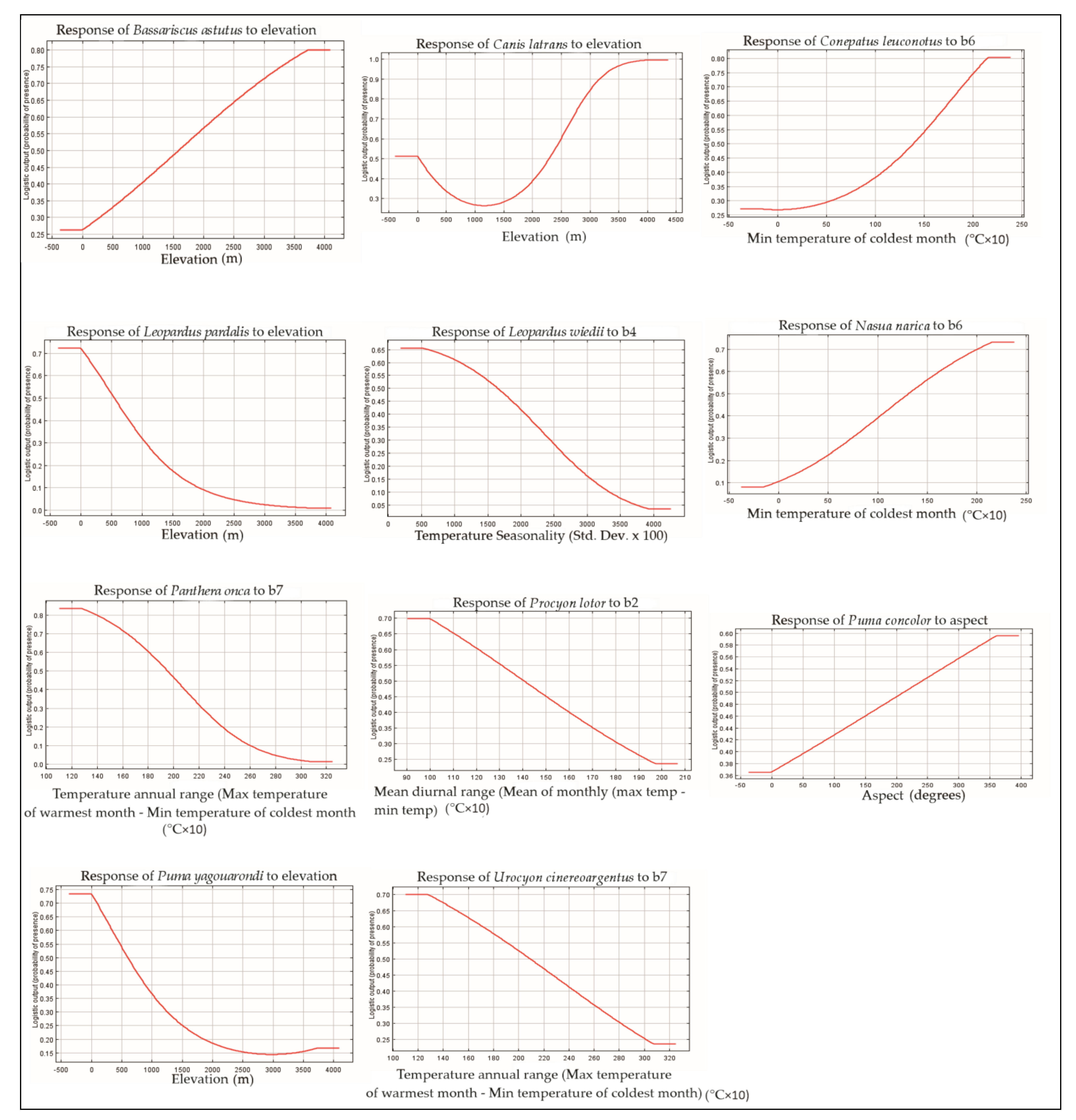
Maxent [66] was the algorithm applied to generate bioclimatic envelope models for selecting important prediction variables, using the complete set of climate (n = 19) and topography (n = 2) variables. We used MaxEnt’s default settings with linear and quadratic feature types and 30% of the samples for accuracy assessment. The selected prediction variables for each species are shown in Table 2 and the response curves of the most important prediction variables appear in Figure A1. These selected variables were then used to run four different prediction algorithms per species, whose general settings are as follows: MaxEnt as previously described; support vector machines (C-SVC as SVM types and radial basis function kernel); generalized linear models (logit link function); artificial neural networks (prob-ANN trained based on backpropagation, 0.3 momentum and 0.1 learning rate). The algorithms applied were chosen because these were considered to be promising prediction tools [67,68] and are included in a group of algorithms in ModEco that run with presence data vs. backgrounds.

Four models for each species, for a total of forty-four bioclimatic envelope models, were constructed by applying the algorithms MaxEnt, support vector machine, generalized linear model and artificial neural networks. Afterwards, a consensus approach [32] was applied, so that the median was the representative statistic for combining four prediction models for each species.

2.5. Habitat Suitability Models

Considering that occurrence data for the carnivore species distributed in western Michoacán were recently collected (2010–2014), generalized linear models (GLM) were run to estimate habitat associations, a type of analysis that required pseudo absence data. These data for each carnivore species were generated from those bioclimatic envelope models obtained for western México. By applying this approach, it was expected to reduce the risk of generating pseudo absences in places that were potentially suitable for the species, in contrast with the random approach that is often suggested [69,70]. The use of preliminary habitat suitability maps as a spatial guide for generating pseudo absences is an efficient means to reduce the possibility for obtaining false negatives [70,71].

GLMs are an extension of linear models and allow us to manage data sets that lack normal error distributions and constant variances. Binary response variables, such as presence/absence data, show these characteristics, meaning that the association between carnivore species occurrence and habitat types in western Michoacán was described by the GLM run in the software R (R Core Team, 2013). The independent variables consisted of land-use/land-cover data obtained for the years 2013–2014 (INEGI-Serie V) [72,73] and the topographic position index [74]. INEGI’s data consisted of vector coverage and a 1:250,000 scale, which was rasterized to 250 × 250 m² resolution. Therefore, the independent variables consisted of land-cover categorical variables; temperate forest, tropical semi-evergreen forest, tropical dry forest, introduced grassland, cropland, bare soils, water bodies and urban settlements. The only independent numeric variable was the topographic position index (TPI), which consists of differentiating landforms, based on elevation gradients; flat or near continuous slopes are shown by values near to zero, ridge or hill areas by large positive values, and the bottom of valleys or gullies by large negative values [74]. The significance of variables in the GLM was obtained by applying the Akaike information criterion.

Habitat suitability models for western Michoacán were obtained by adjusting the bioclimatic envelope models for western México by using the species/habitat association (probability) models obtained from the GLM analysis. A weighted sum of both types of models—the bioclimatic envelope and habitat associations—was conducted, assigning a weight of 2 to the former and 1 to the latter, and then the models were re-scaled to a 0–1 range of values. The results yielded continuous models that represented the estimates of habitat suitability for 11 carnivore species distributed in western Michoacán, determined not only by the climate and topography, but also by the land-cover conditions at the time when the species occurrence data were gathered in the field. We resampled the higher resolution models (i.e., species/habitat-type associations, 250 × 250 m) to the lower resolution models (i.e., bioclimatic envelope models, 1 × 1 km).

2.6. Model Validation

The evaluation of the models consisted of applying the partial ROC test (receiver operating characteristic) [75], which provides the partial and ratio values of the area under the curve (AUC), among other statistics. This approach has been proposed because it removes the emphasis on absence data, emphasizes the role of omission error when evaluating niche model predictivity and analyzes limited sectors of the ROC space that are not directly relevant [75]. The application of partial ROC was carried out by employing the NicheToolBox [76] (http://shiny.conabio.gob.mx:3838/nichetoolb2/ (accessed on 3 March 2021), using 30% of the training records with 500 iterations and calculating the AUC average [76].

2.7. Land-Use/Land-Cover Change

A land-use/land-cover modeling exercise was conducted to obtain the deforestation vulnerability estimates (i.e., deforestation likelihood) to be incorporated into the identification of priority areas for the conservation of carnivore species in western Michoacán. Vector coverages on a 1:250,000 scale, generated by the Mexican government (Instituto Nacional de Estadística y Geografía, INEGI) and known as Serie II [77] and Serie V [78], were used as two different dates to determine the changes in the region’s land use/land cover. Indeed, Serie II was created using Landsat TM images gathered in 1993, while Serie V was elaborated based on SPOT images gathered in 2012-13.

The Land Change Modeller module in the IDRISI Selva software was used to generate probability transition models related to the following three main submodels: deforestation (change from conserved temperate and tropical forests to cropland and introduced grassland); regeneration (change from cropland and introduced grassland to conserved and secondary temperate and tropical forests); disturbance (change from conserved temperate and tropical forests to secondary forests). This study focused on the transition probability estimates that corresponded to the deforestation submodel, because these estimates of deforestation vulnerability were included as key variables in the identification of priority areas for the conservation of 11 carnivore species in western Michoacán. Given the nature of the transition probability output, it was necessary to calculate the inverse and to rescale values from a 0–<1.0 range to 0–1.0, so that the model represented the probability of persistence of the different land-cover/land-use types. For instance, high values represented areas with low probability of change (high persistence) and low values represented high deforestation or low persistence probabilities.

2.8. Identification of Priority Areas for Conservation

Individual habitat suitability models by species were summated (1 model per species, 11 models in total) to identify areas with a high concentration of suitable species habitats or richness estimates. Continuous models were converted to binary models (i.e., presence/absence) based on the application of a prediction threshold. In this case, such a threshold consisted of the sensibility/specificity maximization criteria [79] (see

Table A3. Prediction threshold for transforming continuous habitat suitability models to binary models.

Species	Sensibility/Specificity Maximization Threshold
Bassariscus astutus	0.31
Canis latrans	0.24
Conepatus leuconotus	0.26
Leopartus pardalis	0.34
Leopartus wiedii	0.23
Nasua narica	0.44
Puma concolor	0.64
Procyon lotor	0.28
Panthera onca	0.32
Herpailurus yagouaroundi	0.33
Urocyon cinereoargenteus	0.39

).

The software Zonation v1.0 [80] was used to prioritize the analysis of conservation areas. Zonation is based on the complementarity of areas and serves as a balance to rank conservation priorities across the landscape through the iterative elimination of cells or planning units to direct at a minimum aggregated loss of conservation values. The cell elimination order depends on an elimination rule, which can be selected according to conservation objectives [80,81,82].

The suitable habitat models (continuous) for each species and the inverse deforestation model were used as inputs, while the additive benefit function (ABF) and the core area zonification (CAZ) were applied as removal rules. In general terms, the ABF rule exclusively prioritizes exclusively high richness areas, whereas the CAZ rule determines important high richness areas, while at the same time identifies areas with unique biodiversity elements (e.g., rareness areas).

Different weights were assigned to each species, depending on their conservation status (see

Table 3. Weights assigned to each species in the prioritization of conservation areas. A higher weight represents the highest level of concern considered by the prioritization algorithm (zonation).

SPECIES	Conservation Status (NOM059)	Weight
Canis latrans (Say, 1823	-	1
Urocyon cinereoargenteus (Schreber, 1775)	-	1
Herpailurus yagouaroundi (Lacépède, 1809)	T	2
Leopardus pardalis (Linnaeus, 1758)	EN	3
Leopartus wiedii (Schinz, 1821)	EN	3
Puma concolor (Linnaeus, 1771)	-	1
Panthera onca (Linnaeus, 1758)	EN	3
Conepatus leuconotus (Lichtenstein, 1832)	-	1
Bassariscus astutus (Lichtenstein, 1830)	-	1
Nasua narica (Linnaeus, 1766)	-	1
Procyon lotor (Linnaeus, 1758)	-	1

NOM059 = legal conservation status by the Mexican government [83]. EN = endangered. T = threatened.

) and different modeling parameters were used. Smoothing and boundary length penalty (BLP) are two aggregation methods that generate solutions more compactly. The former conserves well-connected areas and the latter is the most frequently used method. Additionally, BLP does not consider situations such as species fragmentation, but rather impacts the boundary length to produce more compact conservation areas.

Different conservation priorities are classified in the resulting conservation models, allowing for the specification of different thresholds in the percentage of landscape. For instance, 15% of the landscape is sometimes chosen as a threshold to describe the conservation areas identified.

2.9. Comparing Identified and Already Proposed Priority Areas

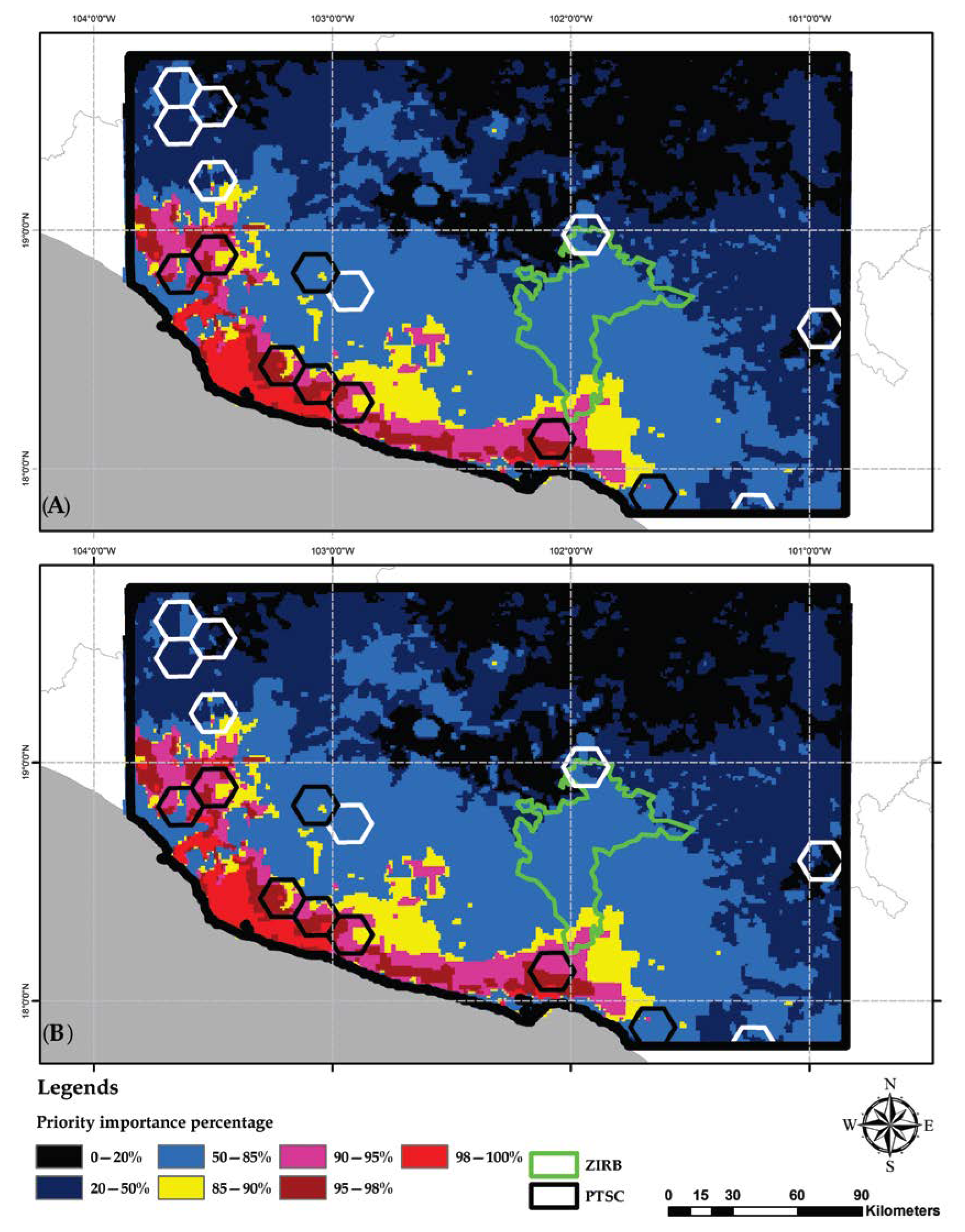
The conservation areas identified in this study were compared (overlap) with other existing areas that have been proposed for conservation. Particular attention is paid to a recent version of the priority terrestrial conservation areas (RTP) proposed by CONABIO [49] (Priority Terrestrial Sites for Biodiversity Conservation (PTSC); see Figure 2), which consist of 256 km² hexagons distributed across the country and with a ranked priority level (medium, high and very high).

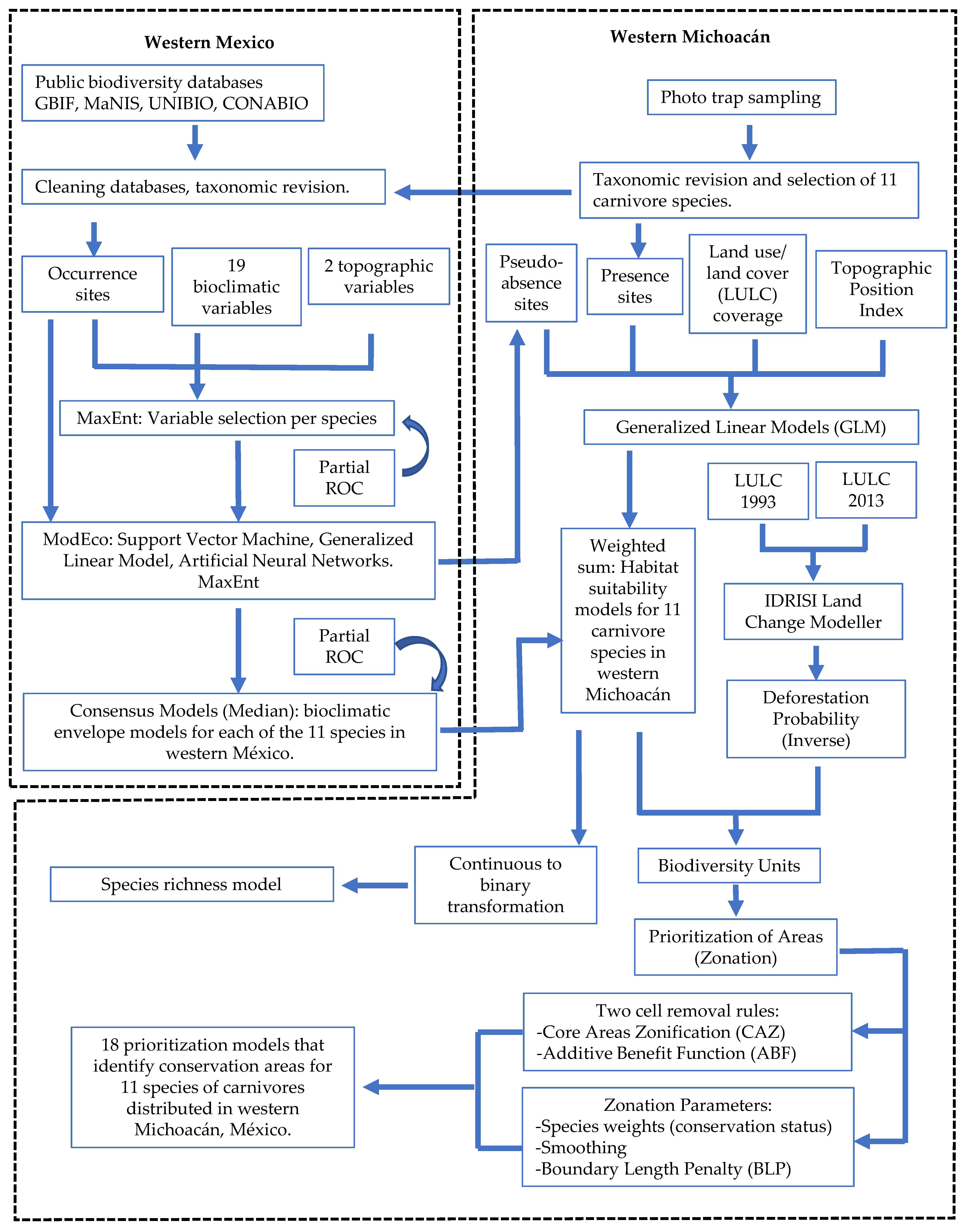
A flow diagram, as shown in Figure 3, helps us to explain and clarify the different steps taken in the applied methods.

3. Results

3.1. Variable Importance

The most important prediction variables varied among species (Table 2); 13 variables predicted 5–8 species and 8 variables predicted <5 species (see Table 2). The b10 variable (mean temperature of warmest quarter) was not important for any species, while b2 (mean diurnal range (Mean of monthly values (max temp–min temp)) was important for eight species.

3.2. Associations Species/Habitat Types

Table 4. Parameters obtained by generalized linear models (GLM) for estimating the habitat type/species associations.

SPECIES (ORDER CARNIVORA)	Dispersion Parameters
	Presence/Absence Records	Significant Variables	Deviance Null	Deviance Residual	Deviance (D2)	Estimate	AIC	Z Value	p Value
Canis latrans	25/25	TPI	205.1	143.2	30.1%	0.002014	171.2	1.841	0.0656
Urocyon cinereoargenteus	20/20	TPI/ Oak Forest	213.4	164.9	22.7%	0.00322/ −2.747	190.9	3.142	0.00168/ 0.092
Herpailurus yagouaroundi	6/6	(-)	30.4	22.7	25.5%	-	38.7	(-)	(-)
Leopardus pardalis	43/43	TPI	155.2	105.7	31.8%	0.003406	137.7	2.365	0.018
Leopartus wiedii	11/11	TPI	72.0	34.3	52.3%	0.004993	60.3	1.942	0.0522
Puma concolor	33/33	TPI	130.3	44.8	65.5%	0.008745	78.8	3.231	0.00123
Panthera onca	18/18	TPI	55.4	20.6	62.6%	0.00834	42.6	1.719	0.0855
Conepatus leuconotus	6/6	(-)	63.7	36.7	42.4%	-	60.7	(-)	(-)
Bassariscus astutus	6/6	(-)	77.6	39.9	48.5%	-	65.9	(-)	(-)
Nasua narica	81/81	TPI	291.1	179.2	38.4%	0.003061	215.2	2.942	0.00327
Procyon lotor	14/14	(-)	88.7	57.4	35.2%	-	85.4	(-)	(-)

shows a summary of the estimated association probability between habitat types and each species’ presence (GLM analysis) in western Michoacán. All models had a partial ratio AUC value above 1.2, which indicates good-fitting models.

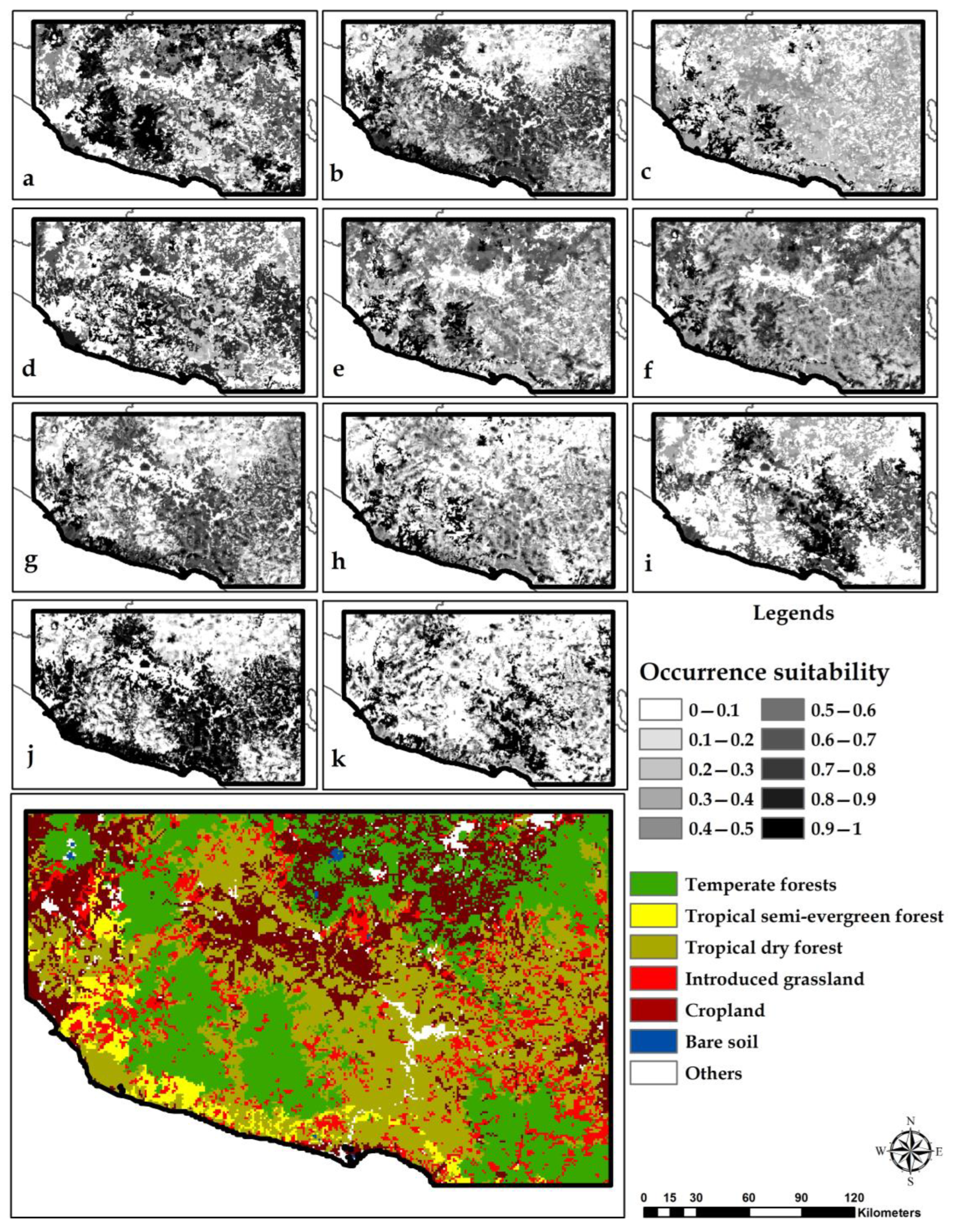
The results indicate that the lowest probability areas for all the species correspond to bare soil and cropland areas. Some species also showed low occurrence probabilities in other land-cover types; for instance, Urocyon cinereoargenteus, Herpailurus yagouaroundi and Leopardus pardalis in temperate forests, and Conepatus leuconotus and Bassariscus astutus in tropical semi-evergreen forests (Figure A2).

The high occurrence probability areas for Urocyon cinereoargenteus, Leopardus pardalis and Nasua narica consisted of almost exclusively tropical semi-evergreen forests for the species Canis latrans, Leopardus wiedii and Procyon lotor. The highest presence probability areas were areas with tropical semi-evergreen forests and temperate forests, whereas Panthera onca was highly associated with tropical semi-evergreen forests and tropical dry forests. Temperate forests are areas where Conepatus leuconotus and Bassariscus astutus had the highest occurrence probability, while tropical dry forests were the land-cover types with the highest probability for Herpailurus yagouaroundi and Puma concolor (see Figure 4).

Regarding the GLM statistical model, the topographic position index (TPI) was the independent variable with significative influence when predicting the presence of the following seven species: Canis latrans (p = 0.065), Leopardus pardalis (p = 0.018), Leopardus wiedii (p = 0.052), Puma concolor (p = 0.0012), Panthera onca (p = 0.085), Nasua narica (p = 0.0032) and Urocyon cinereoargenteus (p = 0.0016). This last species also showed a low p-value (0.092) for the variable “oak forest”, but with a negative relationship (Estimate = −2.432), which indicates that the occurrence probability increases as the distance of the species’ location increases.

3.3. Habitat Suitability Models

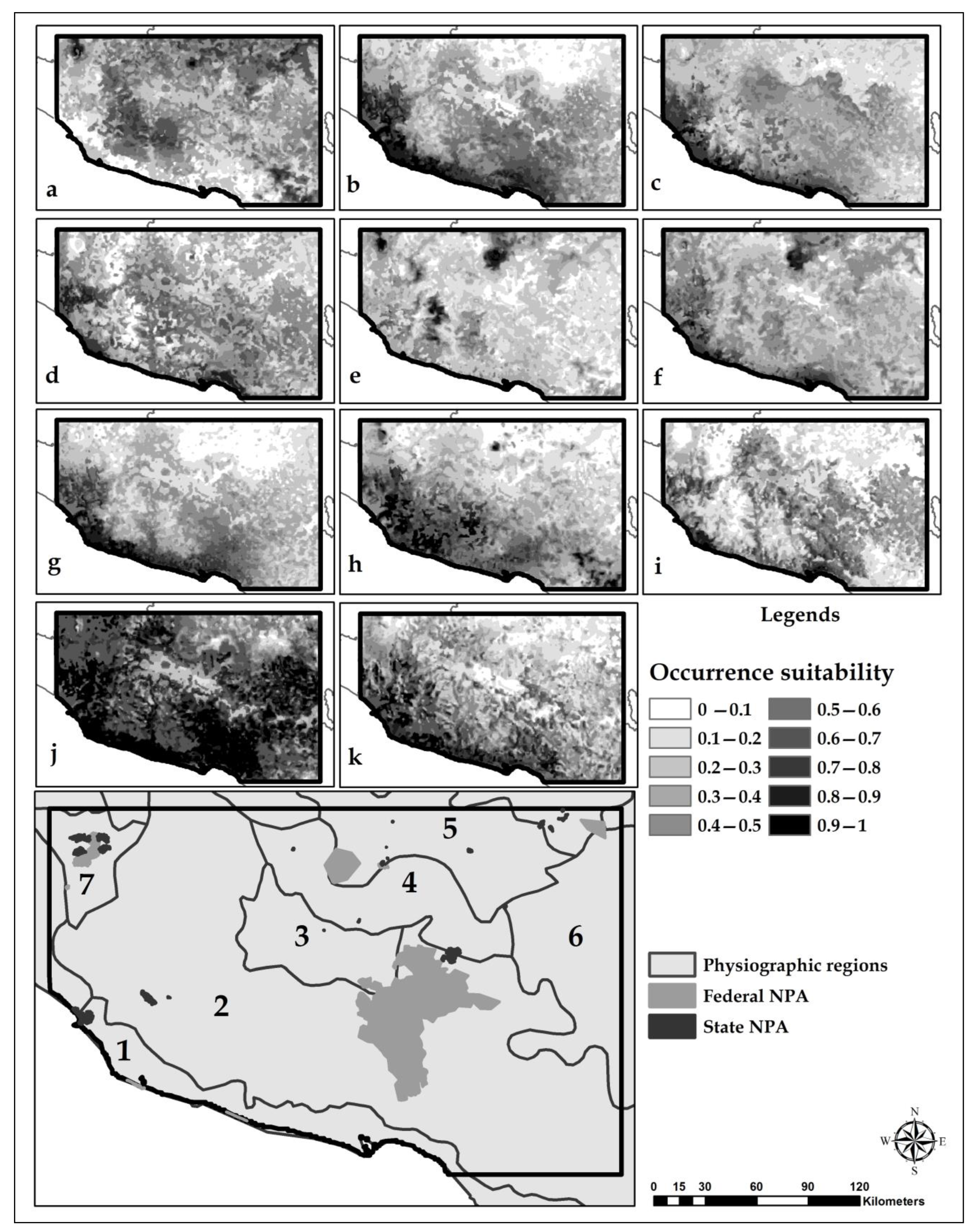
The habitat suitability models for each species were obtained by the weighted sum of the bioclimatic envelope models for western México and habitat/species associations models for western Michoacán. Seven species (Urocyon cinereoargenteus, Herpailurus yagouaroundi, Leopardus pardalis, Panthera onca, Conepatus leuconotus, Nasua narica and Procyon lotor) showed suitable habitats almost exclusively in the Michoacán coast region, corresponding to the Costas del Sur physiographic province, including counties (“municipios”) such as Aquila, Coahuayana, Chinicuila, Lázaro Cárdenas, Coalcomán and Arteaga, zones covered by tropical dry forest and tropical semi-evergreen forest (Figure A3).

The suitable habitats of these seven species are partially included in small natural protected areas (NPA), such as “Lagunas Costeras y Serranias Aledañas a la Costa Norte de Michoacán”, “Playa Maruata y Colola” and “Playa Mexiquillo” sanctuaries; the Terrestrial Priority Region (TPR) “Sierra de Coalcomán”; the Important Area for Bird Conservation (IABC) “Coalcomán-Pomaro”; polygon 6 in the Priority Areas for Conservation in Michoacán (PACM); and areas 01 and 02 in the Conservation Areas System in Michoacán (CASM). Nevertheless, recent records exist for most species within the “Zicuirán Infiernillo” biosphere reserve (ZIBR); only Panthera onca y Puma concolor showed high occurrence probability within this area (Figure A3).

The other four species (Canis latrans, Leopardus wiedii, Puma concolor and Bassariscus astutus) showed suitable habitats, expanding from the coastal region towards inland Michoacán, including the Costas del Sur and Cordillera Costera del Sur physiographic provinces (Figure A3). Temperate forest is the main vegetation type in this latter province.

Bassariscus astutus is the species that showed the most restricted suitable habitats in western Michoacán; small areas with high occurrence probability are found in the Cordillera Costera del Sur province (Figure A3), within the Coalcomán and Aguililla counties. On the other hand, Puma concolor was the species with the most widespread suitable habitats. It is important to mention that the Depresión del Tepalcatepec province did not include species with high occurrence probability because it is largely covered by cropland.

3.4. Land-Use/Land-Cover Change

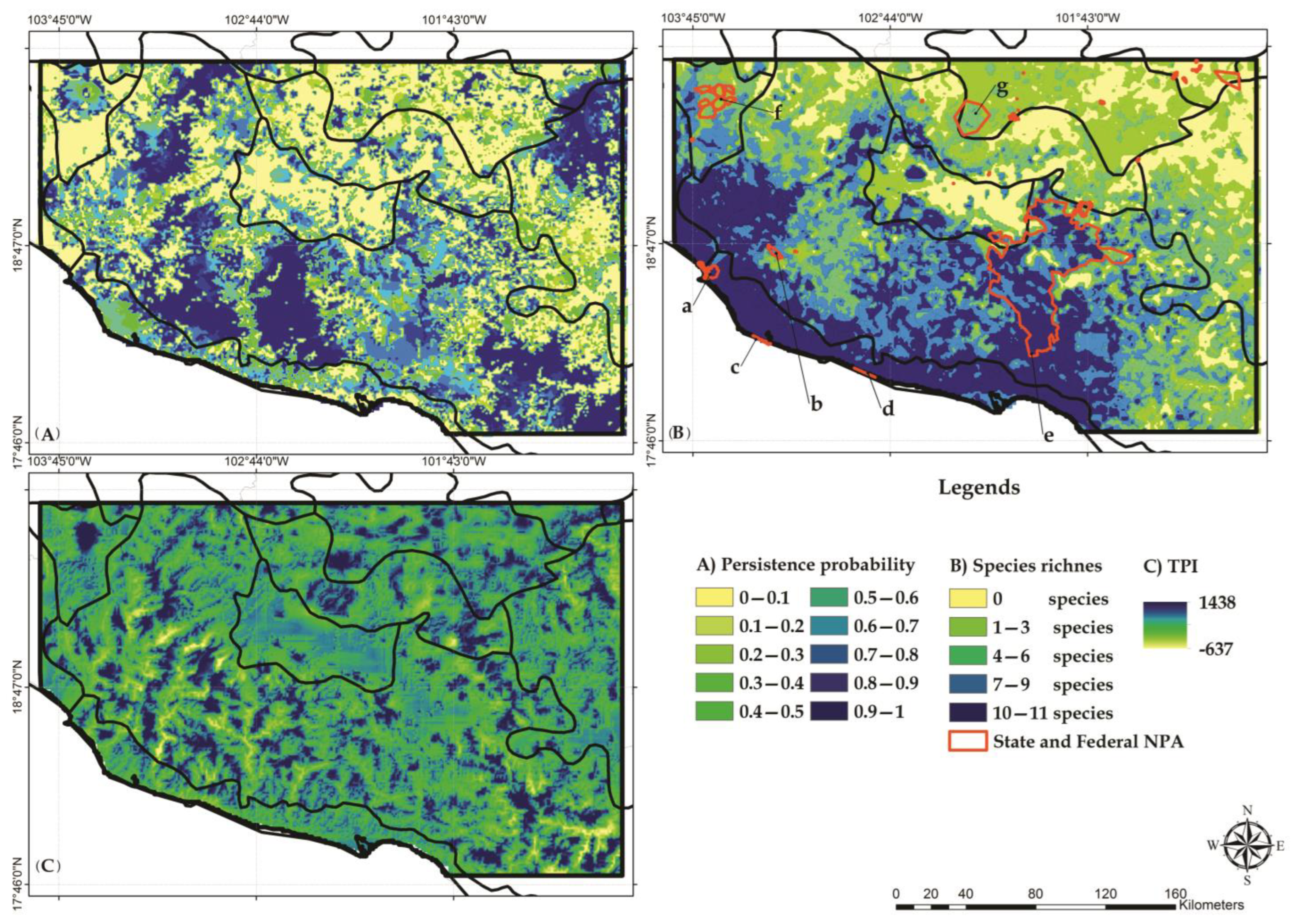
The highest values in the inverted deforestation model correspond to temperate forest areas, while the lower values are associated with tropical forest areas (Figure 4A). Apparently, temperate forests in western Michoacán have been transformed at lower rates than tropical formations within the time-period 1993–2014. Inference can be made that tropical forests have higher vulnerability to the deforestation processes that occur in western Michoacán.

3.5. Identification of Conservation Priority Areas

A species richness model was created by adding together the individual binary habitat suitability models for western Michoacán. This richness model shows that more species (e.g., 10–11 species) co-occur in the Costas del Sur physiographic province, involving the counties of Coahuayana, Aquila and Lázaro Cárdenas. However, there are small high richness areas scattered across the region. The Cordillera Costera del Sur province included 7–9 richness values, while the Depresión de Tepalcatepec province included mainly low richness values (1–3 species; Figure 4B).

One small NPA (“Lagunas Costeras y Serranías Aledañas de la Costa Norte de Michoacán”) and two sanctuaries demonstrated spatial correspondence with the highest richness areas within the Costas del Sur province. The ZIBR, located in the Cordillera Costera del Sur province, also included high species richness areas (7–9 species).

Currently, the proposed priority areas and regions for conservation have not been actualized due to issues of size (exceptionally large or exceedingly small). Thus, important portions of the TPR, including “Sierra de Coalcomán” and the IABC “Coalcomán-Pomaro”, as well as polygon 6 in PACM, areas 01 y 02 in CASM, the sanctuaries “Playa de Maruata y Colola” y “Playa Mexiquillo”, and a small area of NPA “Lagunas Costeras y Serranías Aledañas de la Costa Norte de Michoacán”, all show spatial correspondence with the high-priority conservation areas identified by the 18 priority models. The southern portion of ZIBR also included high-priority areas. To a lesser extent, other areas also contain identified priority areas, such as the NPA “Pico de Tancíntaro”, “El Jabalí”, “Volcán Nevado de Colima”, “Las Huertas”, “Bosque Mesófilo Nevado de Colima”, and the TPR and IABC “Tancíntaro”.

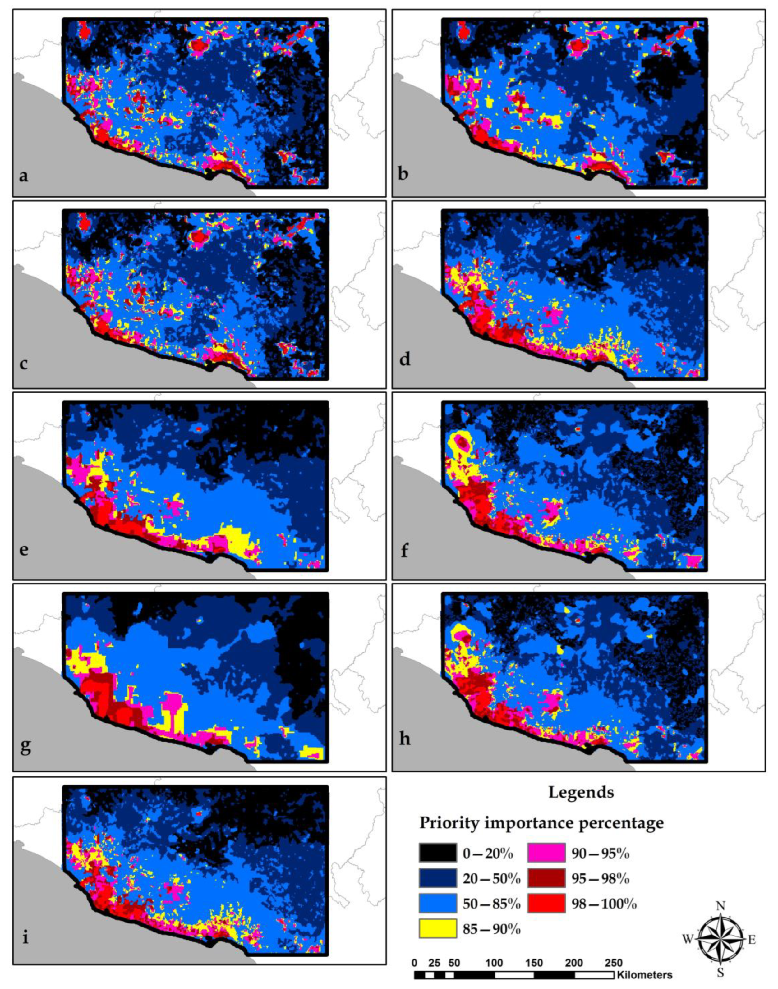
In general, each of the generated 18 models are located in the most important conservation areas within the western Michoacán coastal region. However, the models generated by applying the CAZ (core areas zoning) identified small highest priority areas towards the inland and northern sections of the study area (Figure A4).

The models generated in this study allow for flexibility in selecting different landscape area threshold percentages for conservation. For example, as shown in Figure A4, a 15% threshold percentage corresponds to the area in yellow, pink, cherry and red; a 5% threshold percentage corresponds to the areas in pink, cherry, and red, and finally, a 2% threshold percentage is represented by the areas in red (Figure A3).

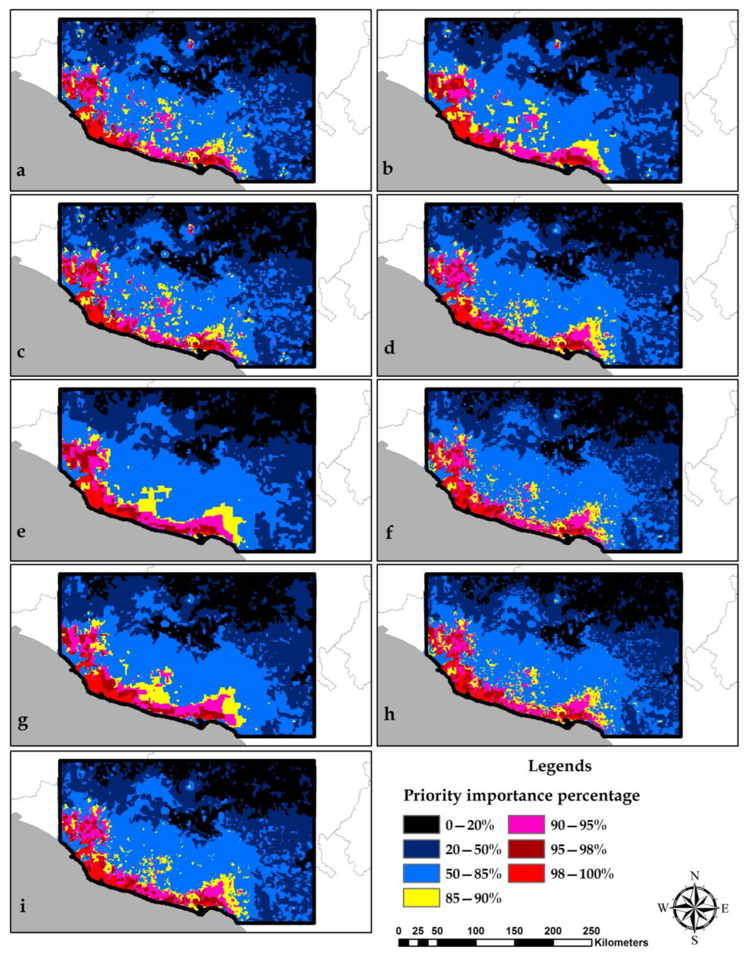
The two aggregation methods in the study resulted in small homogeneity differences in the models. In general, the BLP method tends to generalize and slightly increase the size of priority areas, reducing fragmentation, independently of the elimination rule. On the other hand, the smoothing method does not seem to significantly affect the priority areas’ spatial configuration (Figure A5).

The weights of species, depending on their conservation status, seem to have an apparent effect on the priority areas’ connection. Assigning a species’ weight generates a continuum in the coastal region, independently of the aggregation method and reduces the size of priority areas (the CAZ rule) located north of the study area (Figure A5).

The inclusion of the deforestation model does not significantly affect the identification of priority areas. The only apparent effect is the presence of a set of priority areas located in the northeastern study area (Figure A4a–c).

Despite these variations among the models, we found that all the models show a high concentration of high priority areas in the coastal region, which coincides with the species richness model, meaning, in other words, similar spatial patterns. These areas correspond to tropical forest formations, which show high vulnerability to degradation and fragmentation processes that occur in the region.

CONABIO et al. [49] identified 54 conservation priority hexagons (256 km² each) within the study area, with 10 being considered as high priority and 6 as extreme priority. Eight hexagons of high and extreme priority are distributed along the Michoacán coast, in correspondence with the high conservation priority areas identified by this study (2–15% percentage of landscape) (Figure 5).

4. Discussion

4.1. Modeling Scales

This study uses a two-scale approach for modeling the habitat suitability of carnivore species in western Michoacán. The large scale corresponded to western México, whose modeling was based on using climate prediction variables following the hypothesis that species distributions are primarily determined by this type of environmental factors at regional scales [84,85,86]. These models represent bioclimatic envelope models because climate and topography variables are used to build fundamental species ecological niches, which are projected to a geographic space [87]. The second scale consisted of western Michoacán; an area centered in the larger region, which is 1/5 of the size of the latter. This smaller area allowed for the collection of the current carnivore species occurrence data by means of applying a photo camera sampling method, and to perform land-use/land-cover change modeling, necessary data for generating actual species distribution models and applying analytical procedures for conservation planning and NPA network design [87,88].

4.2. Suitable Species Habitat Models

Previous studies have attempted to generate species distribution models from refining environmental envelope models in the field of conservation planning [87,89,90,91,92,93]; these have consisted of using a digitally documented suitable habitat map to intersect an environmental envelope model. In this study, this masking procedure is replaced by using a habitat/species associations model to restrict a bioclimatic envelope model. This model combination makes it possible to include the landscape’s habitat transformations in the climate/topography predicted model at local scales [94]. Indeed, the use of species/habitat-type associations, particularly on mammal species, has been supported in research on the use and selection of habitats that are widely abundant in ecological studies. Such studies apply statistical tests (e.g., logistic regression) to determine the levels of associations between species occurrence and habitat types [95,96,97]. However, these studies are conducted at local scales, limiting their application to conservation goals [98].

The GLM results showed that seven species had a significant variable that predicted species occurrences. This species occurrence probability is an objective and quantitative means to determine the levels of habitat suitability for each of the carnivore species. Four species that did not have significant predicting variables had the smallest occurrence sample size, which would be the first factor to be considered in explaining the GLM model performance [99,100,101].

The identification of suitable habitats where species are likely to occur has demonstrated to be a powerful conservation tool [102,103,104,105,106]. Moreover, this information is considered as a measurement of biodiversity units that serve as inputs for applying algorithms and geographic information systems (GIS) to identify priority conservation areas [92,107]. The efforts made towards prioritizing conservation areas in México have revealed the need to generate species distribution models at more reliable and finer scales [52].

The geographic description of most of this study’s carnivore species’ actual distribution models show similar spatial patterns as those described in the previously cited literature. On the other hand, this study’s habitat suitability models contrast with those distribution models proposed in studies with a national scope, such as the “Project DS006 Modeling mammal species distributions in México, a GAP approach” [108]; the former are significantly more restricted than the latter. For instance, even though Bassariscus astutus is reported to occur in most of Michoacán [109], and some historic records do exist [110,111], very few individuals have been recorded in the last two decades [58,112]. The Bassariscus astutus model showed the most restricted distribution among the 11 species (see Figure A3). The restricted nature of the previously mentioned habitat suitability models is closely related to the land-cover/land-use changes observed across the region [113]. A significant number of historic records related to Michoacán’s carnivore species are currently located in sites with agricultural and human settlement land uses [106].

4.3. Selection of Conservation Priority Areas

Different characteristics of biodiversity elements and the application of modeling tools and parameters affect the results in prioritization exercises for the selection and complementarity of conservation areas [81,114]. This study did not generate drastic changes when varying the zonation modeling parameters to identify conservation priority areas. There was a consensus for locating priority areas mainly in the Costas del Sur province and Cordillera Costera del Sur to a lesser extent. One important difference consisted of locating priority areas in the study area’s northern portion; when the prioritization rule was CAZ and with no species conservation status weighting, high priority areas appeared in “Pico de Tancíntaro” and “Volcán Nevado de Colima” NPA (Figure A4a–c).

There are two sanctuaries, “Playa de Maruata y Colola” and “Playa Mexiquillo”, which contain the highest priority importance areas (95–100%). These sanctuaries consist of very reduced areas (220 and 74 ha, respectively), with the original goal of protecting three species of marine turtles (Lepidochelys olivacea, Dermochelys coriacea, and Chelonia agassizii) [115,116]. Although these sanctuaries are marine NPAs, they can serve as a geographic reference for inland areas for biodiversity conservation.

The ZIBR attracts particular interest because of its location, biological diversity, endemism, size (265,000 ha) and legal status. The ZIBR is one of the largest biosphere reserves in México and was created in 2007. This NPA is occupied by high species richness (7–9 species), but has not been given the highest conservation importance priority status. However, this study’s results were obtained from a reduced number of species, and it is likely that other wider taxonomic groups would produce higher prioritization estimates within the ZIBR, based on the maximization of its biodiversity. This study used a group of umbrella species as indicators of biodiversity and could be considered as a preliminary approach for evaluating conservation priority areas [6,7].

The deforestation model in this study was inverted so that it represented the probability of natural areas to persist with their native land-cover type (Figure 4). Therefore, the prioritization procedure selected, with high prioritization importance, conserved areas of tropical dry forests, tropical semi-evergreen forests, and temperate forests. However, the prioritization procedure without the deforestation model resulted in the same selection of areas. This could be since both high species richness areas coincide with the areas of land-cover types with a high probability of persistence, given the land-cover/land-use changes that occurred between 1993 and 2014.

A comprehensive Marxan proposed prioritization study [49] was compared to this study’s results. Such a comprehensive study included the optimization analysis of 1450 biodiversity elements across México, including critical vegetation types, plant species at risk, the richness of plants and vertebrate species, resident birds, reptiles, amphibia, and mammals, along with 19 layers of threatening factors [49]. Despite the different scopes applied in each study, there were coincidences detected in the location of priority sites and areas. Our study included half of CONABIO’s high-priority conservation sites, which were included within the study area (Figure 5). In other words, both studies identify the Costas del Sur province in western Michoacán as an important region for the conservation of biodiversity. This kind of concurrence supports the idea that a small group of umbrella species may be used as biodiversity indicators, as biodiversity units are useful for prioritizing biodiversity conservation areas.

5. Study Limitations and Future Research

The main limitation of this study is the small sample sizes, particularly for the four carnivore species that occur in western Michoacán, despite the fact that photo-trap sampling was carried out for several months during the years 2010–2014. Such a small sample size resulted in the lack of robustness of some of the GLM models.

This study proposes the identification of conservation areas for 11 carnivore species distributed in western Michoacán, México, which represent the basis for further research on the following: (1) suitable sites to conduct species monitoring across the region; (2) conservation of Michoacán’s coastal region, mainly corresponding to the Aquila and Lázaro Cárdenas counties; (3) issues about the extent of the current proposed regions for biodiversity conservation, given their larger sizes and location; (4) connectivity of areas identified as a priority for biodiversity conservation; and (5) comparison of prioritization and complementarity exercises based on analyzing multiple taxonomic groups, including animal and plant taxa of different taxonomic hierarchy and functional groups, such as key and umbrella species.

6. Conclusions

Bioclimatic envelope models in western México and habitat/species associations in the western Michoacán state were combined to obtain habitat suitability models for 11 carnivore species distributed in western Michoacán. The habitat suitability models were considered as biodiversity units for identifying conservation areas for 11 species of carnivores. Natural protected areas (NPA) and the existing proposed conservation areas were spatially related to our identified conservation areas, highlighting the prioritization of Michoacán’s coastal region for biodiversity conservation. This study contributes a new method for refining environmental envelope models into actual habitat suitability models by including the actual landscape configuration, which has historically been severely modified. By using 11 carnivore species as biodiversity surrogates, we identified the priority conservation areas that have not been included in the current NPA system and have not been specifically selected by the existing conservation proposals. The high-priority conservation areas identified in this study spatially corresponded to the high-priority areas proposed by a national study that used multiple taxa and prediction variables. This study signifies a flexible basis from which future studies on planning and designing a network of natural protected areas can be carried out in the region.

References

- Cervantes-Zamora, Y.; Cornejo-Olgín, S.; Lucero-Márquez, R.; Espinoza-Rodríguez, J.; Miranda-Viquez, E.; Pineda-Velázquez, A. Provincias Fisiográficas de México; Comisión Nacional para el Conocimiento y Uso de la Biodiversidad: Tlalpan, Mexico, 2001. [Google Scholar]
- Bocco, G.; Mendoza, M.E.; Velázquez, A.; Torres, A. La Regionalización Geomorfológica Como Una Alternativa de Regionalización Ecológica En México: El Caso de Michoacán de Ocampo. Investig. Geográficas 1999, 40, 7–22. [Google Scholar] [CrossRef]
- Rzedowski, J. Diversidad y Orígenes de La Flora Fanerogámica de México. Acta Botánica Mex. 1991, 14, 3–21. [Google Scholar] [CrossRef] [Green Version]
- Villaseñor Gómez, L.; Leal Nares, O.A. La Biodiversidad En Michoacán: Estudio de Estado; Comisión Nacional para el Conocimiento y Uso de la Biodiversidad (CONABIO): Tlalpan, Mexico, 2005; ISBN 970-9000-28-4. [Google Scholar]
- Monterrubio-Rico, T.C.; Medellín, J.F.C.; Colín-Soto, C.Z.; Paniagua, L.L. Los Mamíferos de Michoacán. Rev. Mex. Mastozool. (Nueva Época) 2014, 4, 1–17. [Google Scholar]
- Gittleman, J.L.; Funk, S.M.; MacDonald, D.W.; Wayne, R.K. Carnivore Conservation; Cambridge University Press: Cambridge, UK, 2001; Volume 5. [Google Scholar]
- Ray, J.; Sunquist, M. Trophic Relations in a Community of African Rainforest Carnivores. Oecologia 2001, 127, 395–408. [Google Scholar] [CrossRef]
- Berger, J. Anthropogenic Extinction of Top Carnivores and Interspecific Animal Behaviour: Implications of the Rapid Decoupling of a Web Involving Wolves, Bears, Moose and Ravens. Proceedings of the Royal Society of London. Ser. B Biol. Sci. 1999, 266, 2261–2267. [Google Scholar] [CrossRef] [Green Version]
- Weber, W.; Rabinowitz, A. A Global Perspective on Large Carnivore Conservation. Conserv. Biol. 1996, 10, 1046–1054. [Google Scholar] [CrossRef]
- Wolf, C.; Ripple, W.J. Range Contractions of the World’s Large Carnivores. R. Soc. Open Sci. 2017, 4, 170052. [Google Scholar] [CrossRef] [Green Version]
- Ripple, W.J.; Estes, J.A.; Beschta, R.L.; Wilmers, C.C.; Ritchie, E.G.; Hebblewhite, M.; Berger, J.; Elmhagen, B.; Letnic, M.; Nelson, M.P.; et al. Status and Ecological Effects of the World’s Largest Carnivores. Science 2014, 343, 1241484. [Google Scholar] [CrossRef] [Green Version]
- Di Minin, E.; Slotow, R.; Hunter, L.T.B.; Montesino Pouzols, F.; Toivonen, T.; Verburg, P.H.; Leader-Williams, N.; Petracca, L.; Moilanen, A. Global Priorities for National Carnivore Conservation under Land Use Change. Sci. Rep. 2016, 6, 23814. [Google Scholar] [CrossRef] [Green Version]
- Ray, J.; Redford, K.H.; Steneck, R.; Berger, J. Large Carnivores and the Conservation of Biodiversity; Island Press: Washington, DC, USA, 2013; ISBN 978-1-59726-609-3. [Google Scholar]
- Terraube, J.; Van Doninck, J.; Helle, P.; Cabeza, M. Assessing the Effectiveness of a National Protected Area Network for Carnivore Conservation. Nat. Commun. 2020, 11, 2957. [Google Scholar] [CrossRef]
- Cardillo, M.; Purvis, A.; Sechrest, W.; Gittleman, J.L.; Bielby, J.; Mace, G.M. Human Population Density and Extinction Risk in the World’s Carnivores. PLOS Biology 2004, 2, e197. [Google Scholar] [CrossRef]
- Karanth, K.U.; Chellam, R. Carnivore Conservation at the Crossroads. Oryx 2009, 43, 1–2. [Google Scholar] [CrossRef] [Green Version]
- Franklin, J. Mapping Species Distributions: Spatial Inference and Prediction; Cambridge University Press: Cambridge, UK, 2010; ISBN 978-1-139-48529-6. [Google Scholar]
- Augustin, N.H.; Mugglestone, M.A.; Buckland, S.T. An Autologistic Model for the Spatial Distribution of Wildlife. J. Appl. Ecol. 1996, 33, 339–347. [Google Scholar] [CrossRef] [Green Version]
- Edwards, T.C., Jr.; Deshler, E.T.; Foster, D.; Moisen, G.G. Adequacy of Wildlife Habitat Relation Models for Estimating Spatial Distributions of Terrestrial Vertebrates. Conserv. Biol. 1996, 10, 263–270. [Google Scholar] [CrossRef]
- Brito, C.; Crespo, E.G.; Paulo, O.S. Modelling Wildlife Distributions: Logistic Multiple Regression vs. Overlap Analysis. Ecography 1999, 22, 251–260. [Google Scholar] [CrossRef]
- Manel, S.; Dias, J.M.; Buckton, S.T.; Ormerod, S.J. Alternative Methods for Predicting Species Distribution: An Illustration with Himalayan River Birds. J. Appl. Ecol. 1999, 36, 734–747. [Google Scholar] [CrossRef]
- Spitz, F.; Lek, S. Environmental Impact Prediction Using Neural Network Modelling. An Example in Wildlife Damage. J. Appl. Ecol. 1999, 36, 317–326. [Google Scholar] [CrossRef]
- Venier, L.A.; McKenney, D.W.; Wang, Y.; McKee, J. Models of Large-Scale Breeding-Bird Distribution as a Function of Macro-Climate in Ontario, Canada. J. Biogeogr. 1999, 26, 315–328. [Google Scholar] [CrossRef]
- Cowley, M.J.R.; Wilson, R.J.; León-Cortés, J.L.; Gutiérrez, D.; Bulman, C.R.; Thomas, C.D. Habitat-Based Statistical Models for Predicting the Spatial Distribution of Butterflies and Day-Flying Moths in a Fragmented Landscape. J. Appl. Ecol. 2000, 37, 60–72. [Google Scholar] [CrossRef]
- Jaberg, C.; Guisan, A. Modelling the Distribution of Bats in Relation to Landscape Structure in a Temperate Mountain Environment. J. Appl. Ecol. 2001, 38, 1169–1181. [Google Scholar] [CrossRef]
- Peterson, A.T. Predicting Species’ Geographic Distributions Based on Ecological Niche Modeling. Condor 2001, 103, 599–605. [Google Scholar] [CrossRef]
- Anderson, R.P.; Gómez-Laverde, M.; Peterson, A.T. Geographical Distributions of Spiny Pocket Mice in South America: Insights from Predictive Models. Glob. Ecol. Biogeogr. 2002, 11, 131–141. [Google Scholar] [CrossRef] [Green Version]
- Ball, L.; Peterson, A.; Cohoon, K. Predicting Distributions of Tropical Birds. Ibis 2002, 144, e27–e32. [Google Scholar]
- Vetaas, O.R. Realized and Potential Climate Niches: A Comparison of Four Rhododendron Tree Species. J. Biogeogr. 2002, 29, 545–554. [Google Scholar] [CrossRef]
- Guisan, A.; Hofer, U. Predicting Reptile Distributions at the Mesoscale: Relation to Climate and Topography. J. Biogeogr. 2003, 30, 1233–1243. [Google Scholar] [CrossRef] [Green Version]
- Elith, J.; Graham, C.H. Do They? How Do They? Why Do They Differ? On Finding Reasons for Differing Performances of Species Distribution Models. Ecography 2009, 32, 66–77. [Google Scholar] [CrossRef]
- Araújo, M.B.; New, M. Ensemble Forecasting of Species Distributions. Trends Ecol. Evol. 2007, 22, 42–47. [Google Scholar] [CrossRef]
- Peterson, A.T.; Soberón, J.; Pearson, R.G.; Anderson, R.P.; Martínez-Meyer, E.; Nakamura, M.; Araújo, M.B. Ecological Niches and Geographic Distributions (MPB-49); Princeton University Press: Princeton, NJ, USA, 2011; ISBN 978-0-691-13688-2. [Google Scholar]
- Peterson, A.T.; Soberón, J. Species Distribution Modeling and Ecological Niche Modeling: Getting the Concepts Right. Nat. Conserv. 2012, 10, 102–107. [Google Scholar] [CrossRef]
- Grinell, J. The Niche Relationship of California Thrsher. Auk 1917, 1, 64–82. [Google Scholar]
- Pressey, R.L. Ad Hoc Reservations: Forward or Backward Steps in Developing Representative Reserve Systems? Conserv. Biol. 1994, 8, 662–668. [Google Scholar] [CrossRef]
- Pressey, R.L.; Humphries, C.J.; Margules, C.R.; Vane-Wright, R.I.; Williams, P.H. Beyond Opportunism: Key Principles for Systematic Reserve Selection. Trends Ecol. Evol. 1993, 8, 124–128. [Google Scholar] [CrossRef]
- Cabeza, M.; Moilanen, A. Design of Reserve Networks and the Persistence of Biodiversity. Trends Ecol. Evol. 2001, 16, 242–248. [Google Scholar] [CrossRef]
- Prendergast, J.R.; Quinn, R.M.; Lawton, J.H. The Gaps between Theory and Practice in Selecting Nature Reserves. Conserv. Biol. 1999, 13, 484–492. [Google Scholar] [CrossRef]
- Stokland, J.N. Representativeness and Efficiency of Bird and Insect Conservation in Norwegian Boreal Forest Reserves. Conserv. Biol. 1997, 11, 101–111. [Google Scholar] [CrossRef]
- Pressey, R.L.; Possingham, H.P.; Day, J.R. Effectiveness of Alternative Heuristic Algorithms for Identifying Indicative Minimum Requirements for Conservation Reserves. Biol. Conserv. 1997, 80, 207–219. [Google Scholar] [CrossRef]
- Hopkinson, P.; Travis, J.M.J.; Prendergast, J.R.; Evans, J.; Gregory, R.D.; Telfer, M.G.; Williams, P.H. A Preliminary Assessment of the Contribution of Nature Reserves to Biodiversity Conservation in Great Britain. Anim. Conserv. Forum 2000, 3, 311–320. [Google Scholar] [CrossRef]
- Williams, P.; Gibbons, D.; Margules, C.; Rebelo, A.; Humphries, C.; Pressey, R. A Comparison of Richness Hotspots, Rarity Hotspots, and Complementary Areas for Conserving Diversity of British Birds. Conserv. Biol. 1996, 10, 155–174. [Google Scholar] [CrossRef]
- Margules, C.R.; Sarkar, S. Planeación Sistemática de La Conservación; UNAM-CONANP-CONABIO: Cuidad de México, México, 2009; ISBN 607-7607-12-6. [Google Scholar]
- Possingham, H.; Wilson, K.; Andelman, S.A.; Vynne, C.H. Protected Areas: Goals, Limitations, and Design. In Principles of Conservation Biology, 3rd ed.; Groom, M.J., Meffe, G.K., Carroll, R.C., Eds.; Sinauer Associates: Sunderland, MA, USA, 2006; pp. 507–549. ISBN 978-0-87893-518-5. [Google Scholar]
- Comisión Nacional de Áreas Naturales Protegidas (CONANP); Comisión Nacional de Áreas Naturales Protegidas (SIMEC). 2022. Available online: https://simec.conanp.gob.mx/ficha.php?anp=73®=11 (accessed on 21 March 2021).
- Arriaga Cabrera, L.; Espinoza Rodríguez, J.M.; Aguilar Zuñiga, C.; Martínez Romero, E.; Gómez Mendoza, L.; Loa Loza, E. Regiones Terrestres Prioritarias de México; Comisión Nacional para el Conocimiento y Uso de la Biodiversidad (CONABIO): Tlalpan, Mexico, 2000; ISBN 970-9000-16-0. [Google Scholar]
- Arizmendi, C.; Márquez-Valdemar, L. Áreas de Importancia Para La Conservación de Las Aves En México (AICA); CIPAMEX-CONABIO-CCN-FMCN: Mexico City, México, 2000. [Google Scholar]
- CONABIO (Comisión Nacional para el Conocimiento y Uso de la Biodiversidad); CONANP (Comisión Nacional de Áreas Naturales Protegidas); TNC (The Nature Conservancy Program México); PRONATURA (Pronatura, A.C.); FCF (Facultad de Ciencias Forestales); UANL (Universidad Autónoma de Nuevo León, México). Análisis de Vacíos y Omisiones En Conservación de La Biodiversidad Terrestre de México: Espacios y Especies. 2007. Ciudad de México, México. Available online: https://simec.conanp.gob.mx/pdf_evaluacion/terrestre.pdf (accessed on 23 April 2021).
- UMSNH-SEDUE Catálogo Selecto de La Biodiversidad de Michoacán; Gobierno del Estado–Secretaría de Desarrollo Urbano y Ecología: Chihuahua, Mexico, 1999.
- Velázquez, A.; Sosa, N.; Navarrete, J.A.; Torres, A. Bases Para La Conformación Del Sistema de Áreas de Conservación Del Estado de Michoacán; Secretaría de Urbanismo y Medio Ambiente, Universidad Nacional Autónoma de México: Mexico City, México, 2005; ISBN 978-970-703-329-0. [Google Scholar]
- Vázquez, L.; Bustamante–Rodríguez, C.; Arce, D.B. Area Selection for Conservation of Mexican Mammals. Anim. Biodivers. Conserv. 2009, 32, 29–39. [Google Scholar] [CrossRef]
- Álvarez-Solórzano, T.; López-Vidal, J. Biodiversidad de Los Mamíferos En El Estado de Michoacán; Instituto Politécnico Nacional. Escuela Nacional de Ciencias Biológicas. Base de Datos SNIB2010-CONABIO Proyecto: Ciudad de México, Mexico, 1998. [Google Scholar]
- Trejo, C.O.; Campillo, A.C.; Pulido, J.R. Mammals from the Tarascan Plateau, Michoacán, México. Rev. Mex. Mastozool. (Nueva Época) 1999, 4, 53–68. [Google Scholar] [CrossRef]
- Charre-Medellín, J.F. Uso de Manantiales Por Los Mamíferos Silvestres En Bosques Tropicales de Michoacán; Maestría Institucional en Ciencias Biológicas, Universidad Michoacana de San Nicolás de Hidalgo: Morelia, Michoacán, 2012. [Google Scholar]
- Monterrubio-Rico, T.C.; Charre-Medellín, J.F.; Villanueva-Hernández, A.I.; León-Paniagua, L. Nuevos registros de la martucha (Potos flavus) para Michoacán, México, que establecen su límite de distribución al norte por el Pacífico. Rev. Mex. Biodivers. 2013, 84, 1002–1006. [Google Scholar] [CrossRef] [Green Version]
- Charre-Medellín, J.F.; Monterrubio-Rico, T.C.; Botello, F.J.; León-Paniagua, L.; Núñez, R. FIRST RECORDS OF JAGUAR (Panthera onca) From the State of Michoacán, México. Southwest. Nat. 2013, 58, 264–268. [Google Scholar] [CrossRef]
- Urrea-Galeano, L.A.; Rojas-López, M.; Sánchez-Sánchez, L.; Ibarra-Manríquez, G. Registro de Puma yagouaroundi En La Reserva de La Biosfera Zicuirán-Infiernillo, Michoacán. Rev. Mex. Biodivers. 2016, 87, 548–551. [Google Scholar] [CrossRef] [Green Version]
- Ramamoorthy, T.; Bye, R.; Lot, A.; Fa, J. Biological Diversity of México: Origins and Distribution; Oxford University Press: Oxford, UK, 1993. [Google Scholar]
- Ramírez-Pulido, J.; Arroyo-Cabrales, J.; Castro-Campillo, A. Estado Actual y Relación Nomenclatural de Los Mamíferos Terrestres de México. Acta Zool. Mex. 2005, 21, 21–82. [Google Scholar] [CrossRef]
- Ramırez-Pulido, J.; González-Ruiz, N.; Gardner, A.; Arroyo-Cabrales, J. List of Recent Land Mammals of México. Special Publications of the Museum of Texas Tech University; Texas Tech University: Lubbock, TX, USA, 2014. [Google Scholar]
- Ceballos, G.; Arroyo-Cabrales, J.; Medellin, R.A.; Domínguez-Castellanos, Y. Lista Actualizada de Los Mamíferos de México. Rev. Mex. Mastozool. 2005, 9, 21–71. [Google Scholar]
- Ceballos, G.; Arroyo-Cabrales, J. Lista Actualizada de Los Mamíferos de México. Rev. Mex. Mastozool. Nueva Época 2013, 2, 27–80. [Google Scholar] [CrossRef]
- Guo, Q.; Liu, Y. ModEco: An Integrated Software Package for Ecological Niche Modeling. Ecography 2010, 33, 637–642. [Google Scholar] [CrossRef]
- Fick, S.E.; Hijmans, R.J. WorldClim 2: New 1-Km Spatial Resolution Climate Surfaces for Global Land Areas. Int. J. Climatol. 2017, 37, 4302–4315. [Google Scholar] [CrossRef]
- Phillips, S.J.; Dudík, M. Modeling of Species Distributions with Maxent: New Extensions and a Comprehensive Evaluation. Ecography 2008, 31, 161–175. [Google Scholar] [CrossRef]
- Elith, J.; Graham, C.H.; Anderson, R.P.; Dudík, M.; Ferrier, S.; Guisan, A.; Hijmans, R.J.; Huettmann, F.; Leathwick, J.R.; Lehmann, A.; et al. Novel Methods Improve Prediction of Species’ Distributions from Occurrence Data. Ecography 2006, 29, 129–151. [Google Scholar] [CrossRef] [Green Version]
- Phillips, S.J.; Dudík, M.; Elith, J.; Graham, C.H.; Lehmann, A.; Leathwick, J.; Ferrier, S. Sample Selection Bias and Presence-Only Distribution Models: Implications for Background and Pseudo-Absence Data. Ecol. Appl. 2009, 19, 181–197. [Google Scholar] [CrossRef] [Green Version]
- Hirzel, A.H.; Helfer, V.; Metral, F. Assessing Habitat-Suitability Models with a Virtual Species. Ecol. Model. 2001, 145, 111–121. [Google Scholar] [CrossRef] [Green Version]
- Zaniewski, A.E.; Lehmann, A.; Overton, J.M. Predicting Species Spatial Distributions Using Presence-Only Data: A Case Study of Native New Zealand Ferns. Ecol. Model. 2002, 157, 261–280. [Google Scholar] [CrossRef]
- Engler, R.; Guisan, A.; Rechsteiner, L. An Improved Approach for Predicting the Distribution of Rare and Endangered Species from Occurrence and Pseudo-Absence Data. J. Appl. Ecol. 2004, 41, 263–274. [Google Scholar] [CrossRef]
- Instituto Nacional de Estadística y Geografía, (INEGI). Carta de Uso Del Suelo y Vegetación, Serie V, Escala 1: 250,000; Instituto Nacional de Estadística y Geografía, (INEGI): Aguascalientes, Mexico, 2014. [Google Scholar]
- Instituto Nacional de Estadística y Geografía, (INEGI) Guía Para La Interpretación de Cartografía de Uso de Suelo y Vegetación: Escala 1:250,000: Serie V. 2014. Available online: https://www.inegi.org.mx/contenidos/temas/mapas/usosuelo/metadatos/guia_interusosuelov.pdf (accessed on 15 April 2020).
- Jenness, J. Topographic Position Index (Tpi_jen. Avx_extension for Arcview 3. x, v. 1.3 a, Jenness Enterprises [EB/OL]. 2006. Available online: http://www.jennessent.com/arcview/tpi.htm (accessed on 16 June 2021).
- Peterson, A.T.; Papeş, M.; Soberón, J. Rethinking Receiver Operating Characteristic Analysis Applications in Ecological Niche Modeling. Ecol. Model. 2008, 213, 63–72. [Google Scholar] [CrossRef]
- Osorio-Olvera, L. NicheToolbox: A Web Tool for Exploratory Data Analysis and Niche Modeling. 2016. Available online: http://shiny.conabio.gob.mx:3838/nichetoolb2/ (accessed on 3 March 2021).
- Instituto Nacional de Estadística y Geografía, (INEGI). Conjunto de Datos Vectoriales de La Carta de Uso Del Suelo y Vegetación. Escala 1:250 000. Serie II. Continuo Nacional 2001. Available online: https://www.inegi.org.mx/app/biblioteca/ficha.html?upc=702825007021 (accessed on 5 May 2020).
- Instituto Nacional de Estadística y Geografía, (INEGI). Conjunto de Datos Vectoriales de La Carta de Uso Del Suelo y Vegetación. Escala 1:250 000. Serie V. Conjunto Nacional 2013. Available online: https://www.inegi.org.mx/app/biblioteca/ficha.html?upc=702825007024 (accessed on 5 May 2020).
- Jiménez-Valverde, A.; Lobo, J.M. Threshold Criteria for Conversion of Probability of Species Presence to Either–or Presence–Absence. Acta Oecologica 2007, 31, 361–369. [Google Scholar] [CrossRef]
- Moilanen, A. Landscape Zonation, Benefit Functions and Target-Based Planning: Unifying Reserve Selection Strategies. Biol. Conserv. 2007, 134, 571–579. [Google Scholar] [CrossRef]
- Moilanen, A.; Anderson, B.J.; Eigenbrod, F.; Heinemeyer, A.; Roy, D.B.; Gillings, S.; Armsworth, P.R.; Gaston, K.J.; Thomas, C.D. Balancing Alternative Land Uses in Conservation Prioritization. Ecol. Appl. 2011, 21, 1419–1426. [Google Scholar] [CrossRef]
- Laitila, J.; Moilanen, A. Use of Many Low-Level Conservation Targets Reduces High-Level Conservation Performance. Ecol. Model. 2012, 247, 40–47. [Google Scholar] [CrossRef] [Green Version]
- Secretaría de Medio Ambiente y Recursos Naturales, (SEMARNAT). Norma Oficial Mexicana NOM-059-SEMARNAT-2010; Secretaría de Medio Ambiente y Recursos Naturales, Diario Oficial 30 Diciembre 2010: Distrito Federal, México, 2010. [Google Scholar]
- Soberón, J. Grinnellian and Eltonian Niches and Geographic Distributions of Species. Ecol. Lett. 2007, 10, 1115–1123. [Google Scholar] [CrossRef]
- Soberón, J.M. Niche and Area of Distribution Modeling: A Population Ecology Perspective. Ecography 2010, 33, 159–167. [Google Scholar] [CrossRef]
- Soberón, J.; Peterson, A.T. Interpretation of Models of Fundamental Ecological Niches and Species’ Distributional Areas. Biodivers. Inform. 2005, 2, 1–10. [Google Scholar] [CrossRef] [Green Version]
- Peterson, A.T. Uses and Requirements of Ecological Niche Models and Related Distributional Models. Biodivers. Inform. 2006, 3, 59–72. [Google Scholar] [CrossRef] [Green Version]
- Guisan, A.; Thuiller, W. Predicting Species Distribution: Offering More than Simple Habitat Models. Ecol. Lett. 2005, 8, 993–1009. [Google Scholar] [CrossRef] [PubMed]
- Sanchez-Cordero, V.; Munguia, M.; Peterson, A.T. GIS-Based Predictive Biogeography in the Context of Conservation. In Frontiers of Biogeography: New Directions in the Geography of the Nature; Lomolino, M.V., Heany, L.R., Eds.; Sinauer: Sunderland, MA, USA, 2004; pp. 311–324. [Google Scholar]
- Sánchez-Cordero, V.; Illoldi-Rangel, P.; Linaje, M.; Sarkar, S.; Peterson, A.T. Deforestation and Extant Distributions of Mexican Endemic Mammals. Biol. Conserv. 2005, 126, 465–473. [Google Scholar] [CrossRef]
- Sánchez-Cordero, V.; Illoldi-Rangel, P.; Escalante, T.; Figueroa, F.; Rodríguez, G.; Linaje, M. Deforestation and Biodiversity Conservation in México. In Endangered Species: New Research; Columbus, A., y Kuznetsov, L., Eds.; Nova Science Publishers: New Haven, CT, USA, 2009; pp. 279–298. [Google Scholar]
- Ortega-Huerta, M.A.; Peterson, A.T. Modelling Spatial Patterns of Biodiversity for Conservation Prioritization in North-Eastern México. Divers. Distrib. 2004, 10, 39–54. [Google Scholar] [CrossRef]
- Botello, F.; Sánchez-Cordero, V.; Ortega-Huerta, M.A. Disponibilidad de hábitats adecuados para especies de mamíferos a escalas regional (estado de Guerrero) y nacional (México). Rev. Mex. Biodivers. 2015, 86, 226–237. [Google Scholar] [CrossRef] [Green Version]
- Gillingham, P.K.; Palmer, S.C.F.; Huntley, B.; Kunin, W.E.; Chipperfield, J.D.; Thomas, C.D. The Relative Importance of Climate and Habitat in Determining the Distributions of Species at Different Spatial Scales: A Case Study with Ground Beetles in Great Britain. Ecography 2012, 35, 831–838. [Google Scholar] [CrossRef] [Green Version]
- Rodas-Trejo, J.; Rebolledo, G.; Rau, J. Uso y Selección de Hábitat Por Mamíferos Carnívoros y Herbívoros En Bosque Nativo y Plantaciones Forestales Del Sur de Chile. Gestión Ambient. 2010, 19, 33–46. [Google Scholar]
- Briceño-Méndez, M.; Reyna-Hurtado, R.; Calmé, S.; García-Gil, G. Preferenciasde hábitat y abundancia relativa de Tayassu pecari en un área con cacería en la región de Calakmul, Campeche, México. Rev. Mex. Biodivers. 2014, 85, 242–250. [Google Scholar] [CrossRef] [Green Version]
- Carrillo-Reyna, N.; Reyna-Hurtado, R.; Schmook, B. Abundancia relativa y selección de hábitat de Tapirus bairdii en las reservas de Calakmul y Balam Kú, Campeche, México. Rev. Mex. Biodivers. 2015, 86, 202–207. [Google Scholar] [CrossRef] [Green Version]
- Pinto-Ledezma, J.N.; Sandoval, X.V.; Pérez, V.N.; Caballero, T.J.; Mano, K.; Pinto Viveros, M.A.; Sosa, R. Desarrollo de un modelo espacial explícito de hábitat para la paraba jacinta (Anodorhynchus hyacinthinus) en el Pantanal boliviano (Santa Cruz, Bolivia). Ecol. Boliv. 2014, 49, 51–64. [Google Scholar]
- Hirzel, A.; Guisan, A. Which Is the Optimal Sampling Strategy for Habitat Suitability Modelling. Ecol. Model. 2002, 157, 331–341. [Google Scholar] [CrossRef]
- Reese, G.C.; Wilson, K.R.; Hoeting, J.A.; Flather, C.H. Factors Affecting Species Distribution Predictions: A Simulation Modeling Experiment. Ecol. Appl. 2005, 15, 554–564. [Google Scholar] [CrossRef] [Green Version]
- Wisz, M.S.; Hijmans, R.J.; Li, J.; Peterson, A.T.; Graham, C.H.; Guisan, A.; Group, N.P.S.D.W. Effects of Sample Size on the Performance of Species Distribution Models. Divers. Distrib. 2008, 14, 763–773. [Google Scholar] [CrossRef]
- Anderson, R.P.; Martínez-Meyer, E. Modeling Species’ Geographic Distributions for Preliminary Conservation Assessments: An Implementation with the Spiny Pocket Mice (Heteromys) of Ecuador. Biol. Conserv. 2004, 116, 167–179. [Google Scholar] [CrossRef]
- de la Torre, J.A.; Torres-Knoop, L. DISTRIBUCIÓN POTENCIAL DEL PUMA (Puma concolor) EN EL ESTADO DE AGUASCALIENTES, MÉXICO. Rev. Mex. Mastozool. (Nueva Época) 2014, 4, 45–56. [Google Scholar] [CrossRef] [Green Version]
- Torres, R.; Jayat, J.P. Modelos Predictivos de Distribución Para Cuatro Especies de Mamíferos (Cingulata, Artiodactyla y Rodentia) Típicas Del Chaco En Argentina. Mastozool. Neotrop. 2010, 17, 335–352. [Google Scholar]
- Cuervo-Robayo, A.P.; Monroy-Vilchis, O. Distribución potencial del jaguar Panthera onca (Carnivora: Felidae) en Guerrero, México: Persistencia de zonas para su conservación. Rev. Biol. Trop. 2012, 60, 1357–1367. [Google Scholar] [CrossRef] [Green Version]
- Charre-Medellín, J.F.; Monterrubio-Rico, T.C.; Guido-Lemus, D.; Mendoza, E.; Charre-Medellín, J.F.; Monterrubio-Rico, T.C.; Guido-Lemus, D.; Mendoza, E. Patrones de distribución de felinos silvestres (Carnívora: Felidae) en el trópico seco del Centro-Occidente de México. Rev. Biol. Trop. 2015, 63, 783–797. [Google Scholar] [CrossRef] [Green Version]
- Yañez-Arenas, C.; Peterson, A.T.; Mokondoko, P.; Rojas-Soto, O.; Martínez-Meyer, E. The Use of Ecological Niche Modeling to Infer Potential Risk Areas of Snakebite in the Mexican State of Veracruz. PLoS ONE 2014, 9, e100957. [Google Scholar] [CrossRef] [Green Version]
- Ceballos, G.; Blanco, S.; González, C.; Martínez, E. Modelado de La Distribución de Las Especies de Mamíferos de México Para Un Análisis GAP; Informe final SNIB-CONABIO proyecto DS006; EcoCiencia SC: Ciudad de México, México, 2008. [Google Scholar]
- Ceballos, G.; Oliva, G. Los Mamíferos Silvestres de México; CONABIO/Fondo de Cultura Económica: Mexico City, México, 2005. [Google Scholar]
- Nelson, E.W.; Goldman, E.A. Two New Cacomistles from México, with Remarks on the Genus Jentinkia. J. Wash. Acad. Sci. 1932, 22, 484–488. [Google Scholar]
- Burt, W.H. Some Effects of Volcan Paricutin on Vertebrates. Occasional Papers of the Museum of Zoology. Univ. Mich. 1961, 620, 1–24. [Google Scholar]
- Guido-Lemus, D. Riqueza de La Comunidad de Los Mamíferos Silvestres de La Cuenca Del Lago de Cuitzeo, Michoacán, Una Comparación Utilizando Métodos de Muestreo. Tesis de Licenciatura; Facultad de Biología, Universidad Michoacana de San Nicolás de Hidalgo: Morelia, Michoacán, México, 2012. [Google Scholar]
- Bocco, G.; Mendoza, M.; Masera, O. La Dinamica Del Cambio Del Uso de Suelo En Michoacán. Una Propuesta Metodológica Para el Estudio de Los Procesos de Deforestación; Instituto de Geografía-UNAM: Mexico City, México, 2001. [Google Scholar]
- Moilanen, A.; Franco, A.M.A.; Early, R.I.; Fox, R.; Wintle, B.; Thomas, C.D. Prioritizing Multiple-Use Landscapes for Conservation: Methods for Large Multi-Species Planning Problems. Proc. R. Soc. B Biol. Sci. 2005, 272, 1885–1891. [Google Scholar] [CrossRef] [PubMed] [Green Version]
- Comisión Nacional de Áreas Naturales Protegidas, (CONANP) CONANP 2018. Available online: https://simec.conanp.gob.mx/ficha.php?anp=47®=11 (accessed on 23 May 2021).
- Comisión Nacional de Áreas Naturales Protegidas, (CONANP) CONANP 2018. Available online: https://simec.conanp.gob.mx/ficha.php?anp=52®=11 (accessed on 23 May 2021).
- Coll-Hurtado, A. Nuevo Atlas Nacional de México; Universidad Nacional Autónoma de México: Mexico City, Mexico, 2007; ISBN 978-970-32-5047-9. [Google Scholar]
Figure 1.
Study areas’ location, physiographic provinces (see Table A1) and records of 11 carnivore species distributed in western México. (1) Delta del Río Grande de Santiago, (2) Sierras Neovolcánicas Nayaritas, (3) Altos de Jalisco, (4) Sierra de Jalisco, (5) Sierras de la Costa de Jalisco y Colima, (6) Guadalajara, (7) Chapala, (8) Sierras y Bajíos Michoacanos, (9) Mil Cumbres, (10) Neovolcánica Tarasca, (11) Cordillera Costera del Sur, (12) Volcanes de Colima, (13) Escarpa Limítrofe del Sur, (14) Depresión del Balsas, (15) Depresión de Tepalcatepec, (16) Sierras y Valles Guerrerenses, (17) Costas del Sur, and (18) Mesetas y Cañadas del Sur. Historical data are species occurrence records obtained from public collections, while recent occurrence data are records obtained from field sampling in western Michoacán.
Figure 2.
Natural protected areas (NPA) and existing proposed conservation regions and sites in western Michoacán, México. (A) NPA: (a) Zicuirán-Infiernillo biosphere reserve (ZIBR), (b) Pico de Tancintaro, (c) Volcán Nevado de Colima, (d) El Jabalí, (e) Las Huertas, (f) Lagunas Costeras y Serranias aledañas de la Costa de Michoacán, (g) El Barrancón de las Guacamayas, (h) Santuario Playa Maruata y Colola, (i) La Chichihua; (j) Santuario Playa Mexiquillo. (B) Terrestrial Priority Regions (TPR): (a) Infiernillo, (b) Sierra Coalcomán, (c) Tancíntaro, (d) Manantlán-Volcán de Colima; (e) Sierra Madre del Sur de Guerrero. (C) Important Areas for Bird Conservation (IABC): (a) Coalcomán-Pomaro, (b) Tumbiscatio, (c) Cuenca Baja del Balsas, (d) Vallecitos de Zaragoza, (e) Tacambaro, (f) Tancíntaro, (g) Patzcuaro; (h) Nevado de Colima. (D) Priority Terrestrial Sites for Biodiversity Conservation (PTSC). Polygons with black outlines are physiographic provinces.
Figure 3.
Flow diagram of the methods used. Dash lines separate two paths (scales), while boxes indicate the steps and obtained models.
Figure 4.
(A) Inverted deforestation, (B) species richness, and (C) topographic position index (TPI) models. Natural protected areas (NP): (a) Lagunas Costeras y Serranías Aledañas de la Costa Norte de Michoacán, (b) El Barrancón de las Guacamayas, (c) Santuario Playa Maruata y Colola, (d) Santuario Playa Mexiquillo, (e) Zicuirán-Infiernillo biosphere reserve, (f) Volcán Nevado de Colima; (g) Pico de Tancíntaro.
Figure 5.
Spatial correspondence between prioritization models and existing proposed priority terrestrial sites (PTSC; CONABIO et al., 2007) shown as hexagons. Black hexagons represent correspondence of highest conservation importance. (A): Prioritization model obtained by applying the additive benefit function (ABF), weighted species, the boundary length penalty (BLP), and the inverted deforestation model. (B) Prioritization model obtained by applying the core area zonation (CAZ) elimination rule and the same parameters as in model A.