
The Sensitivity of Micro—Macro Mechanical Behaviour of Sand to the Inter-Particle Properties


1
WSP, 3 Wellington Pl, Leeds LS1 4AP, UK
2
Faculty of Science and Engineering, School of Architecture and the Built Environment, University of Wolverhampton, Wolverhampton WV1 1LY, UK
3
School of Computer Science, University of Hull, Hull HU6 7RX, UK
*
Author to whom correspondence should be addressed.
Geotechnics 2023, 3(2), 416-445; https://doi.org/10.3390/geotechnics3020024
Submission received: 16 April 2023
/
Revised: 12 May 2023
/
Accepted: 17 May 2023
/
Published: 21 May 2023
(This article belongs to the Special Issue Multiscale and Multiphysics Modeling of Sub-Surface Geological Systems (2nd Edition))
Abstract
:Sand is a particulate material but is treated as a continuum solid in some engineering analyses. This approach is proven to be acceptable when dealing with geotechnical structures, provided an adequate factor of safety is applied so that there is no risk of failure. However, the continuum approach does not account for the effect of interparticle forces on the micro–macro behaviour of sand. Sand could be modelled as a particulate material using the discrete element method (DEM), taking into account its discrete nature. This paper shows how the microscopic contact properties between the idealised sand particles influence the macro-mechanical behaviour, highlighting the development of the fabric as the soil approaches failure. Thirty DEM biaxial tests were performed to study the sensitivity of the macro–micro mechanical properties of sand to the inter-particle properties of an idealised sand particle. The conditions of these simulations were the same (e.g., particle size distribution, number of particles, porosity after radius enlargement, boundary conditions, and rate of loading). The sensitivity of the pre-peak, peak, and post-peak behaviour of these simulations to the inter-particle properties of an idealised sand particle was studied. Two extra DEM biaxial tests under different confining pressures were performed to verify the cohesionless nature of the synthetic material used for this study. Since a two-dimensional DEM is used for this study, a detailed approach to interpret the results assuming either a plane strain or a plane stress situation was discussed. This study highlighted the critical inter-particle properties and the range over which these influence macro-mechanical behaviour. The results show that Young’s modulus is mainly dependent on the normal contact stiffness, and peak stress and the angle of internal friction are greatly dependent on the inter-particle coefficient of friction, while Poisson’s ratio and volumetric behaviour of particulate sand are dictated mainly by shear contact stiffness. A set of relationships were established between inter-particle properties and macro-machinal parameters such as Young’s modulus, Poisson’s ratio, and angle of internal friction. The elastoplastic parameters obtained from these tests are qualitatively in agreement with the typical medium and dense sand behaviour.
1. Introduction
The granular soil, such as sand, is consistently used in backfilling technologies, in particular in hydraulic backfilling, for which its compressibility is determined. The compressibility characteristics of sand are generally obtained from laboratory tests. These characterisations are then used in continuum models for geotechnical problems such as analyses of shallow and deep foundations, excavations, retaining walls, and slope stability. However, these models cannot account for the effect of microscopic inter-particle properties on the macroscale response of granular materials [1,2,3,4,5]. The bulk behaviour of sands is different from usual solid materials during shearing and presents a number of inter-particle interaction features, including anisotropy, nonlinear elasticity, dilatancy, state dependency, and non-coaxiality [6,7]. The complexity of the bulk behaviour of particulate sands mainly originates from their inter-particle properties and interactions of the constituent particles such that their macro-mechanical behaviours, including peak stress, angle of internal friction, Young’s modulus, and Poisson’s ratio, are inhibited by the interaction of inter-particle properties [7,8,9]. Interaction forces that develop during loading because of the inter-particle properties of individual particles create attributes such as fabric anisotropy. These critical features cannot be addressed in continuum mechanics [10,11]. Soil behaviour is stress-dependent [12,13,14], and ideal granular sand materials that have the same particle size distribution, density, and boundary conditions but varying inter-particle properties show different macro–micro behaviours at a certain macro stress level [15,16,17]. Research on the impact of inter-particle characteristics on the macro–micro responses of sands can improve our comprehensive understanding of the physical and mechanical properties of sands.
Alternatively, DEM can be used to simulate ideal granular systems. This is a proven and comprehensive method of studying granular soils [18,19,20,21,22]. The DEM model’s response is based on inter-particle forces and displacements, and the averaging method is used to obtain the average macro-mechanical response (e.g., Poisson’s ratio, Young’s modulus, angle of friction, peak stress, and others). The influence of inter-particle properties (e.g., normal and shear stiffness and inter-particle coefficient of friction) on the micro–macro response of particulate sand can be understood precisely through the DEM approach [23,24,25,26,27]. The macro-mechanical responses are normally validated against appropriate experimental data. The accuracy of this validation depends on the ability to replicate the geometric properties of the sample and choose the appropriate inter-particle properties. The former means creating a configuration of particles that has the same geometry, including boundary conditions and particle size distribution as the experimental sample. However, this cannot be achieved because of the nature of the particles; the number, shape, size, and distribution will be different between the numerical model and the experimental sample. Therefore, any model can be similar but not the same as the real sample. The second issue, and fundamentally more important, is the inter-particle relationship, which is based on a number of variables including the particle stiffness, particle size, and the inter-particle coefficient of friction, according to Zhao et al. [28]. It is possible to fit a single experimental curve with a number of combinations of these variables. However, not all combinations will be valid because there can be some interdependencies between the parameters, and there are limits to the range of the parameters.
A sensitivity analysis will identify the critical parameters and the range over which the parameters impact the mass behaviour. Bulk behaviour is used as the outcome as it provides a link to the experimental behaviour, which provides information on the macro mechanical properties. Many problems in geotechnical design assume plane strain [13,29]; therefore, a two-dimensional simulation is considered appropriate. The main objective of this study is to investigate the effect of these inter-particle parameters on the macro-mechanical parameters, including Young’s modulus, Poisson’s ratio, angle of internal friction, and the peak stress, and to identify the range over which the parameters impact the mass behaviour by performing Thirty DEM-based biaxial simulations. The effects of inter-particle parameters on the micro–macro parameters were parametrically investigated earlier (e.g., Mahmood and Iwashita [30]), and other notable parametric studies have been carried out by Belheine et al. [31] and Yang et al. [32]. They performed a series of 3D DEM triaxial tests using PFC3D [33] to calibrate their numerical model with experimental data. In that calibration study, they adjusted the slope of the stress–strain curve by changing normal contact stiffness values, while the slope of volumetric strain with axial strain was adjusted by the ratio of shear to normal contact stiffness. The calibration of peak stress was performed by changing in inter-particle coefficient of friction. A need to carry out sensitivity analysis is required to identify the critical inter-particle properties and the range over which these parameters impact the bulk behaviour. The sensitivity of macro–micro-mechanical properties of sand to the inter-particle properties are not yet explored comprehensively in the literature. This paper aims to study this gap using DEM by conducting a general framework for DEM simulation considering the 2D disk particle shape.
2. Two-Dimensional Simulations in DEM
The three-dimensional solution of a problem in continuum mechanics can be approximated by a two-dimensional solution (i.e., plane strain and plane stress) depending on the geometry of that problem, meaning the components of stress and strain tensors can be reduced to three components. To calculate stress and strain tensors within the particulate soil, an averaging method is used to estimate the average stress and strain tensors. That is, to compute the stress and strain tensors for a volume of particles within a two-dimensional DEM model using PFC2D, two in-plane force and displacement components and one in-plane moment are required. The out-of-plane force components and out-of-plane particle displacement are not taken into account in the motion equation—i.e., the out-of-plane forces and displacements which are essential to enforcing a state of plane strain or plane stress are not present. Therefore, the interpretation of 2D DEM results in terms of either plane strain or plane stress will be a controversial issue. Figure 1 displays a flowchart on two-dimensional used in DEM modellings.
Section 3 provides a more detailed explanation regarding the out-of-plane force component and out-of-plane particle displacement. The two-dimensional assumption, however, has an advantage. The dynamic response of a particulate system is greatly dependent on the number of degrees of freedom of each particle within these systems. In 3D DEM simulations, each idealised particle has six degrees of freedom, while in 2D cases, there are three degrees of freedom per particle. The computational effort in 2D DEM simulations will be less than in 3D simulations and, therefore, faster. Furthermore, the number of documented 2D DEM studies published annually shows that 2D DEM simulations are able to capture the key complex mechanical response features of soil medium [34,35,36]. Table 1 summarises the advantages and limitations of the use of 2D and 3D DEM modelling.
3. Plane Strain and Plane Stress Behaviour in DEM Simulations
For most geotechnical systems such as tunnels, retaining walls, earth dams, strip foundations, deep excavation, and slopes, soil behaviour is assumed to be dependent on the vector displacement field in two dimensions, and the effect of the vector displacement field in the third dimension is not very evident on the behaviour. This situation in continuum mechanics is called the plane strain, where a three-dimensional problem is analysed as a two-dimensional problem where values of the strain tensor components in the out-of-plane dimension are set to zero (i.e., ). In some cases, in continuum mechanics, the stress tensor field is also two-dimensional. In this case, the stress in the out-of-plane dimension is the intermediate stress. This situation is called plane stress. This does not apply in DEM analyses because no stress and strain tensor exist in such models. Instead, in two dimensions, only two in-plane force components and one in-plane moment are present (see Figure 1d). Section 4.1 presents the set of exemplary calculation formulas to calculate the two in-plane force components and one in-plane moment. In the averaging method, the average stress and strain tensors are computed. However, only the in-plane forces and displacements are used to calculate the average stress and strain tensors. The out-of-plane forces and displacements are not applied in calculating the average stress and strain tensors. Therefore, the out-of-plane constraint, which is essential to enforce a state of plane strain or plane stress, cannot be present. The formulations that describe plane stress and plane strain conditions will be explained, and the macro parameters (i.e., Elastic modulus, Poisson’s ratio, and angle of internal friction) obtained from these two situations are compared in order to assess the differences between both interpretations.
4. DEM Implementation in PFC2D
DEM is an advanced numerical tool originally proposed by Cundall and Strack [37]. It dynamically simulates and tracks the micro–macro-scale behaviour of granular materials subjected to quasi-static and dynamic loads. The central explicit finite difference scheme is used in this method to solve the dynamic equilibrium of each particle at each time step. In this paper, the DEM simulations are implemented using the software PFC2D 4.1 [38]. The rolling resistance is not adopted in this study. It has been experimentally observed by O’Sullivan et al. [39] that if the size of a particle is bigger than 0.1 (mm), the size of particle asperity will be negligible in comparison to the particle inertia. Therefore, the surface roughness will have a minor effect on the material behaviour in comparison to the particle inertia.
4.1. Contact Law
The contact force () applied on a disk particle in PFC2D code is decomposed into normal force () and tangential force (). The former is directed toward the particle centre, and the latter is directed along the tangent to the particle.
To preserve the geometry of particles during loading, it is assumed in PFC2D that particles are rigid with soft contact, which means that a contact overlap between two particles (e.g., a and b) is applied rather than a contact deformation. The magnitude of this overlap is computed by a contact law. In the present study, a linear elastic contact law is applied to calculate the components of contact forces. The normal and tangential displacements at time step are calculated as follows:
where , , , and are scalar translational and rotational particle velocities of particles a and b, respectively. and are the particle radius. and are the normal and tangential unit vectors.
The magnitude of the normal and tangential contact forces is calculated via the following:
The total contact shear force is compared to the Coulomb sliding friction or sliding capacity criterion (i.e., ) to check whether sliding has occurred. When the resultant force and torque in the z-direction (calculated by multiplying tangential contact force by the distance from the particle centre to the contact location) are computed for each particle, the local damping force will be added to them:
where , and are damping constant, resultant force on the particle, and particle velocity, respectively. The computed resultant force and torque acting on the particle are used to determine the change in particle velocity via Newton’s second law for the next time step. Once the resultant force is calculated for a particle, a damping force will be added to this at the end of each time step to reduce the kinetic energy of the particle. The damping force is calculated by multiplying a damping constant by the resultant force. The direction of the damping force is opposite to the particle velocity. The source of Equations (1)–(7) is [37,38].
4.2. Soil Fabric
In granular mechanics, soil fabric refers to the size, shape, and arrangement of soil particles. Fabric quantities include either particle orientation if 2D disk particles are used, or contact orientation and branch vector orientation for non-circular particles. These fabric quantities are often presented as an average or graphically (e.g., polar diagram of contacts). Rothenburg et al. [6] proposed a closed-form solution to estimate the polar diagram of contacts.
where represents “fabric anisotropy” in a granular system, depending on the number and density of unit normal vectors in principles axes. shows the deviation between the geometry of contact force distribution and the isotropic geometrical contact force distribution. For example, if , will be a circle such that the state of the system being considered is in an isotropic state. the direction of anisotropy. Parameters, are obtained by the following equations:
where is the total number of contact, , the number of segments and is the number of contacts within the th segment. In fact, the fabric anisotropy parameter shows the ability of granular systems to create the anisotropy state in normal contact distribution.
One of the key microscopic parameters, which are defined at the particle level, is the average coordination number which increases with densification [40,41]. This parameter is the average number of contacts per particle within a specific volume of a particulate assembly, and consequently, it provides a measure of packing density or packing intensity of fabric at the particle level. For a volume of particulate assembly with particles and total number of contacts, , the definition of average coordination number is given by the following:
4.3. The Typical Behaviour of Dry Sand
As schematically shown in Figure 2, the general macro–mechanical behaviour of sand subjected to the static deviatoric loading in a standard triaxial test is characterised by the following:
The initial Young’s modulus, E0 (the value of Young’s modulus at very small shear strains), is an important characteristic of soil deformability and plays an important role in the dynamic and static response of the soil. This is usually estimated by using laboratory or field tests that are related to seismic wave propagation and stiffness degradation curves based on cyclic tests conducted in the laboratory, which are costly, as shown by Okur and Ansal [43]. Where E0 is not available, E50, the secant modulus at 50% of peak stress, is often used to predict ground movements, as presented by Holtz et al. [44].
The slope of the volumetric strain vs. axial strain curve at a strain corresponding to half of the peak stress is used to compute Poisson’s ratio, ν, for both plane strain and plane stress.
In the case of dense and medium sand, the characteristic point, , corresponds to , where the dilation of the sample starts. The shear strain corresponding to this point varies between sands, as presented by Atkinson [14].
Small strains: Within this range, the stress–strain curve is assumed to be linear. In the case of dense and medium sand, the peak stress ratio or deviatoric stress occurs within this range.
Large strains: these correspond to strains exhibited when the soil is approaching failure, and the shear stiffness becomes small.
4.3.1. Elastic Parameters
In soil mechanics, it is assumed that at the start of a triaxial test, the material is linear elastic. In the principal stress space, the behaviour is as follows:
In terms of plane strain, the stress–strain relation is as follows:
In terms of plane stress, the stress–strain relation is as follows:
The elastic modulus and Poisson’s ratio are important characteristics when predicting ground movements, as it is often assumed that soil is isotropic and homogenous and behaves elastically. There are numerous methods available to determine these properties, but the most common is the triaxial test. In this test, using local strain measurements, it is possible to measure the stress–strain response of a sample of soil subjected to a variety of load paths (e.g., Head [45]). The values of stiffness obtained are stress path dependent and vary with the strain range over which they are measured. Stiffness is also a function of the confining stress, the particle geometry, and the density of packing. In this study, only monotonic compressive loading is monitored. Furthermore, the triaxial test is three-dimensional, whereas the DEM analysis used in this study is two-dimensional. However, since the soil is assumed to be isotropic and homogenous, the material properties obtained from the triaxial test can be applied to the two-dimensional analysis. In two-dimensional studies, it is necessary to consider plane stress or plane strain conditions, which lead to small differences in values of stiffness.
In plane strain situations, the secant Elastic modulus is as follows:
In a plane stress situation, the Elastic modulus is as follows:
When Poisson’s ratio is zero, the elastic modulus is equal for the plane stress and plane strain situations. Additionally, when Poisson’s ratio is 0.5, the elastic modulus in the plane strain is 75% of the elastic modulus in the plane stress [46].
Poisson’s ratio is obtained from the slope of the horizontal strain vs. axial strain curve. In two-dimensional analysis, the volumetric strain is In the plane stress condition, Poisson’s ratio is obtained from the following equation:
where is the horizontal strain and is the axial strain. In a plane strain situation, it is as follows:
4.3.2. Plastic Parameters
Angles of friction, , are related to the plastic and failure behaviour of non-cohesive material. For non-cohesive sand, the following relationship can be used to compute the angle of friction:
where t is the deviatoric stress and s is the isotropic stress.
4.4. The Methodology of Sensitivity Analysis
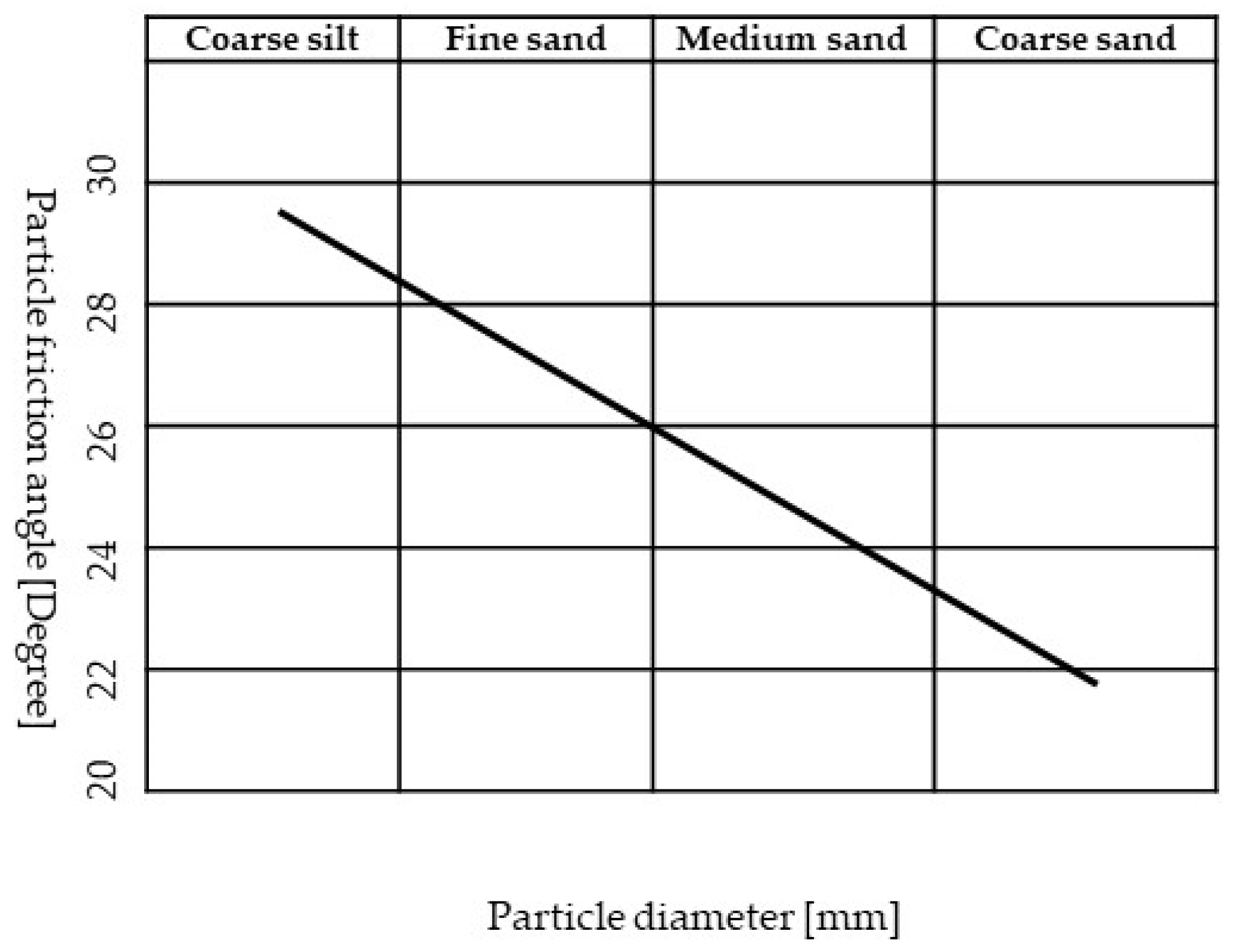
Three inter-particle properties, including normal and shear stiffness and inter-particle coefficient of friction, were considered in this research. Shear contact stiffness is presented as a ratio to normal stiffness. Values of the inter-particle properties of sand, including friction, normal, and shear contact stiffness, are listed in Figure 3 and Table 2.
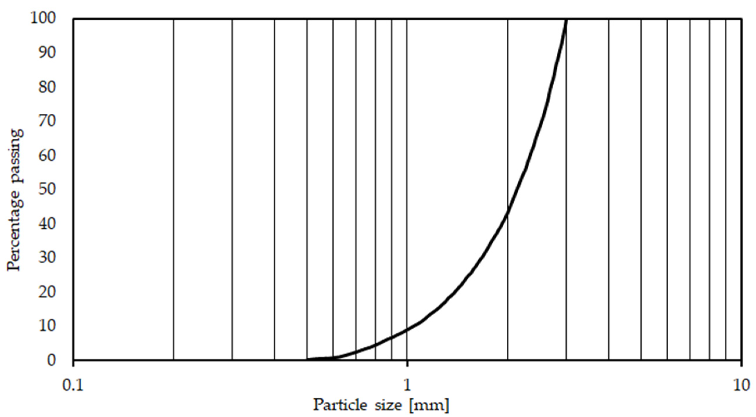
It was necessary to establish a methodology to measure the effect of inter-particle properties on the micro–macro mechanical behaviour of particulate idealised sand, expressed in terms of the angle of internal friction and stiffness of the sample. Each of the inter-particle properties was varied, keeping the others constant to determine the impact on the macro mechanical properties. The inter-particle properties for each biaxial test are obtained from Table 2. Table 3 summarises the input data used for this study. Figure 4 presents the particle size distribution profile used for this study.
Thirty biaxial tests in total were conducted to investigate the sensitivity of inter-particle properties on the micro–macro mechanical behaviour. The initial condition, such as the initial geometry of the biaxial chamber, particle size distribution, particle shape, contact model, porosity and isotropic stress state condition, and the lateral boundary condition for all these tests, were similar. Initially, non-overlapping disk particles in the range of 0.5 and 3 (mm) corresponding to the well grade of sand were randomly placed at half their size within four enclosed rigid walls. Their radii were then expanded to reach a porosity of 0.12. Next, the rigid boundaries of the biaxial cell were moved based on the applied strain control to approach the stress at the boundaries at 100 (kPa). Once the sample was isotopically consolidated to 100 (kPa), further cycles were needed to reach system equilibrium. It is to be noted that the porosity 0.12 mentioned in Table 2 is the porosity after radius enlargement. Next, the confining pressure on the vertical rigid boundaries was kept constant while the top and bottom rigid boundaries moved towards each other to apply deviatoric stress. The strain rate (i.e., ) applied for this test was , such that the incremental acceleration of each particle at each time step is small. All the imposed energy generated during the simulation was dissipated through both frictional sliding between particles and loss of contacts. In the sensitivity analysis, the critical parameters and the range over which the parameters impact the macro-mechanical behaviour are investigated. From each combination of normal stiffness, shear stiffness, and inter-particle coefficient of friction (i.e., ), the macro-mechanical parameters comprising Young’s modulus, Poisson’s ratio, and angle of internal friction were computed. These values will then be compared with typical values of elastic modulus, Poisson’s ratio, and angle of internal friction of sand obtained from the literature (see Table 4).
4.4.1. The Sensitivity of Sand System to the Inter-Particle Coefficient Friction
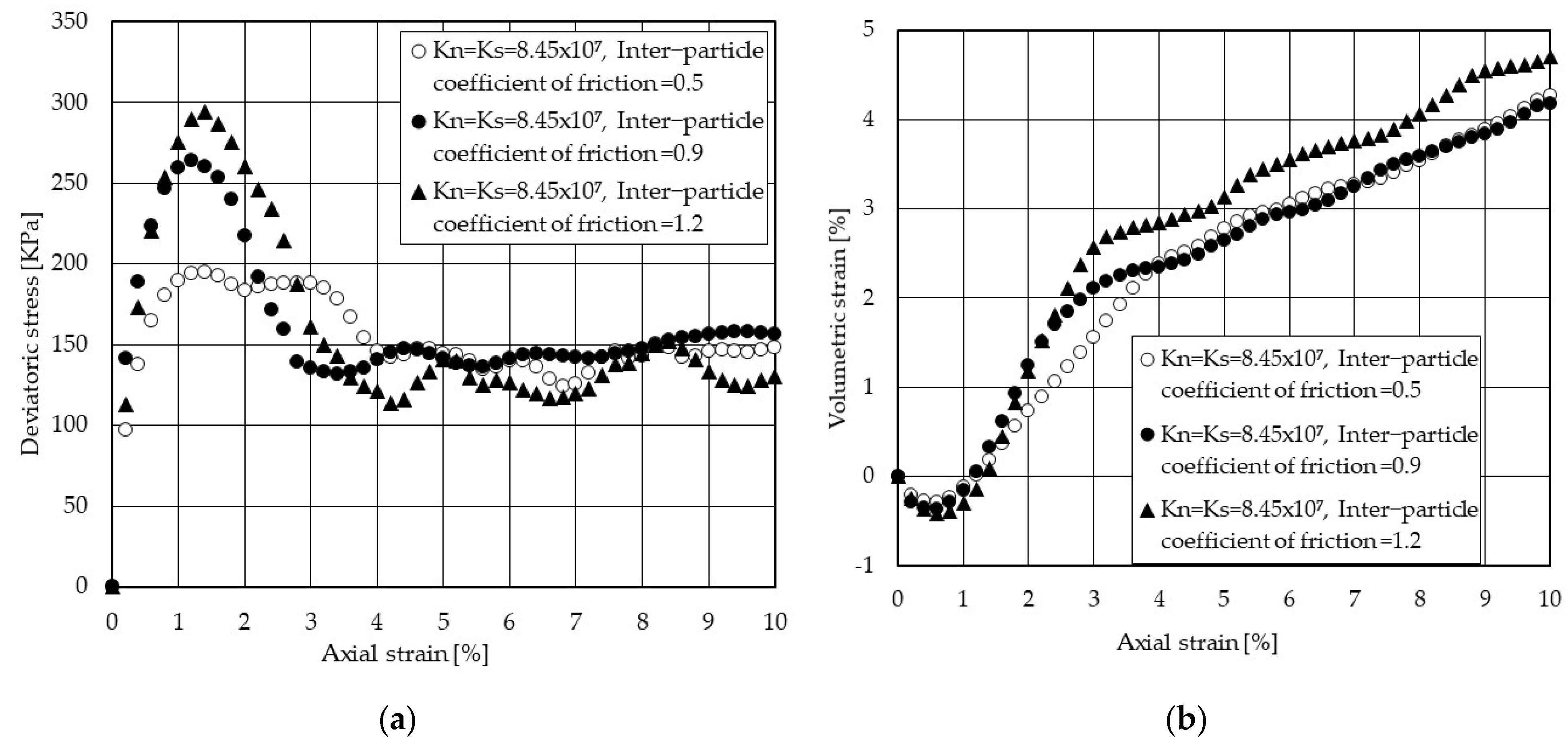
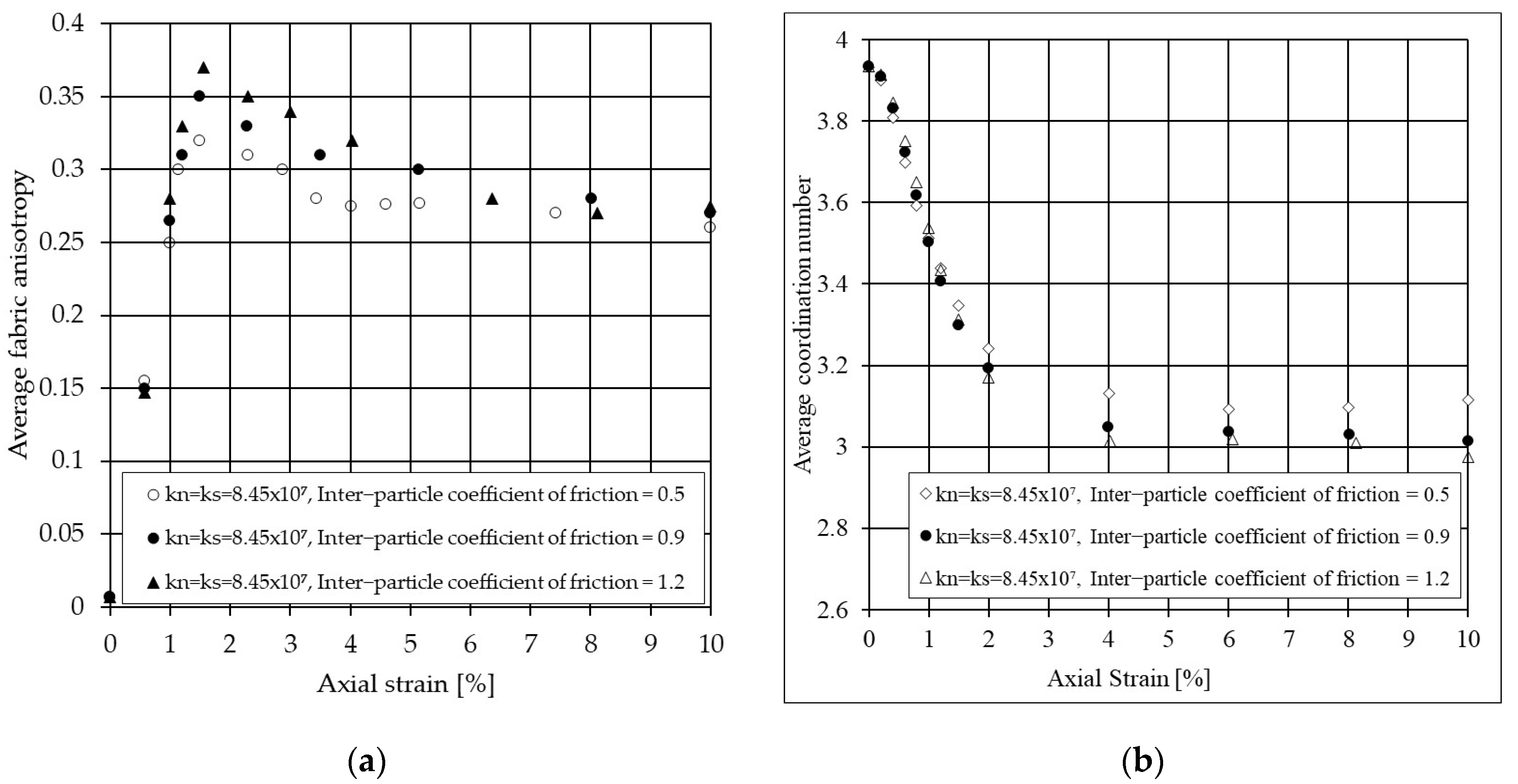
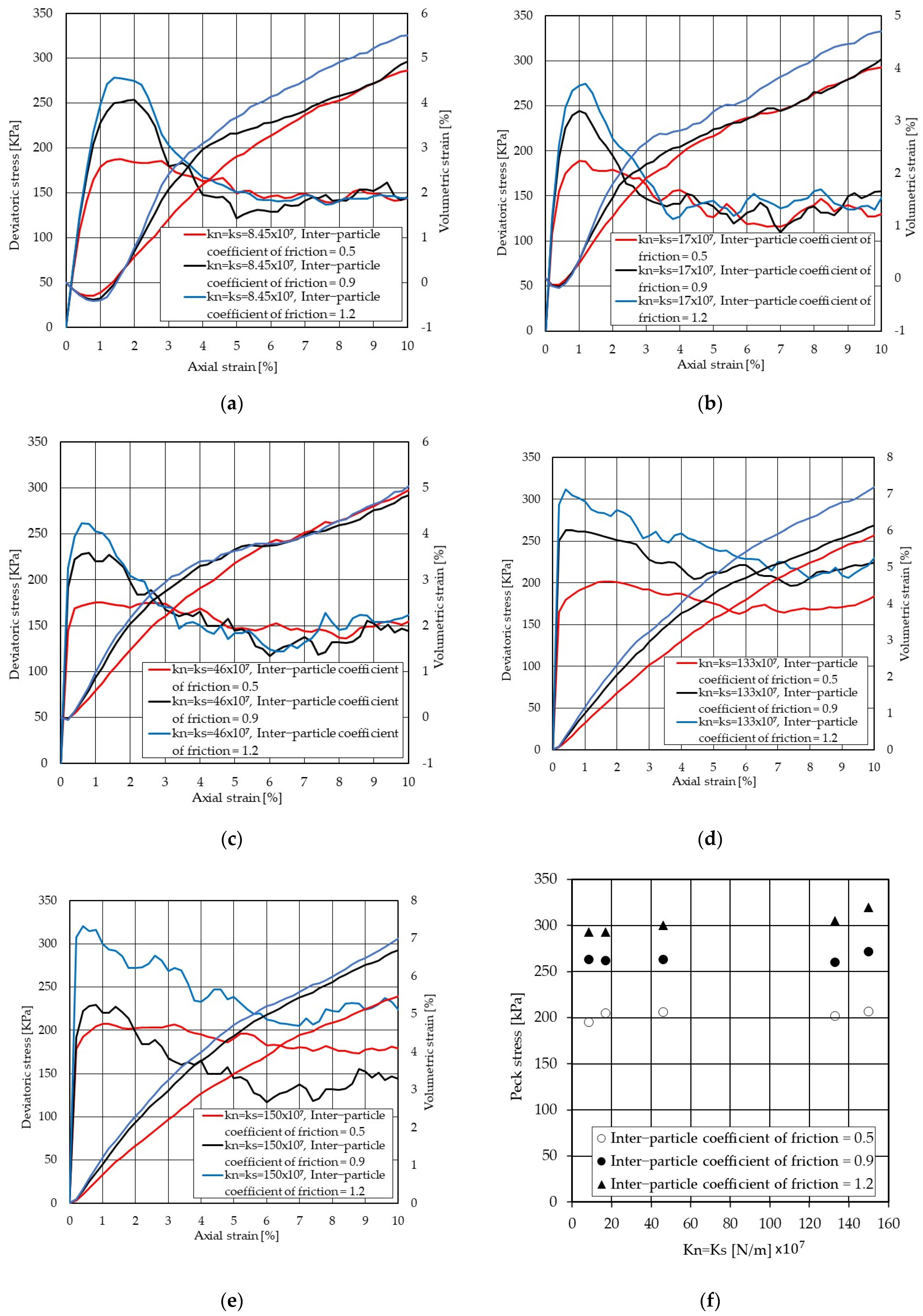
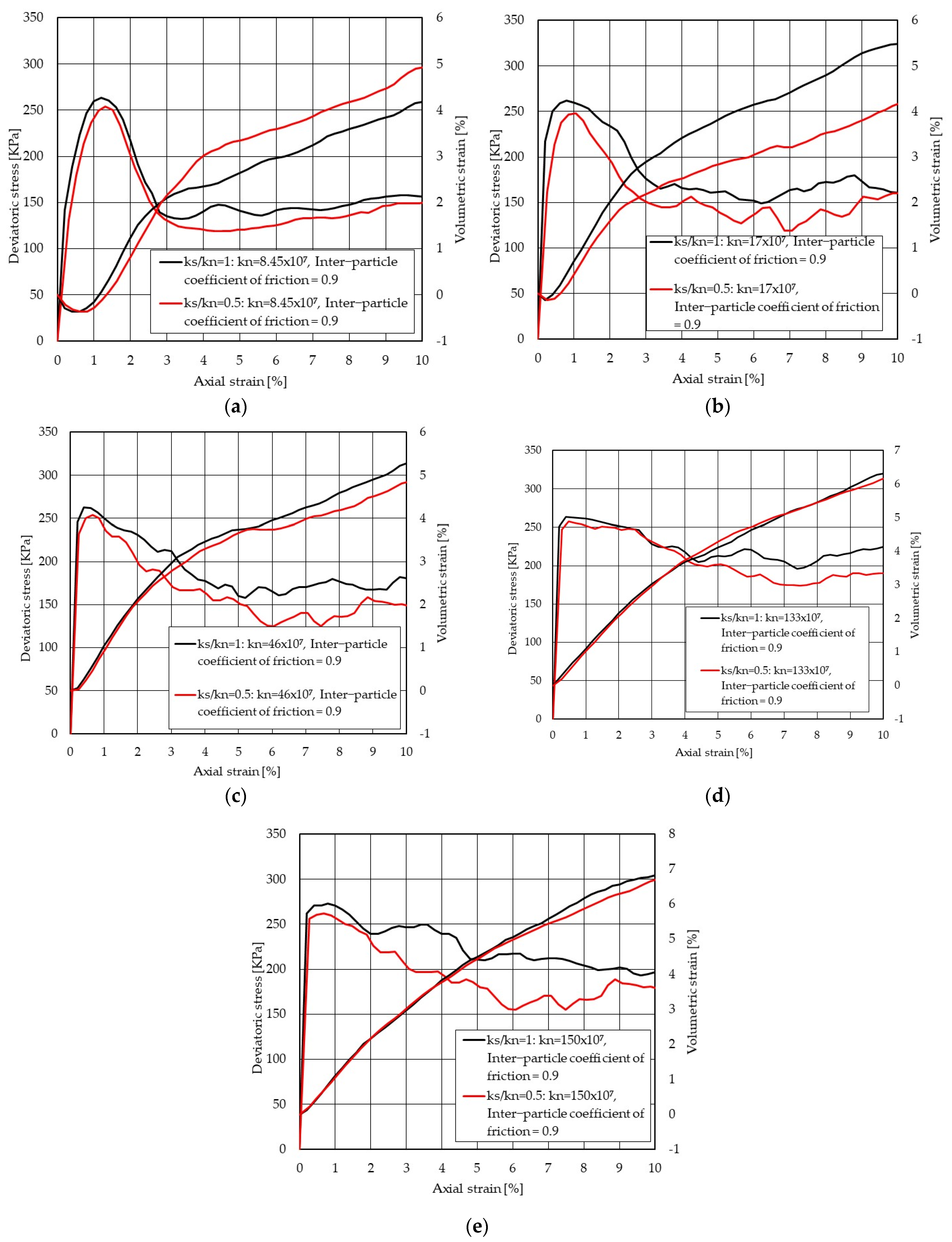
To investigate the sensitivity of the micro–macro-mechanical behaviour of particulate sand to the inter-particle coefficient friction, the ratio between normal contact stiffness and shear contact stiffness is assumed to be unity. By doing this, the number of biaxial tests required to be implemented was reduced to fifteen tests. The inter-particle properties used for these tests are listed in Table 5. Figure 5a illustrates the variations of deviatoric stress with axial strain for different inter-particle coefficients of friction where normal and shear contact stiffness is 8.45 × 10⁷ (N/m). As seen, for a fixed value of contact stiffness, the peak stress is profoundly controlled by inter-particle frictions, while the axial strain corresponding to the peak stress together with the slope of the stress–strain is less influenced by inter-particle frictions. Figure 5b shows that the contraction behaviour of particulate sand is less impacted by inter-particle frictions, though the model with bigger inter-particle coefficient friction (i.e., 1.2) shows slightly more dilative behaviour.
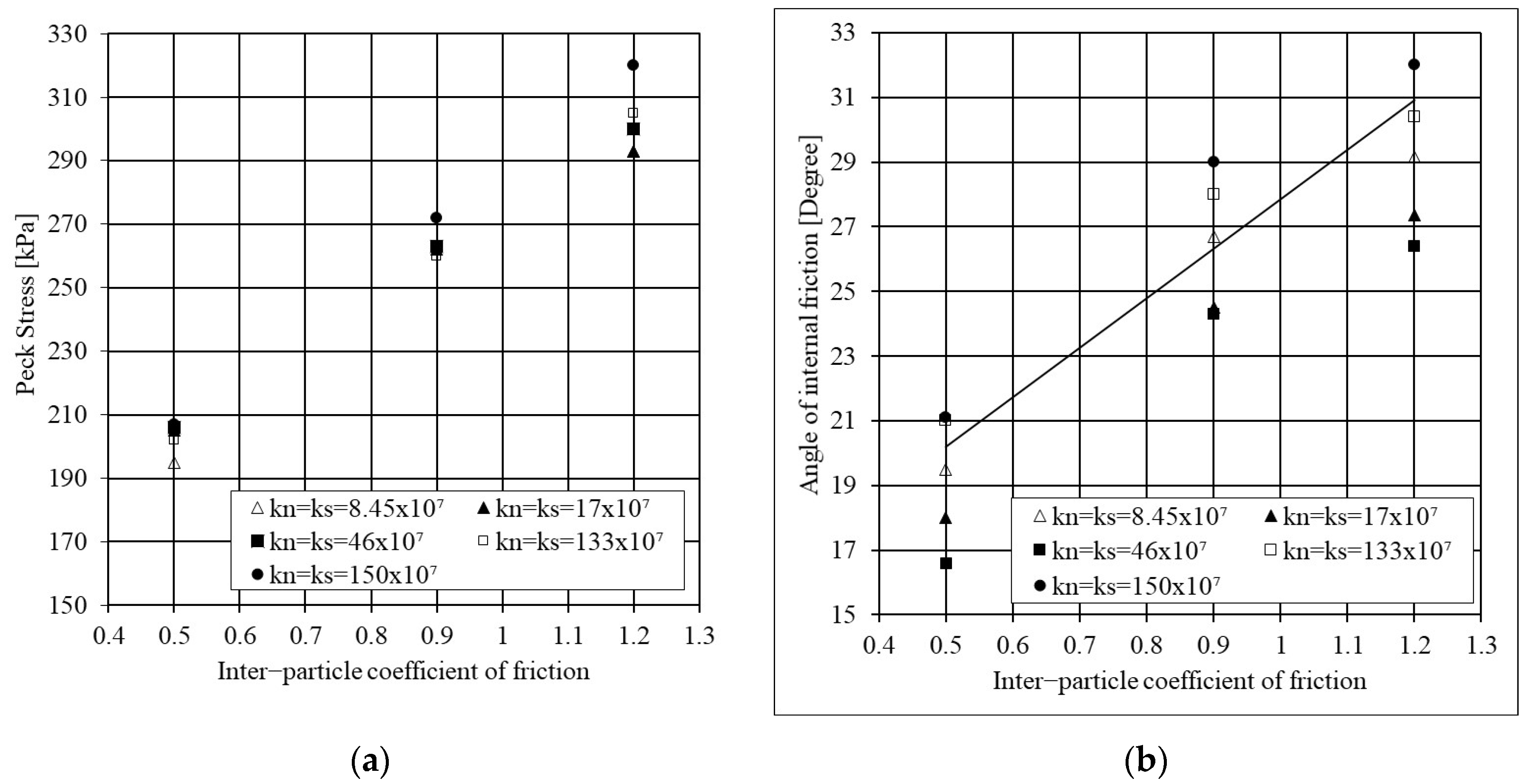
Figure 6a summarises the sensitivity of peak stress to the various inter-particle coefficient of friction for all these fifteen tests. As seen for each fixed value of contact stiffness, peak stress is significantly governed by inter-particle frictions. For example, for a fixed contact stiffness value of 8.45 × 10⁷ (N/m), changing the inter-particle coefficient of friction from 0.5 to 0.9 and 1.2 results in an increase in peak stress by 37% and 53%, respectively, resulting in an increase in the angle of internal friction from 20° to 26° and 29°, for the inter-particle coefficient of friction of 0.5 to 0.9 and 1.2, respectively (see Figure 6b). The angle of friction between 28° and 37° is typical for medium and dense sand. Based on the data provided for this study, a relationship between the inter-particle coefficient of friction and the angle of friction can be developed as follows:
where and are the angle of friction and inter-particle coefficient of friction. Note that this relationship is developed for inter-particle of coefficient between 0.5 and 1.2. It can be concluded that inter-particle friction mainly controls the peak stress and internal angle of friction.
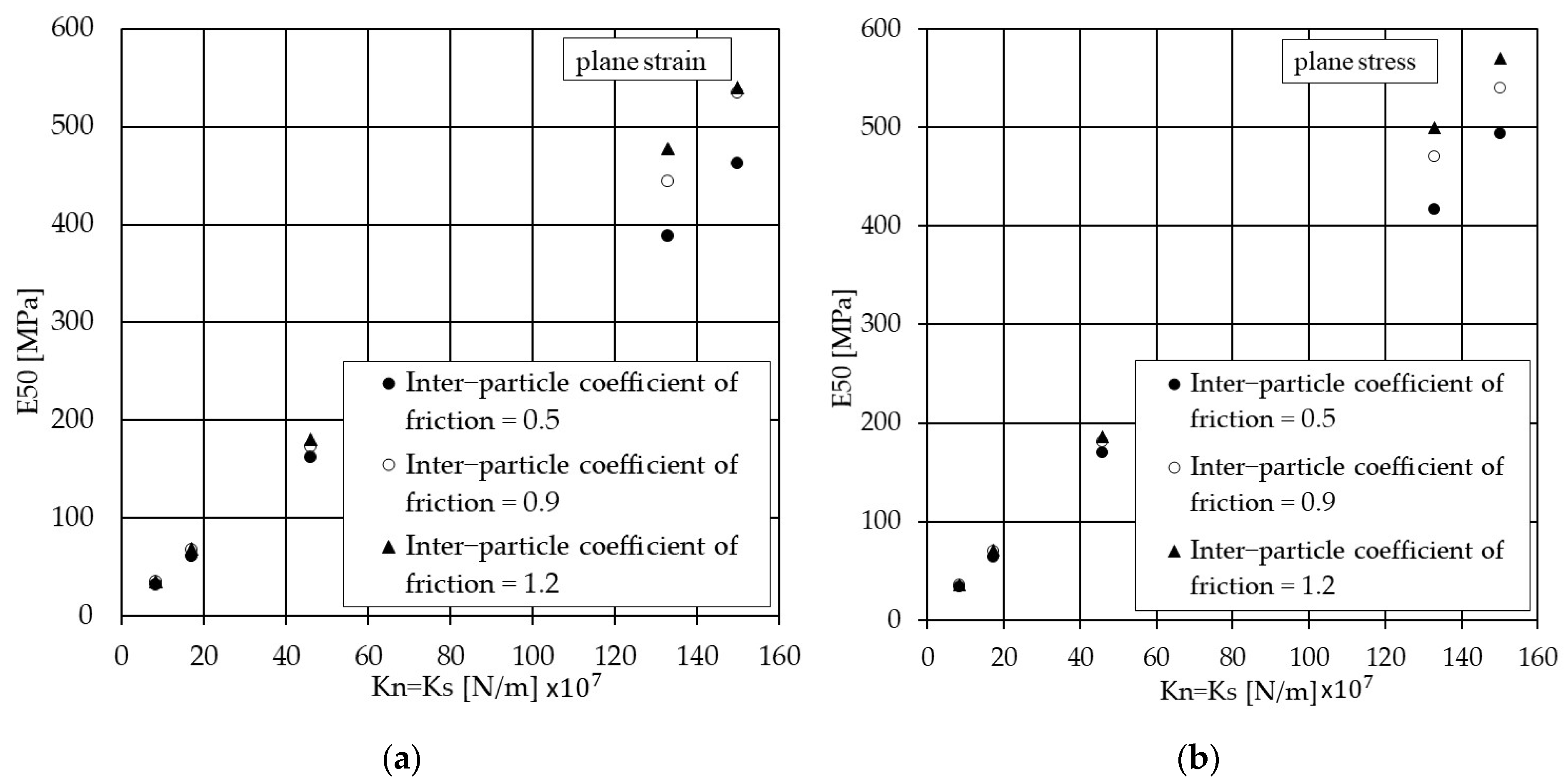
Table 6 summarises E50 with an inter-particle coefficient of friction for both plane stress and plane stress conditions, indicating that Young’s modulus is significantly governed by contact stiffness rather than the inter-particle coefficient of friction. For instance, changing the inter-particle coefficient of friction from 0.5 to 0.9 and 1.2 for a fixed contact stiffness value of 8.45 × 10⁷ (N/m), the plane strain E50 goes up by 8% and 0%, respectively. In the case of plane stress, E50 goes up by 5% and 0%, where the inter-particle coefficient friction changed from 0.5 to 0.9 and 1.2. Young’s modulus 25 (MPa) to 80 (MPa) is typical for medium and dense sand. Therefore, the contact stiffness above 17 × 107 (N/m) produces unrealistic Young’s modulus values.
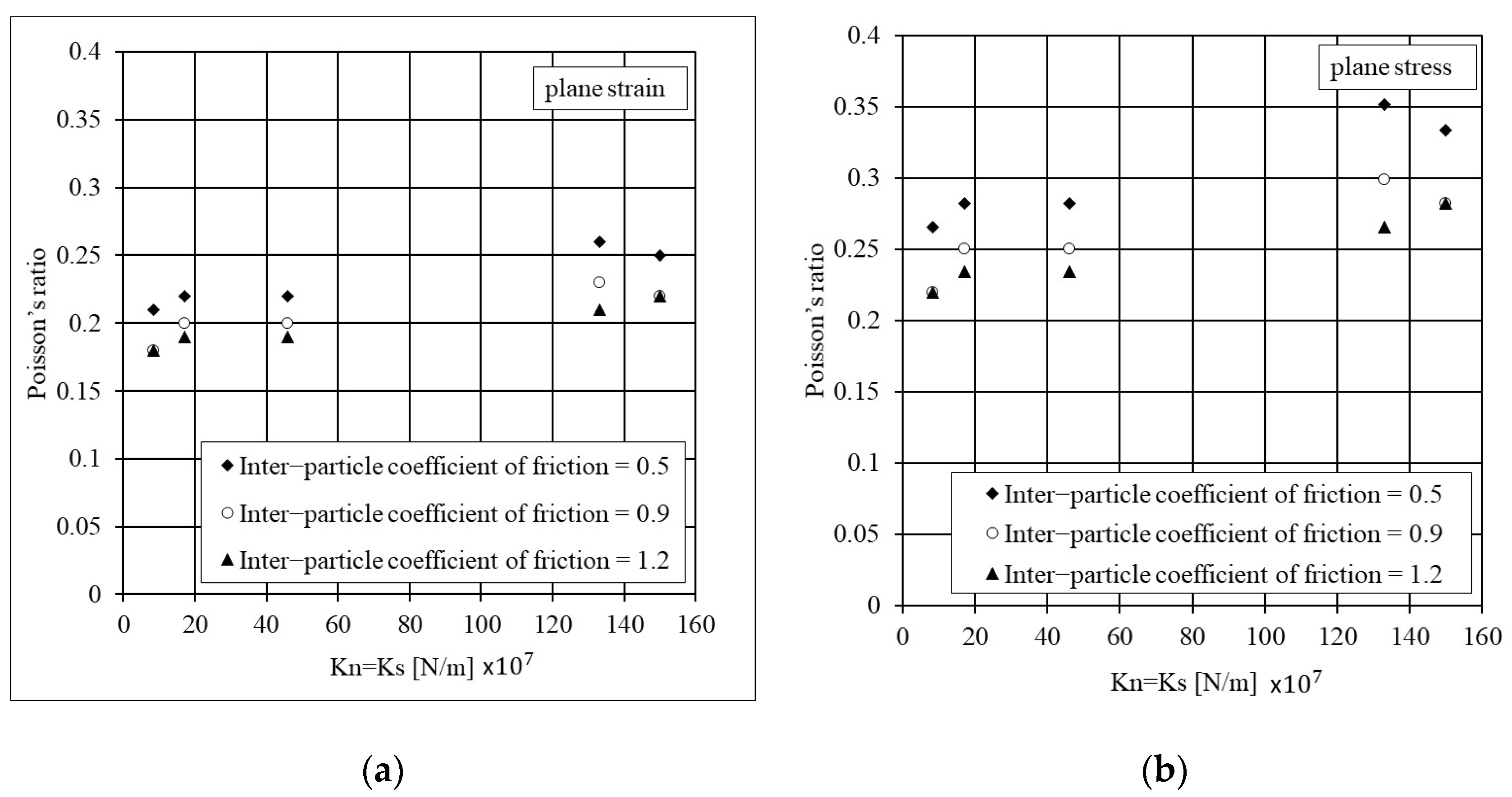
Table 7 shows that increasing the inter-particle coefficient of friction leads to an increase in Poisson’s ratio for both plane strain and plane stress conditions. However, the calculated Poisson’s ratio for plane stress is slightly greater than that calculated for plane strain. For instance, for inter-particle coefficient friction of 1.2 where the contact stiffness is 150 × 107 (N/m), the calculated Poisson’s ratio for plane strain and plane stress is 0.27 and 0.37, respectively. An increase in inter-particle coefficient friction leads to growth in both inter-particle sliding capacity and inter-particle forces, meaning the contact deformations and particle displacements rise. This leads to a rise in the lateral deformation of the system. The Poisson’s ratio between 0.2 and 0.3 is a typical value for medium and dense sand.
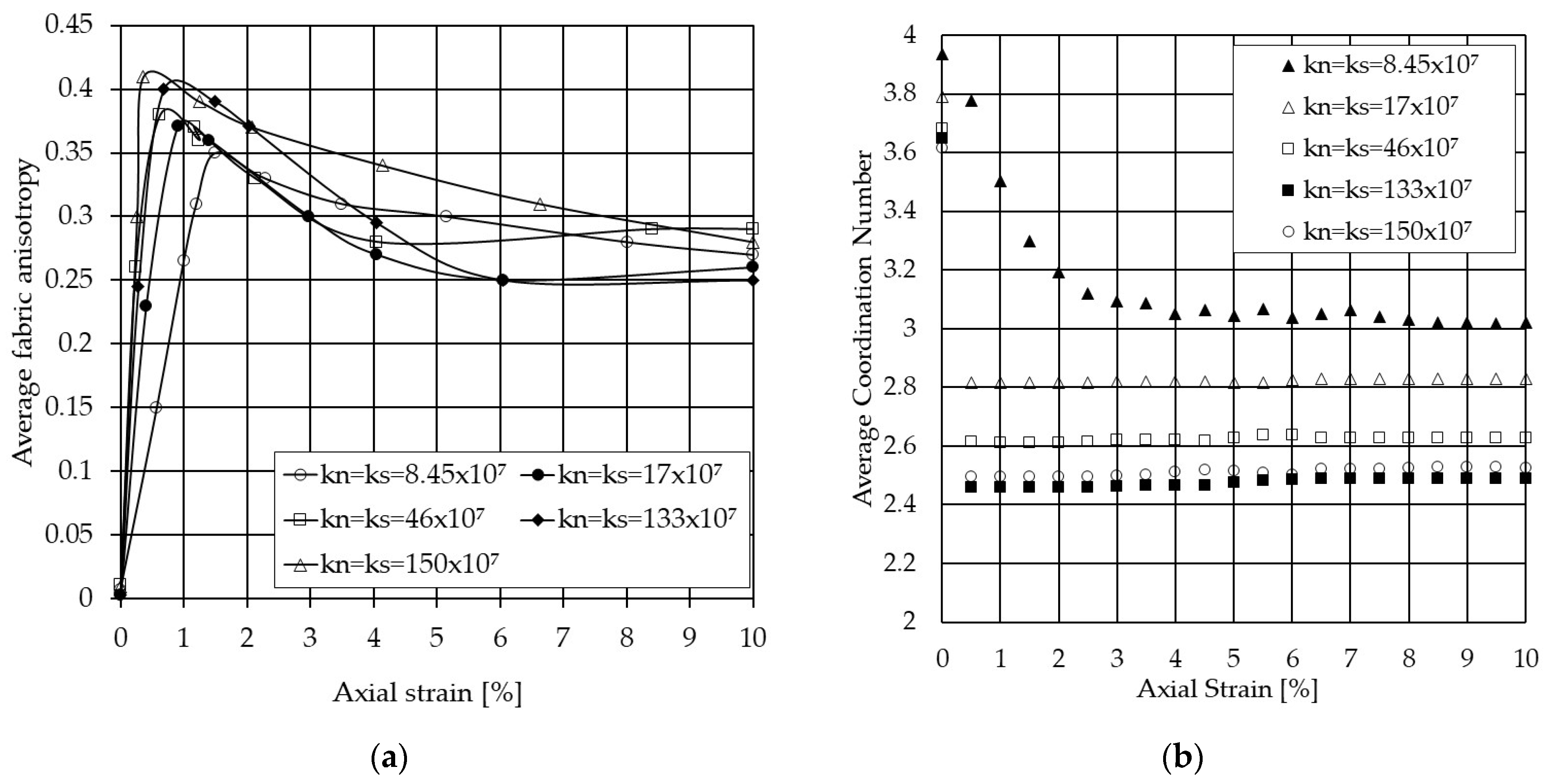
The trend of stress–strain behaviour presented in Figure 5a is in good agreement with average anisotropy with axial strain shown in Figure 7a. Figure 7a shows the average fabric anisotropy with axial strain to the various inter-particle coefficient of friction when a fixed value of contact stiffness is applied. The average fabric anisotropy increases until a maximum at the peak stress and then reduces with further strain for all inter-particle coefficients of friction. This clearly shows that the inter-particle coefficients of friction have a significant effect on the results. The maximum average fabric anisotropy, which is approximately 0.37, shows how much the contact arrangement drifts from the isotropic state (i.e., = 0). This term shows how much the system being loaded can develop anisotropy in contact networks. It is also a variance term that statistically shows how well the contact networks are changing during loading. The more average fabric anisotropy there is, the more shear strength capacity can be attained [6,8]. Figure 7b shows that an increase in the inter-particle coefficient of friction has little effect on the average coordination number to peak deviatoric stress up to the axial strain of 1.5%, which is representative of the peak deviatoric stress (refer to Figure 5a). The coordination number is then slightly increased though the value depends on the inter-particle coefficient of friction.
4.4.2. The Sensitivity of Sand System to Normal Contact Stiffness
A series of 15 biaxial tests were performed to determine the effect of the normal contact stiffness on the micro–macro properties of the particulate sand samples. The input data for these 15 tests are listed in Table 5. The ratio between normal contact stiffness and shear contact stiffness is assumed to be unity, while the inter-particle coefficient of friction varies between 0.5, 0.9, and 1.2. The sensitivity of combined deviatoric stress and volumetric strain with axial strain for a wide range of contact stiffness values is presented in Figure 8. It can be seen that the axial strain corresponding to the peak stress notably becomes smaller by increasing the contact stiffness, showing the particulate sand system behaves denser. However, the particulate systems with the lower contact stiffness demonstrate more softening strain behaviour at post-peak, while the particulate systems with higher contact stiffness show more hardening strain behaviour up the peak stress. Additionally, the peak stress for higher values of contact stiffness becomes sharper. Figure 8 also summarises the sensitivity of peak stress to the various normal contact stiffnesses and inter-particle coefficients of friction. Increasing the contact stiffness has less impact on the peak deviatoric stress. For instance, an increase in the normal contact stiffness from 8.45 × 10⁷ (N/m) to 150 × 107 (N/m), where a fixed value of the inter-particle coefficient of friction 0.9 is applied, results in a slight increase to the peak stress by about 2%. Figure 8 shows that the particulate sand system with the lower value of contact stiffness (e.g., 8.45 × 10⁷ (N/m) and 17 × 107 (N/m)) demonstrates more contraction behaviour due to the shearing followed by dilation behaviour, which is similar to the normal volumetric bulk behaviour of medium and dense sand. In contrast, the model with a higher value of contact stiffness (e.g., 47 × 107 to 150 × 107 (N/m)) demonstrates notable dilation behaviour with small initial contraction.
As highlighted in Figure 8, an increase in contact stiffness results in the slope of deviatoric stress with axial strain becoming steeper, meaning the bulk stiffness of particulate sand rises. It is because the increase in contact stiffness value and inter-particle friction leads to an increase in the sliding capacity of the contacts. That is, the risk of losing the contacts per particle reduces, and the number of contacts contributing to taking the load is high. Figure 9 and Table 6 show the plane stress and plane strain secant elastic modulus of the particulate sand systems for a wide range of contact stiffness and inter-particle coefficient of friction. A linear relationship can be established for each inter-particle coefficient of friction. In the case of plane strain,
In the case of plane stress, another set of linear relationships can be established for each inter-particle coefficient of friction:
The values of normal contact stiffness between 8.45 × 10⁷ (N/m) and 17 × 107 (N/m) lead to values of E50, which fall within the range typical for medium and dense sand, i.e., between 25 (MPa) and 50 (MPa) and 50 (MPa) and 80 (MPa), respectively.
Figure 10 and Table 7 show that an increase in the normal contact stiffness leads to an increase in Poisson’s ratio with a ranged value between 0.2 and 0.4. The contact stiffness of particles between 8.45 × 10⁷ (N/m) and 17 × 107 (N/m) produces typically ranged values of Poisson’s ratio for medium sand if the inter-particle coefficient of friction is between 0.9 and 0.5. For the higher value of the inter-particle coefficient of friction (i.e., 1.2), the interpreted value of Poisson’s ratio is less than typical values. A linear relationship can also be established between Poisson’s ratio and the inter-particle coefficient of friction (in the case of plane strain):
A linear relationship can also be established between Poisson’s ratio and the inter-particle coefficient of friction (in the case of plane stress):
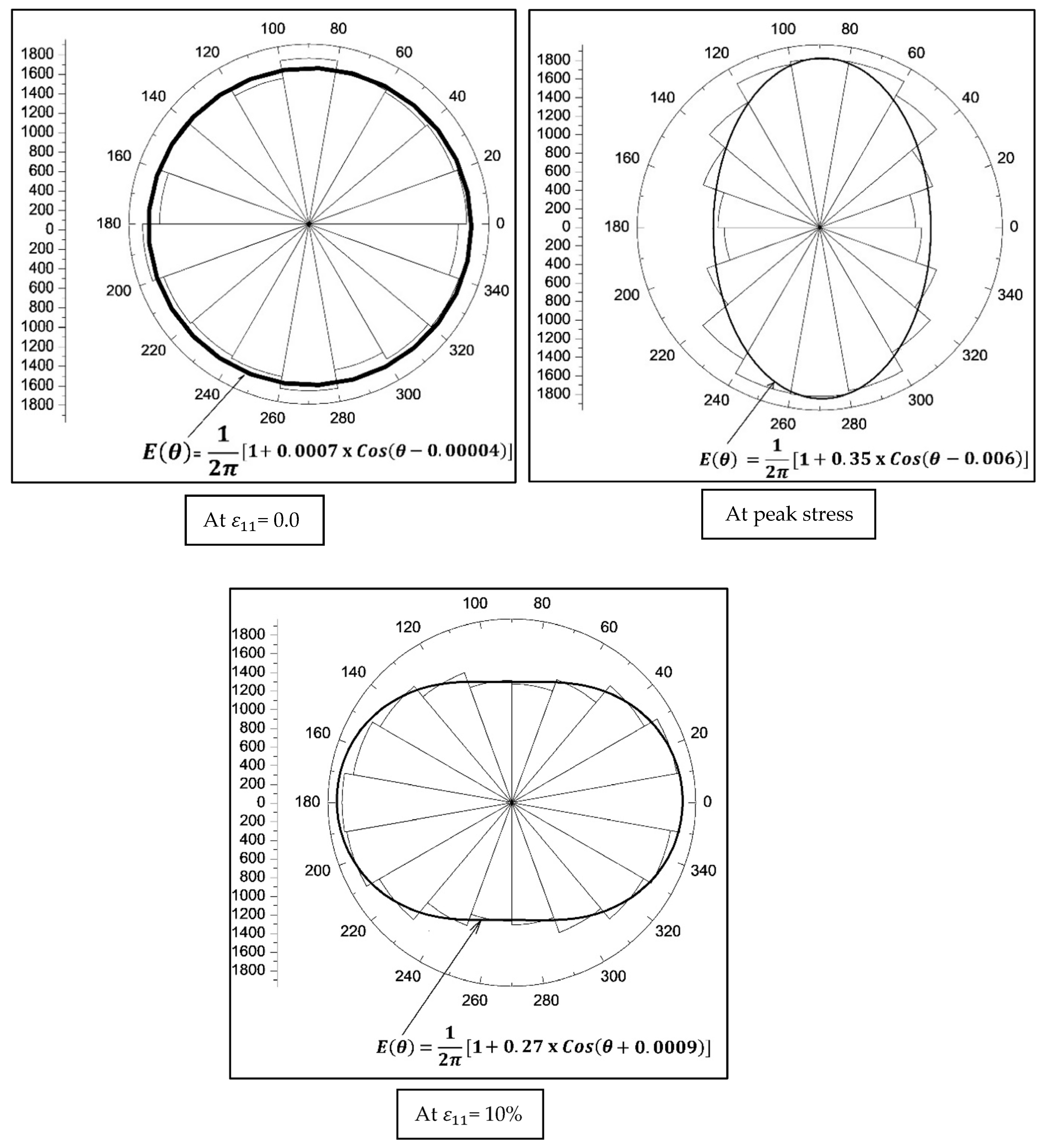
Figure 11 demonstrates the evolution of contact distribution during the shearing of particulate and where a fixed value is applied to the inter-particle properties. At this isotropic state, the average fabric anisotropy is 0.0007, and a circle presents the polar diagram distribution of contacts. At this stage, the number of contacts is distributed almost equally within each segment. If the polar diagram is entirely circled, it shows that the distribution of contacts is in an isotropic state. At the peak bulk deviatoric stress, the orientation of the contacts will be toward the direction of major stress, indicating the contacts within the particulate sand are fully mobilised to take the load. The average fabric anisotropy rises to 0.35. At the post-peak state where = 10%, the orientation of contact points will be mainly toward the confining stress, and average fabric anisotropy will be reduced to 0.27, showing the particulate system has collapsed.
An increase in contact stiffness from 8.45 × 10⁷ (N/m) to 150 × 107 (N/m) leads to an increase in average fabric anisotropy (see Figure 12a). Raising the ability of particulate systems to develop the fabric anisotropies results in an increase in their shear capacity. Comparing Figure 8 and Figure 12a shows that both have a similar trend, and the maximum fabric anisotropy takes place around peak deviatoric stress.
Figure 12b indicates the sensitivity of the average coordination number to the normal particle stiffness when the inter-particle coefficient of friction is 0.9. The average coordination number after peak deviatoric stress (see Figure 8) for the models using kn = 17 × 107 (N/m) to kn = 150 × 107 (N/m) falls below three contacts, which is less than the value required for static equilibrium. It is because an increase in contact stiffness or inter-particle friction leads to an increase in the inter-particle contact forces and sliding capacity between particles. The developed chain contact forces at each contact during shearing rise to maintain the particulate sand in a static equilibrium and carry the load. Therefore, a lower average coordination number is expected to develop for higher contact stiffness to resist shearing. The average coordination number increases for the lower values of contact stiffness due to the dilatant behaviour of the particulate sand. For instance, for a model using kn = ks = 8.45 × 10⁷ (N/m), the system contracts till axial strain of around 0.5% (see Figure 8), demonstrating that the particulate sand becomes more compacted, and the tendency of particles to lose their contacts decreases. Therefore, the average coordination number is still high up to that point. By commencing the dilation behaviour, the tendency of particles to lose their contacts rises. That means the average coordination number drops significantly once dilation behaviour begins. By Reducing the dilation behaviour, the ability of the particulate sand to develop higher average fabric anisotropy in comparison to that for higher contact stiffness decreases.
4.4.3. The Sensitivity to the Shear Particle Stiffness
To study the sensitivity of the micro–macro mechanical behaviour of particulate sand to the shear contact stiffness, an additional fifteen biaxial tests were carried out. The ratio between normal contact stiffness and shear contact stiffness for these additional tests is assumed to be 0.5, while the inter-particle coefficient of friction varies between 0.5, 0.9, and 1.2. The input data for these additional fifteen biaxial tests are listed in Table 8.
Figure 13 compares the sensitivity of combined deviatoric stress and volumetric strain with axial strain to the shear contact stiffness, for a wide range of contact stiffness and a fixed value of the inter-particle coefficient of friction of 0.9. The ratio of shear contact stiffness to the normal contact stiffness varies between 1 and 0.5. Changing the shear contact stiffness to half of the normal contact stiffness has a minor impact on the peak stress. The peak stress is about 260 (kPa), though the model with a contact stiffness of 150 × 107 (N/m) shows a slightly higher peak stress. For cohesionless particulate systems that are under the shearing, the number of contacts contributing to taking the load plays a major role in the magnitude of the peak stress that these systems can achieve. The sliding capacity of contact is a function of normal contact force and inter-particle coefficient of friction. The normal contact force is a function of contact stiffness and contact deformation. The latter can be dictated by the strain rate of loading applied to the sample. The higher the strain rate, the higher the peak stress that can possibly be gained, as presented by Yamamuro et al. [49]. As the input data and initial conditions of these tests are similar (e.g., they are isotopically consolidated to 100 (kPa) and subjected to the same strain rate), the models with higher combined contact stiffness are stiffer and have a lower number of losing contacts during loading. That is, the stiffer models demonstrate higher hardening strain behaviour compared to those using = 0.5. It also can be observed from Figure 12 that shear contact stiffness significantly controls the pre-peak. A change in shear contact stiffness from = 1 to = 0.5 plays an important role in the slope of the backbone stress–strain curve and hardening strain behaviour. Chi et al. [50], in their sensitivity study, showed that the slope of stress–strain behaviour of sand is influenced by shear contact stiffness. This alteration is more evident for the samples with contact stiffness 8.45 × 10⁷ and 17 × 107 (N/m), while for models with higher contact stiffness, this change has less impact on the slope of the backbone stress–strain curve. This is because the models with = 0.5 are less stiff, and the number of lost contacts can be larger during shearing for them in compression with the = 1 models. Therefore, the models with = 0.5 experience more axial displacement than = 1 models under a similar stress level. As seen, the axial strain corresponding to the peak stress rises for the models with = 0.5. Changing the shear contact stiffness to half of the normal contact stiffness also plays a major role in the post-peak and softening strain behaviour of particulate sand, such that those models using = 0.5 show more softening strain behaviour post-peak. Reducing the shear contact stiffness to half of the normal contact stiffness value results in significant changes in the contraction and dilation volumetric behaviour of sand, in particular for those two models using lower normal contact stiffness, 8.45 × 10⁷ (N/m) and 17 × 107 (N/m).
Table 9 summarises the values of Young’s modulus for the wide range of inter-particle coefficients of friction and contact stiffnesses where the shear contact stiffness is half of the normal contact stiffness. As explained above and from comparing Table 6 and Table 9, a change in the shear contact stiffness from = 1 to = 0.5 results in an alteration in the value of Young’s modulus for both plane strain and plane stress. For instance, the value of Young’s modulus at plane strain conditions for the model with = 1 and = 0.5, where the normal contact stiffness is 8.45 × 10⁷ (N/m), and the inter-particle coefficient of friction is 1.2, calculated as 35 (MPa) and 29 (MPa), respectively. This is about a 17% reduction in Young’s modulus. This reduction in Young’s modulus at plane strain conditions for contact stiffness 17 × 107 (N/m), 46 × 107 (N/m), 133 × 107 (N/m), and 150 × 107 (N/m) when shear contact stiffness changed from = 1 to = 0.5 is 12%, 21%, 13%, and 17%, respectively. A similar exercise was carried out to investigate the sensitivity of Young’s modulus shear contact stiffness where a fixed inter-particle coefficient friction of 0.9 is applied. The plane strain Young’s modulus value drops by 20%, 12%, 18%, 12%, and 17% for contact stiffness 8.45 × 10⁷ (N/m), 17 × 107 (N/m), 46 x107 (N/m), 133 × 107 (N/m), and 150 × 107 (N/m). Changing the shear contact stiffness from = 1 to = 0.5 leads to an average reduction of 16% in plane strain Young’s modulus for the particulate sand.
Table 10 summarises the values of Poisson‘s ratio where the shear contact stiffness is half of the normal contact stiffness. To study the sensitivity of bulk Poisson’s ratio to the shear contact stiffness, the values of Poisson’s ratio summarised in Table 7 and Table 9 for = 1 and = 0.5 models were compared. Comparison between Table 7 and Table 10 shows that a reduction in shear contact stiffness to half of the normal contact stiffness leads to a notable increase in the value of Poisson’s ratio for both plane strain and plane stress. Coetzee and Els [51] and Belheine et al. [31] showed in their parametrical study that a change in the ratio has an influence on the materials’ Poisson’s ratio. This reduction in Poisson’s ratio at plane strain conditions and fixed inter-particle coefficient friction of 0.9 for contact stiffness 8.45 × 10⁷ (N/m), 17 × 107 (N/m), 46 × 107 (N/m), 133 × 107 (N/m), and 150 × 107 (N/m) when shear contact stiffness changed from = 1 to = 0.5 is 28%, 26%, 25%, 17%, and 12%, respectively. The impact of this reduction in shear contact stiffness value to the plane strain Poisson’s ratio was studied where a fixed inter-particle coefficient friction of 1.2 was used. The plane strain Poisson’s ratio value increases by 14%, 14%, 8%, 8%, and 7% for contact stiffness 8.45 × 10⁷ (N/m), 17 × 107 (N/m), 46 × 107 (N/m), 133 × 107 (N/m), and 150 × 107 (N/m). Comparing the numbers shows that a reduction in shear contact stiffness to half of the normal contact stiffness has a significant impact on the models with lower contact stiffness (e.g., 8.75 × 10⁷ (N/m) and 17 × 107 (N/m)).
As highlighted above, an increase in from 0.5 to 1 has a small impact on the peak deviatoric stress. Using Equation (19), the value of the angle of internal friction can be calculated from peak stress and the applied confining pressure. The peak stress for the models using = 0.5 and = 1 is taken from Figure 8 and Figure 13, respectively. Table 11 compares the angle of internal friction for = 0.5 and = 1. As seen, an increase in from 0.5 to 1 plays a minor role in the angle of internal friction. For instance, the angle of friction for the model with contact stiffness 17 × 107 (N/m) and the inter-particle coefficient of friction of 0.9, where shear contact stiffness is reduced to half of the normal contact stiffness, changed from 27° to 26°.
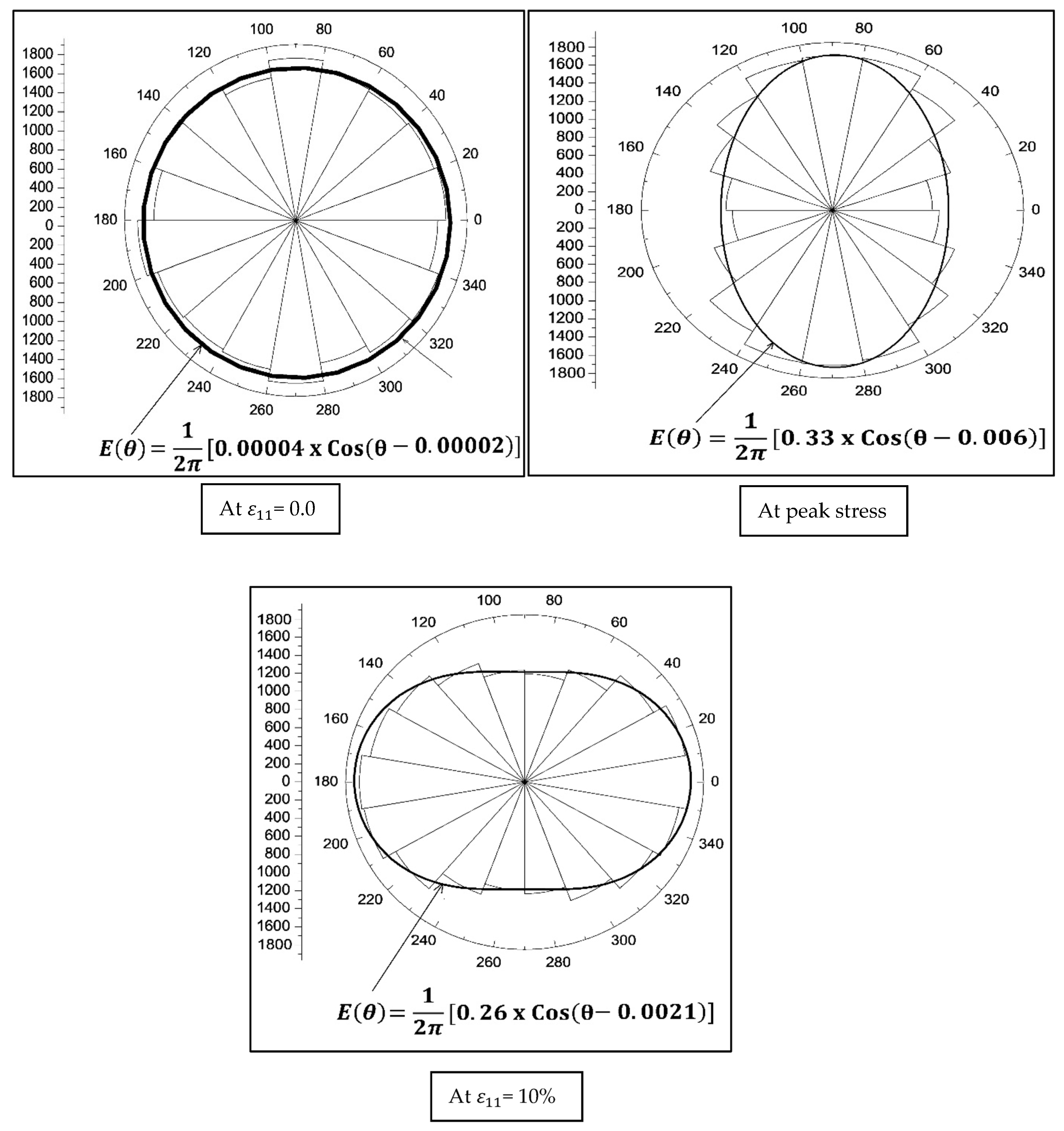
The polar diagram of contact distribution during the shearing for the model with a contact stiffness of 8.45 × 10⁷ (N/m), where = 0.5 and a fixed value of 0.9 is applied to the inter-particle coefficient friction, is presented in Figure 14. Comparing Figure 11 and Figure 14 show that at peak stress, the diameter of the polar diagram in the major direction, representing the number of contacts per segment, reduced from around 3400 to about 3200. This reduction in the number of contacts results in the particulate system becoming less stiff and taking less load. Additionally, the average fabric anisotropy drops from 0.35 to 0.33, indicating the ability of the system with = 0.5 to generate the number of contacts to take more load reduces. The orientation of contacts at the post-peak is also toward the confining stress, with average fabric anisotropy reduced to 0.26.
This reduction in the number of contacts is observed in Figure 15, where the sensitivity of the average coordination number to a reduction in shear contact stiffness from = 1 and = 0.5 for two sets of contact stiffness (i.e., 8.75 × 10⁷ (N/m) and 17 × 107 (N/m)) is compared. At = 0.0, the average coordination number for models with the lower shear contact stiffness value is approximately similar to that obtained from the model with higher shear contact stiffness. From = 0.0 to the axial strain corresponds to the peak stress (see Figure 14), and the average coordination number for all models reduces. However, the models with lower shear contact stiffness experience a higher reduction in average coordination number. At post-peak, the average coordination number significantly decreases for the model with lower shear contact stiffness.
4.4.4. Verification of the Cohesionless Nature of the Synthetic Material Used for Particulate Sand
To verify the cohesionless nature of the synthetic material used for this study, three biaxial tests with different confining pressure values were implemented. Table 12 presents the inter-particle properties along with the size of the sample, initial porosity, PSD, number of particles, and confining pressures used for this study. These samples were isotopically consolidated under different confining pressures before being subjected to shearing under a strain-control approach, as explained in Section 4.4.
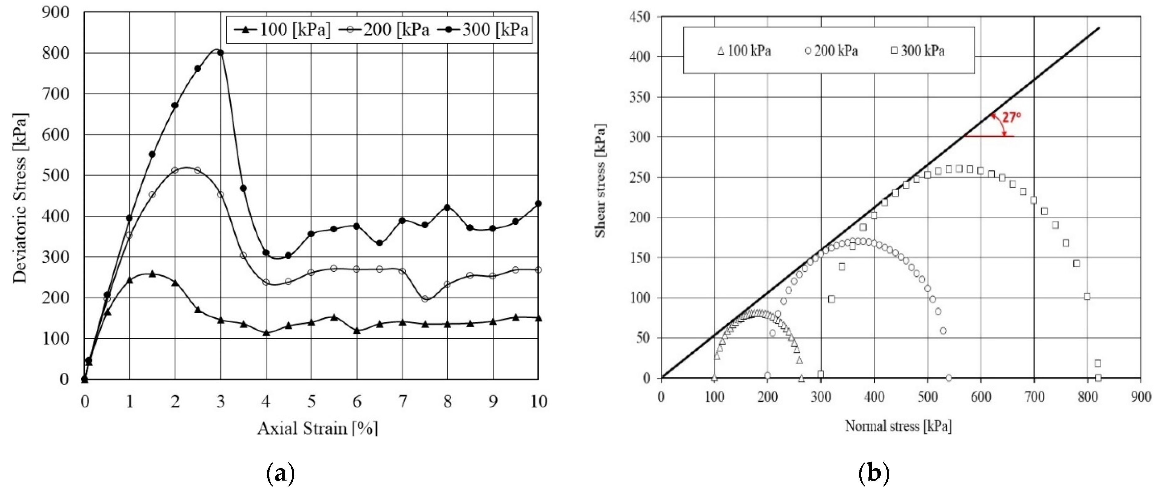
Figure 16a shows the variation of deviatoric stress with axial strain. As expected, an increase in confining pressure leads to an increase in the peak stress. The ratio of peak stress for confining pressure of 300 (kPa) to that of 100 (kPa) is about 3, the ratio of peak stress for confining pressure 300 (kPa) to that of 200 (kPa) is almost 1.5, and the ratio of peak stress for confining pressure of 200 (kPa) to that or 100 (kPa) is approximately 1.0. This shows that these ratios are in good agreement with the ratio 300 (kPa)/100 (kPa), 300 (kPa)/200 (kPa), and 200 (kPa)/100 (kPa), respectively. The Mohr circle of each test, together with the Mohr-Coulomb failure envelope of these three tests, are presented in Figure 16b. The angle of internal friction extracted from the Mohr-Coulomb failure envelope (i.e., 27°) is similar to the angle of internal friction reported in Table 10 for the model using the contact stiffness of 8.45 × 10⁷ (N/m) and the inter-particle coefficient of friction of 0.9. It can be seen that the nature of the synthetic material used for this study is cohesionless.
5. Conclusions
In this paper, thirty-three biaxial DEM tests with rigid walls were implemented to study the critical inter-particle properties and the range over which these properties impact the micro–macro mechanical behaviour. The modelling results show that the elastic parameter, Young’s modulus, with particle diameters varying between 0.5 (mm) and 3.0 (mm), is greatly dependent on the normal contact stiffness, while the angle of friction is strongly dependent on the inter-particle coefficient of friction. It was observed that the inter-particle coefficient of friction between 0.9 and 1.2 produced an angle of internal friction between 27° and 32° such that the relationship between them seems to be linear. These values are compatible with typical ranges of the angle of friction of medium sand. That is, to produce the angle of friction for dense sand, a higher inter-particle coefficient friction (i.e., more than 1.2) should be applied. The angle of internal friction obtained from inter-particle coefficient of friction 0.5 is between 18° and 20°, which is not within the angle of friction of sand. The values of normal contact stiffness between 8.45 × 10⁷ and 17 × 107 with ratios = 1 and = 0.5 results in producing a range of Young’s modulus values of medium sand. However, Young’s modulus produced based on = 0.5 are about 15% less than that estimated from the models applied = 1. The higher normal contact stiffness (e.g., 46 × 107 (N/m) and 150 × 107 (N/m)) produces an unrealistic Young’s modulus for sand. It was observed that Young’s modulus computed from plane stress conditions is about 5% bigger than that calculated from plane strain conditions. Reduction in the value of shear contact stiffness to half of the value of normal contact stiffness led to a decrease in the total number of contacts in load bearing as the particulate system sheared. This indicates the particulate system became less stiff. This change in shear contact stiffness plays a major role in the volumetric behaviour of these systems, including contraction and dilation, meaning Poisson’s ratio is mainly governed by shear contact stiffness. The results show reducing shear contact stiffness resulting in an increase in Poisson’s ratio values for both plane strain and plane stress conditions. The values of Poisson’s ratio for plane strain conditions obtained for those particulate systems applying the normal contact stiffness between 8.45 × 10⁷ and 17 × 107 and = 1 and = 0.5 are within the typical values of Poisson’s ratio of medium sand. That is, to produce Poisson’s ratio values within the typical range of dense sand, the ratio should be less than 0.5. The macro-mechanical behaviour of particulate sand is dictated by inter-particle properties such that a change in one of these parameters results in a significant change in the macro-mechanical behaviour, such as stress–strain and volumetric behaviour. A set of relationships was established between inter-particle properties (including normal contact stiffness and inter-particle coefficient of friction) and macro-machinal parameters such as Young’s modulus, Poisson’s ratio, and angle of internal friction. Reviewing the polar diagram of contact distribution shows that the peak stress and hardening strain behaviour for a particulate system are a function of the number of contacts developed in the major stress direction. The ability of a system to develop the number of contacts is tied to its fabric anisotropy. It was seen that the models use the higher inter-particle coefficient of friction value to develop higher fabric anisotropy and subsequently produce higher peaks and angles of internal friction. This paper only covers three components of ideal disk inter-particle properties, e.g., normal contact stiffness, shear contact stiffness, and particle friction. The impact of other particle-scale parameters, such as particle shape, rolling resistance, and lateral boundary conditions on the macro-mechanical properties, are not covered in this study. This study presents a set of relationships between a wide range of inter-particle properties and elastoplastic parameters for medium and dense sands. These relationships can be used to estimate the inter-particle properties values from lab test data of sands, including elastoplastic parameters for DEM modelling of geotechnical problems. For instance, the first author of this paper applied these relationships to estimate the input data of inter-particle properties of seabed sand from lab test data to simulate the lateral behaviour of the Gravity Base Foundation of an offshore windfarm turbine using PFC2D for an industrial project.
Author Contributions
Conceptualization, A.M.; methodology, A.M.; software, A.M.; validation, A.M.; formal analysis, A.M.; investigation, A.M.; resources, A.M.; data curation, A.M. and K.I.-I.I.E.; writing—original draft preparation, A.M.; writing—review and editing, A.M., Y.S. and K.I.-I.I.E.; visualization, A.M.; supervision, Y.S.; project administration, A.M. All authors have read and agreed to the published version of the manuscript.
Funding
This research received no external funding.
Data Availability Statement
Not applicable.
Conflicts of Interest
The authors declare no conflict of interest.
Nomenclature
| Translational particle velocity | |
| Rotational particle velocity | |
| Stability index of particle | |
| Rotation of | |
| Normal contact deformation | |
| Fabric anisotropy | |
| Time step | |
| Shear contact deformation | |
| θ | Angle of contact force from x-axis and angle friction |
| α | Damping constant |
| Strain rate | |
| Tangential contact stiffness | |
| Normal contact stiffness | |
| Total normal contact force | |
| Total tangential contact force | |
| Particle density | |
| Strain rate | |
| Contact pressure | |
| I | Density scaling factor |
| Confining pressure | |
| Contact force | |
| Inter-particle coefficient of friction particles | |
| F | Resultant force |
| Local damping force | |
| M | Torque |
| Poisson’s ratio | |
| R | Particle radius |
| and | Unite vector |
| t | Deviatoric stress |
| s | Isotropic stress |
| E0 | Initial Young’s modulus |
| Major Strain tensor component in axial direction | |
| Strain tensor component in out-plane lateral direction | |
| Minor Strain tensor component | |
| Volumetric strain | |
| G | Characteristic point |
| Shear strain component in out-off direction | |
| Shear strain component in out-off direction | |
| Major Stress tensor component in axial direction | |
| Stress tensor component in out-plane lateral direction | |
| Minor Stress tensor component | |
| E50 | Secant Young’s modulus at 50% of peak stress |
References
- Antony, S.J. Link between single-particle properties and macroscopic properties in particulate assemblies. Philos. Trans. R. Soc. A Math. Phys. Eng. Sci. 2007, 365, 2879–2891. [Google Scholar] [CrossRef] [PubMed]
- Martin, E.L.; Thornton, C.; Utili, S. Micromechanical investigation of liquefaction of granular media by cyclic 3D DEM tests. Géotechnique 2020, 70, 906–915. [Google Scholar] [CrossRef]
- Wei, J.; Ren, J.; Fu, H. The weakening of inter-particle friction and its effect on mechanical behaviors of granular soils. Comput. Geotech. 2022, 147, 104764. [Google Scholar] [CrossRef]
- Wu, M.; Wang, J.; Wu, F. DEM investigations of failure mode of sands under oedometric loading. Adv. Powder Technol. 2022, 33, 103599. [Google Scholar] [CrossRef]
- Nie, J.Y.; Cao, Z.J.; Li, D.Q.; Cui, Y.F. 3D DEM insights into the effect of particle overall regularity on macro and micro mechanical behaviours of dense sands. Comput. Geotech. 2021, 132, 103965. [Google Scholar] [CrossRef]
- Rothenburg, L.; Bathurst, R.J. Analytical Study of Induced Anisotropy in Idealized Granular Materials. Geotechnique 1989, 39, 601–614. [Google Scholar] [CrossRef]
- Yimsiri, S.; Soga, K. DEM analysis of soil fabric effects on behaviour of sand. Géotechnique 2010, 60, 483–495. [Google Scholar] [CrossRef]
- Momeni, A.; Clarke, B.; Sheng, Y. An Introduction to the Geometrical Stability Index: A Fabric Quantity. Geotechnics 2022, 2, 297–316. [Google Scholar] [CrossRef]
- Robertson, D.; Bolton, M.D. DEM simulations of crushable grains and soils. Powders Grains 2020, 2001, 623–626. [Google Scholar]
- Rothenburg, L.; Nicolaas, P. Kruyt Critical state and evolution of coordination number in simulated granular materials. Int. J. Solids Struct. 2004, 41, 5763–5774. [Google Scholar] [CrossRef]
- Kruyt, N.P.; Rothenburg, L. A strain–displacement–fabric relationship for granular materials. Int. J. Solids Struct. 2019, 165, 14–22. [Google Scholar] [CrossRef]
- Been, K.; Jefferies, G. A state parameter for sands. Géotechnique 1985, 35, 99–112. [Google Scholar] [CrossRef]
- Wood, D.M. Soil Behaviour and Critical State Soil Mechanics; Cambridge University Press: Cambridge, UK, 1990. [Google Scholar]
- Atkinson, J. The Mechanics of Soils and Foundations; CRC Press: Boca Raton, FL, USA, 2017. [Google Scholar]
- Momeni, A. Micro-Mechanical Study of Sand Fabric during Earthquake. Ph. D. Dissertation, University of Leeds, Leeds, UK, 2014. [Google Scholar]
- Reddy, N.S.; He, H.; Senetakis, K. DEM analysis of small and small-to-medium strain shear modulus of sands. Comput. Geotech. 2022, 141, 104518. [Google Scholar] [CrossRef]
- Nardelli, V.; Coop, M.R. The experimental contact behaviour of natural sands: Normal and tangential loading. Géotechnique 2019, 69, 672–686. [Google Scholar] [CrossRef]
- Thornton, C.; Zhang, L. Numerical simulations of the direct shear test. Chem. Eng. Technol. Ind. Chem.-Plant Equip.-Process Eng.-Biotechnol. 2003, 26, 153–156. [Google Scholar] [CrossRef]
- Khosravi, A.; Martinez, A.; DeJong, J.T. Discrete element model (DEM) simulations of cone penetration test (CPT) measurements and soil classification. Can. Geotech. J. 2020, 57, 1369–1387. [Google Scholar] [CrossRef]
- Ciantia, M.O.; Arroyo, M.; O’Sullivan, C.; Gens, A.; Liu, T. Grading evolution and critical state in a discrete numerical model of Fontainebleau sand. Géotechnique 2019, 69, 1–15. [Google Scholar] [CrossRef]
- Gu, X.; Zhang, J.; Huang, X. DEM analysis of monotonic and cyclic behaviors of sand based on critical state soil mechanics framework. Comput. Geotech. 2020, 128, 103787. [Google Scholar] [CrossRef]
- Liu, X.; Zhou, A.; Shen, S.L.; Li, J.; Sheng, D. A micro-mechanical model for unsaturated soils based on DEM. Comput. Methods Appl. Mech. Eng. 2020, 368, 113183. [Google Scholar] [CrossRef]
- Antony, S.J.; Kruyt, N.P. Role of interparticle friction and particle-scale elasticity in the shear-strength mechanism of three-dimensional granular media. Phys. Rev. E 2009, 79, 031308. [Google Scholar] [CrossRef]
- Cavarretta, I.; Coop, M.; O’Sullivan, C. The influence of particle characteristics on the behaviour of coarse grained soils. Géotechnique 2010, 60, 413–423. [Google Scholar] [CrossRef]
- Barreto, D.; O’Sullivan, C. The influence of inter-particle friction and the intermediate stress ratio on soil response under generalised stress conditions. Granul. Matter 2012, 14, 505–521. [Google Scholar] [CrossRef]
- Sandeep, C.S.; Senetakis, K. Effect of Young’s modulus and surface roughness on the inter-particle friction of granular materials. Materials 2018, 11, 217. [Google Scholar] [CrossRef]
- Nie, Z.; Fang, C.; Gong, J.; Liang, Z. DEM study on the effect of roundness on the shear behaviour of granular materials. Comput. Geotech. 2020, 121, 103457. [Google Scholar] [CrossRef]
- Zhao, S.; Evans, T.M.; Zhou, X. Effects of curvature-related DEM contact model on the macro-and micro-mechanical behaviours of granular soils. Géotechnique 2018, 68, 1085–1098. [Google Scholar] [CrossRef]
- Lambe, T.W.; Whitman, R.V. Soil Mechanics; John Wiley & Sons: New York, NY, USA, 1991. [Google Scholar]
- Mahmood, Z.; Iwashita, K. Influence of inherent anisotropy on mechanical behavior of granular materials based on DEM simulations. Int. J. Numer. Anal. Methods Geomech. 2010, 34, 795–819. [Google Scholar] [CrossRef]
- Belheine, N.; Plassiard, J.P.; Donzé, F.V.; Darve, F.; Seridi, A. Numerical simulation of drained triaxial test using 3D discrete element modeling. Comput. Geotech. 2009, 36, 320–331. [Google Scholar] [CrossRef]
- Yang, G.; Yu, T.; Hanlong, L. Numerical simulation of undrained triaxial test using 3D discrete element modeling. Instrum. Test. Model. Soil Rock Behav. 2011, 99–106. [Google Scholar] [CrossRef]
- PFC3D Particle Flow Code in Three Dimensions Manual. Minneapolis, USA. 2011. Available online: https://www.itascacg.com/ (accessed on 1 April 2023).
- Iwashita, K.; Oda, M. Rolling resistance at contacts in simulation of shear band development by DEM. J. Eng. Mech. 1998, 124, 285–292. [Google Scholar] [CrossRef]
- Oda, M.; Iwashita, K. Mechanics of Granular Materials: An Introduction; CRC Press: Boca Raton, FL, USA, 2020. [Google Scholar]
- Sitharam, T.G. Discrete element modelling of cyclic behaviour of granular materials. Geotech. Geol. Eng. 2003, 21, 297–329. [Google Scholar] [CrossRef]
- Cundall, P.A.; Strack, O.D. A discrete numerical model for granular assemblies. Geotechnique 1979, 29, 47–65. [Google Scholar] [CrossRef]
- Itasca Particle Flow Code in Two Dimensions (PFC2D) Manual. Minneapolis, USA. 2014. Available online: https://www.itascacg.com/ (accessed on 1 April 2023).
- O’Sullivan, C.; Bray, J.D.; Riemer, M.F. Influence of particle shape and surface friction variability on response of rod-shaped particulate media. J. Eng. Mech. 2002, 128, 1182–1192. [Google Scholar] [CrossRef]
- German, R.M. Coordination Number Changes During Powder Densification. Powder Technol. 2014, 253, 368–376. [Google Scholar] [CrossRef]
- Ng, T.T. Fabric Evolution of Ellipsoidal Arrays With Different Particle Shapes. J. Eng. Mech. 2001, 127, 994–999. [Google Scholar] [CrossRef]
- Maeda, K. Critical State-based Geo-micromechanics on Granular Flow. AIP Conf. Proc. Am. Inst. Physics. 2009, 1145, 17–24. [Google Scholar]
- Okur, D.V.; Ansal, A. Stiffness degradation of natural fine grained soils during cyclic loading, Soil Dynamics and Earthquake Engineering. Soil Dyn. Earthq. Eng. 2007, 27, 843–854. [Google Scholar] [CrossRef]
- Holtz, R.D.; Kovacs, W.D.; Sheahan, T.C. An Introduction to Geotechnical Engineering; Prentice-Hall: Englewood Cliffs, NJ, USA, 1981; Volume 733. [Google Scholar]
- Head, K.H. Manual of Soil Laboratory Testing; Pentech Press: London, UK, 2006. [Google Scholar]
- Pruiksma, J.P.; Bezuijen, A. Biaxial Test Simulations with PFC2D; Delft University: Mekelweg, The Netherlands, 2002. [Google Scholar]
- Obrzud, R.F. On the use of the Hardening Soil Small Strain model in geotechnical practice. Numer. Geotech. Struct. 2010, 16, 1–17. [Google Scholar]
- Bowles, J.E. Foundation Analysis and Design; McGraw Hill: New York, NY, USA, 1988. [Google Scholar]
- Yamamuro, J.A.; Abrantes, A.E.; Lade, P.V. Effect of strain rate on the stress-strain behavior of sand. J. Geotech. Geoenvironmental Eng. 2011, 137, 1169–1178. [Google Scholar] [CrossRef]
- Chi, L.L.; Qin, J.M.; Chen, X.F. DEM Simulation of Micro-Macro Mechanical Behaviour of Granular Materials. Adv. Mater. Res. 2013, 663, 441–446. [Google Scholar] [CrossRef]
- Coetzee, C.J.; Els, D.N.J. Calibration of granular material parameters for DEM modelling and numerical verification by blade-granular material interaction. J. Terramechanics 2009, 46, 15–26. [Google Scholar] [CrossRef]
Figure 1.
The calculation process in two-dimensional DEM. (a) Initial configuration of the sand assembly. (b) Detecting particles in contact (c) Calculation of inter-particle contact forces (d) Calculation of two in-plane contact forces and moment (e) Calculation of particle movement and rotation (f) Update configuration of the sand assembly.

Figure 2.
The typical behaviour of medium and dense sand (after Momeni [15]).
Figure 2.
The typical behaviour of medium and dense sand (after Momeni [15]).

Figure 3.
The values of inter-particle friction for quartz sand (redrawn after Lambe and Whitman [29]).
Figure 3.
The values of inter-particle friction for quartz sand (redrawn after Lambe and Whitman [29]).

Figure 4.
Particle size distribution used for this study.

Figure 5.
The sensitivity of macro-mechanical behaviour of sand to inter-particle coefficient of frictions: (a) deviatoric stress with axial strain and (b) volumetric strain with axial strain where normal and shear contact stiffness is 8.45 × 10⁷ (N/m).
Figure 5.
The sensitivity of macro-mechanical behaviour of sand to inter-particle coefficient of frictions: (a) deviatoric stress with axial strain and (b) volumetric strain with axial strain where normal and shear contact stiffness is 8.45 × 10⁷ (N/m).

Figure 6.
The sensitivity analysis: (a) inter-particle coefficient of friction vs. peak stress and (b) inter-particle coefficient of friction vs. peak stress.
Figure 6.
The sensitivity analysis: (a) inter-particle coefficient of friction vs. peak stress and (b) inter-particle coefficient of friction vs. peak stress.

Figure 7.
The sensitivity of micro mechanical behaviour of idealised sand to the inter-particle coefficients of friction when normal and shear stiffnesses are constant: (a) Average fabric anisotropy with axial strain (b) average coordination number with axial strain.
Figure 7.
The sensitivity of micro mechanical behaviour of idealised sand to the inter-particle coefficients of friction when normal and shear stiffnesses are constant: (a) Average fabric anisotropy with axial strain (b) average coordination number with axial strain.

Figure 8.
The sensitivity of deviatoric stress, volumetric strain, and peak stress to the normal contact stiffness. (a) Macro-mechanical responses to various µ when kn = ks = 8.45 × 10⁷ (N/m). (b) Macro-mechanical responses to various µ when kn = ks =17 × 107 (N/m). (c) Macro-mechanical responses to various µ when kn = ks = 46 × 107 (N/m). (d) Macro-mechanical responses to various µ when kn = ks =133 × 107 (N/m). (e) Macro-mechanical responses to various µ when kn = ks = 150 × 107 (N/m). (f) The variation of peak stress to various µ and kn where kn/ks = 1.

Figure 9.
The sensitivity of E50 to the various particle normal contact stiffnesses: (a) plane strain and (b) plane stress.
Figure 9.
The sensitivity of E50 to the various particle normal contact stiffnesses: (a) plane strain and (b) plane stress.

Figure 10.
The sensitivity of Poisson’s ratio to the various particle normal stiffness: (a) plane strain and (b) plane stress.
Figure 10.
The sensitivity of Poisson’s ratio to the various particle normal stiffness: (a) plane strain and (b) plane stress.

Figure 11.
The evolution of contact distribution of particulate sand kn = ks = 8.45 × 10⁷ (N/m) where = 1, and inter-particle coefficient of friction is 0.9.
Figure 11.
The evolution of contact distribution of particulate sand kn = ks = 8.45 × 10⁷ (N/m) where = 1, and inter-particle coefficient of friction is 0.9.

Figure 12.
The sensitivity of sand to the different contact stiffness when inter-particle coefficient of friction is 0.9: (a) average fabric anisotropy vs. axial strain and (b) average coordination number vs. axial strain.
Figure 12.
The sensitivity of sand to the different contact stiffness when inter-particle coefficient of friction is 0.9: (a) average fabric anisotropy vs. axial strain and (b) average coordination number vs. axial strain.

Figure 13.
Deviatoric stress with axial strain and volumetric strain with axial strain. (a) Macro-mechanical responses to = 1.0 and = 0.5 when kn = 8.45 × 10⁷ (N/m) at the fixed µ = 0.9. (b) Macro-mechanical responses to = 1.0 and = 0.5 when kn = 17 × 107 (N/m) at the fixed µ = 0.9. (c) Macro-mechanical responses to = 1.0 and = 0.5 when kn = 46 × 107 (N/m) at the fixed µ = 0.9. (d) Macro-mechanical responses to = 1.0 and = 0.5 when kn = 133 × 107 (N/m) at the fixed µ = 0.9. (e) Macro-mechanical responses to = 1.0 and = 0.5 when kn = 150 × 107 (N/m) at the fixed µ = 0.9.

Figure 14.
The evolution of contact distribution of particulate sand kn = ks = 8.45 × 10⁷, where = 0.5 and inter-particle coefficient of friction is 0.9.
Figure 14.
The evolution of contact distribution of particulate sand kn = ks = 8.45 × 10⁷, where = 0.5 and inter-particle coefficient of friction is 0.9.

Figure 15.
The sensitivity of average coordination number of sand to the various particle shear stiffness.
Figure 15.
The sensitivity of average coordination number of sand to the various particle shear stiffness.

Figure 16.
(a) Deviatoric stress with axial strain for three different isotropic stress and (b) Mohr-Coulomb failure envelope.
Figure 16.
(a) Deviatoric stress with axial strain for three different isotropic stress and (b) Mohr-Coulomb failure envelope.


Table 1.
Advantages and limitations in the use of 2D and 3D modelling.
| Two-Dimensional DEM Model | Three-Dimensional DEM Model | ||
|---|---|---|---|
| Advantages | Limitations | Advantages | Limitations |
| Less number of particles are required to be generated to study a problem | Three degrees of freedom are used in the calculation cycles (two in-plane displacements and one in-plane moment) | Six degrees of freedom are used in the calculation cycles | Greater numbers of particles are required to be generated to study a problem |
| Cost of calculations is relatively less | The impact of out-of-plane forces and moments are not considered in the macro–micro responses | The impact of out-of-plane forces and moments are considered on the macro–micro responses | The cost of calculations is relatively high. Since DEM tracks each individual particle and its interactions over time, an increase in the number of particles increases the computational time |
| Suitable for 2D plane strain and plane stress problems | The out-of-plane forces, which are essential to enforcing a state of the plane strain and plane stress, are not present. | Produces more realistic macro–micro responses | The application of 3D DEM to produce the deformable boundary conditions is complicated |
| Fewer cycles are required for particulate systems to reach equilibrium | The application of 2D DEM to produce the deformable boundary conditions is complicated | More cycles are required for particulate systems to reach equilibrium | |
| Enabling clear visualisation as particle motion is restricted to one plane | Less clear visualisation as particle motion is restricted to one plane | ||
| More cost-effective for the models subjected to dynamic loading due to computational capabilities | Less cost-effective for the models subjected to dynamic loading due to limited computational capabilities | ||
Table 2.
The micro-mechanical parameters used for the sensitivity analysis (after Momeni [15]).
Table 2.
The micro-mechanical parameters used for the sensitivity analysis (after Momeni [15]).
| (N/m) | = 1 | = 0.5 | Inter-Particle Coefficient of Friction |
|---|---|---|---|
| (N/m) | (N/m) | ||
| 8.45 × 10⁷ | 8.45 × 10⁷ | 4.22 × 10⁷ | 0.5, 0.9, 1.2 |
| 17 × 107 | 17 × 107 | 8.50 × 10⁷ | 0.5, 0.9, 1.2 |
| 46 × 107 | 46 × 107 | 23 × 107 | 0.5, 0.9, 1.2 |
| 133 × 107 | 133 × 107 | 66.5 × 10⁷ | 0.5, 0.9, 1.2 |
| 150 × 107 | 150 × 107 | 75 × 107 | 0.5, 0.9, 1.2 |
Table 3.
The input data for this study.
| Porosity after radius enlargement | 0.12 |
| Range of Particle Size Distribution PSD (mm) | 0.5–3 (refer to Figure 4) |
| (N/m) (Normal contact stiffness) | Refer to Table 2 |
| (N/m) (Shear contact stiffness) | Refer to Table 2 |
| μ (Inter-particle coefficient of friction) | Refer to Table 2 |
| α (Damping constant) | 0.8 |
| Coefficient friction of particle-platen | 0.0 |
| Width (mm) | 75 |
| Height (mm) | 150 |
| 2650 |
Table 4.
Typical bulk properties of sand.
| Strength Parameters | Medium Sand | Dense Sand |
|---|---|---|
| (MPa) | 30~50 [47] 25~50 [48] | 50~80 [47] 50~81 [48] |
| 0.2~0.35 [48] | 0.3~0.4 [48] | |
| Friction angle (°) | 30~36 [47] | 36~41 [47] |
Table 5.
The input data for sensitivity of sand system to the inter-particle coefficient of friction.
Table 5.
The input data for sensitivity of sand system to the inter-particle coefficient of friction.
| kn = ks (N/m) | Inter-Particle Coefficient of Friction |
|---|---|
| 8.45 × 10⁷ | 0.5, 0.9, 1.2 |
| 17 × 107 | 0.5, 0.9, 1.2 |
| 46 × 107 | 0.5, 0.9, 1.2 |
| 133 × 107 | 0.5, 0.9, 1.2 |
| 150 × 107 | 0.5, 0.9, 1.2 |
Table 6.
The sensitivity analysis: inter-particle coefficient friction vs. E50 for plane strain and plane stress.
Table 6.
The sensitivity analysis: inter-particle coefficient friction vs. E50 for plane strain and plane stress.
| Contact Stiffness (N/m) | Inter-Particle Coefficient of Friction | |||
|---|---|---|---|---|
| 0.5 | 0.9 | 1.2 | ||
| kn = ks = 8.45 × 10⁷ | E50 (plane strain) (MPa) | 32 | 35 | 35 |
| E50 (plane stress) (MPa) | 34 | 36 | 36 | |
| kn = ks = 17 × 107 | E50 (plane strain) (MPa) | 61 | 67 | 68 |
| E50 (plane stress) (MPa) | 64 | 70 | 71 | |
| kn = ks = 46 × 107 | E50 (plane strain) (MPa) | 162 | 173 | 180 |
| E50 (plane stress) (MPa) | 170 | 181 | 186 | |
| kn = ks = 133 × 107 | E50 (plane strain) (MPa) | 388 | 444 | 478 |
| E50 (plane stress) (MPa) | 417 | 470 | 500 | |
| kn = ks = 150 × 107 | E50 (plane strain) (MPa) | 463 | 535 | 540 |
| E50 (plane stress) (MPa) | 494 | 563 | 570 | |
Table 7.
The sensitivity analysis: inter-particle coefficient friction vs. Poisson’s ratio for plane strain and plane stress.
Table 7.
The sensitivity analysis: inter-particle coefficient friction vs. Poisson’s ratio for plane strain and plane stress.
| Contact Stiffness (N/m) | Inter-Particle Coefficient of Friction | |||
|---|---|---|---|---|
| 0.5 | 0.9 | 1.2 | ||
| kn = ks = 8.45 × 10⁷ | v (plane strain) | 0.17 | 0.18 | 0.21 |
| v (plane stress) | 0.20 | 0.22 | 0.27 | |
| kn = ks = 17 × 107 | v (plane strain) | 0.18 | 0.19 | 0.22 |
| v (plane stress) | 0.22 | 0.23 | 0.28 | |
| kn = ks = 46 × 107 | v (plane strain) | 0.19 | 0.2 | 0.24 |
| v (plane stress) | 0.23 | 0.25 | 0.32 | |
| kn = ks = 133 × 107 | v (plane strain) | 0.21 | 0.23 | 0.25 |
| v (plane stress) | 0.27 | 0.30 | 0.33 | |
| kn = ks = 150 × 107 | v (plane strain) | 0.21 | 0.25 | 0.27 |
| v (plane stress) | 0.27 | 0.33 | 0.37 | |
Table 8.
The inter-particle parameters for additional fifteen biaxial tests to investigate the sensitivity of system to the shear contact stiffness.
Table 8.
The inter-particle parameters for additional fifteen biaxial tests to investigate the sensitivity of system to the shear contact stiffness.
| (N/m) | = 0.5 | Inter-Particle Coefficient of Friction |
|---|---|---|
| (N/m) | ||
| 8.45 × 10⁷ | 4.22 × 10⁷ | 0.5, 0.9, 1.2 |
| 17 × 107 | 8.55 × 10⁷ | 0.5, 0.9, 1.2 |
| 46 × 107 | 23.0 × 10⁷ | 0.5, 0.9, 1.2 |
| 133 × 107 | 66.5 × 10⁷ | 0.5, 0.9, 1.2 |
| 150 × 107 | 75.0 × 10⁷ | 0.5, 0.9, 1.2 |
Table 9.
The sensitivity of E50 for both plane strain and plane stress to the various particle shear stiffness.
Table 9.
The sensitivity of E50 for both plane strain and plane stress to the various particle shear stiffness.
| Contact Stiffness (N/m) | Inter-Particle Coefficient of Friction | |||
|---|---|---|---|---|
| 0.5 | 0.9 | 1.2 | ||
| = 0.5: kn = 8.45 × 10⁷ | E50 (plane strain) (MPa) | 27 | 28 | 29 |
| E50 (plane stress) (MPa) | 29 | 30 | 31 | |
| = 0.5: kn = 17 × 107 | E50 (plane strain) (MPa) | 56 | 59 | 60 |
| E50 (plane stress) (MPa) | 60 | 61 | 63 | |
| = 0.5: kn = 46 × 107 | E50 (plane strain) (MPa) | 128 | 141 | 143 |
| E50 (plane stress) (MPa) | 140 | 151 | 153 | |
| = 0.5: kn = 133 × 107 | E50 (plane strain) (MPa) | 353 | 416 | 417 |
| E50 (plane stress) (MPa) | 380 | 445 | 450 | |
| = 0.5: kn = 150 × 107 | E50 (plane strain) (MPa) | 380 | 445 | 447 |
| E50 (plane stress) (MPa) | 420 | 480 | 480 | |
Table 10.
The sensitivity of Poisson’s ratio to the various particle shear stiffness.
| Contact Stiffness (N/m) | Inter-Particle Coefficient of Friction | |||
|---|---|---|---|---|
| 0.5 | 0.9 | 1.2 | ||
| = 0.5: kn = 8.45 × 10⁷ | v (plane strain) | 0.22 | 0.23 | 0.24 |
| v (plane stress) | 0.28 | 0.30 | 0.32 | |
| = 0.5: kn = 17 × 107 | v (plane strain) | 0.23 | 0.24 | 0.25 |
| v (plane stress) | 0.30 | 0.32 | 0.33 | |
| = 0.5: kn = 46 × 107 | v (plane strain) | 0.25 | 0.25 | 0.26 |
| v (plane stress) | 0.33 | 0.33 | 0.35 | |
| = 0.5: kn = 133 × 107 | v (plane strain) | 0.26 | 0.27 | 0.27 |
| v (plane stress) | 0.35 | 0.37 | 0.37 | |
| = 0.5: kn = 150 × 107 | v (plane strain) | 0.27 | 0.28 | 0.29 |
| v (plane stress) | 0.37 | 0.39 | 0.41 | |
Table 11.
The sensitivity of angle of friction to the various particle shear stiffness.
| Normal Contact Stiffness (N/m) | Inter-Particle Coefficient of Friction | ||||
|---|---|---|---|---|---|
| 0.5 | 0.9 | 1.2 | |||
| 8.45 × 10⁷ | = 1.0 | Angle of internal friction | 19 | 27 | 30 |
| = 0.5 | Angle of internal friction | 18 | 26 | 28 | |
| 17 × 107 | = 1.0 | Angle of internal friction | 20 | 27 | 30 |
| = 0.5 | Angle of internal friction | 18 | 26 | 28 | |
| 46 × 107 | = 1.0 | Angle of internal friction | 20 | 27 | 30 |
| = 0.5 | Angle of internal friction | 18 | 26 | 28 | |
| 133 × 107 | = 1.0 | Angle of internal friction | 20 | 27 | 30 |
| = 0.5 | Angle of internal friction | 20 | 26 | 29 | |
| 150 × 107 | = 1.0 | Angle of internal friction | 20 | 28 | 32 |
| = 0.5 | Angle of internal friction | 20 | 27 | 31 | |
Table 12.
The input properties used for sensitivity analysis of sand to the different confining pressures.
Table 12.
The input properties used for sensitivity analysis of sand to the different confining pressures.
| Test No. | (N/m) | (N/m) | Width (cm) | Height (cm) | Range of PSD (mm) | Confining Pressure (kPa) | ||
|---|---|---|---|---|---|---|---|---|
| 1 | 8.45 × 10⁷ | 8.45 × 10⁷ | 0.9 | 7.5 | 15.0 | 0.12 | 0.5–3 | 100 |
| 2 | 8.45 × 10⁷ | 8.45 × 10⁷ | 0.9 | 7.5 | 15.0 | 0.12 | 0.5–3 | 200 |
| 3 | 8.45 × 10⁷ | 8.45 × 10⁷ | 0.9 | 7.5 | 15.0 | 0.12 | 0.5–3 | 300 |
Disclaimer/Publisher’s Note: The statements, opinions and data contained in all publications are solely those of the individual author(s) and contributor(s) and not of MDPI and/or the editor(s). MDPI and/or the editor(s) disclaim responsibility for any injury to people or property resulting from any ideas, methods, instructions or products referred to in the content. |
© 2023 by the authors. Licensee MDPI, Basel, Switzerland. This article is an open access article distributed under the terms and conditions of the Creative Commons Attribution (CC BY) license (https://creativecommons.org/licenses/by/4.0/).
Share and Cite
MDPI and ACS Style
Momeni, A.; Eshiet, K.I.-I.I.; Sheng, Y. The Sensitivity of Micro—Macro Mechanical Behaviour of Sand to the Inter-Particle Properties. Geotechnics 2023, 3, 416-445. https://doi.org/10.3390/geotechnics3020024
AMA Style
Momeni A, Eshiet KI-II, Sheng Y. The Sensitivity of Micro—Macro Mechanical Behaviour of Sand to the Inter-Particle Properties. Geotechnics. 2023; 3(2):416-445. https://doi.org/10.3390/geotechnics3020024
Chicago/Turabian StyleMomeni, Ali, Kenneth Imo-Imo Israel Eshiet, and Yong Sheng. 2023. "The Sensitivity of Micro—Macro Mechanical Behaviour of Sand to the Inter-Particle Properties" Geotechnics 3, no. 2: 416-445. https://doi.org/10.3390/geotechnics3020024