Review of Applicable Outlier Detection Methods to Treat Geomechanical Data

Abstract

The reliability of geomechanical models and engineering designs depend heavily on high-quality data. In geomechanical projects, collecting and analyzing laboratory data is crucial in characterizing the mechanical properties of soils and rocks. However, insufficient lab data or underestimating data treatment can lead to unreliable data being used in the design stage, causing safety hazards, delays, or failures. Hence, detecting outliers or extreme values is significant for ensuring accurate geomechanical analysis. This study reviews and categorizes applicable outlier detection methods for geomechanical data into fence labeling methods and statistical tests. Using real geomechanical data, the applicability of these methods was examined based on four elements: data distribution, sensitivity to extreme values, sample size, and data skewness. The results indicated that statistical tests were less effective than fence labeling methods in detecting outliers in geomechanical data due to limitations in handling skewed data and small sample sizes. Thus, the best outlier detection method should consider this matter. Fence labeling methods, specifically, the medcouple boxplot and semi-interquartile range rule, were identified as the most accurate outlier detection methods for geomechanical data but may necessitate more advanced statistical techniques. Moreover, Tukey’s boxplot was found unsuitable for geomechanical data due to negative confidence intervals that conflicted with geomechanical principles.

1. Introduction

The process of data analysis is a crucial step in experimental studies because the results significantly influence engineering decisions. In geotechnical engineering, natural materials such as soil or rock exhibit inherent variability, which can lead to significant uncertainties in data analysis. These natural uncertainties arise from the formation process and alterations over time, with the primary source varying depending on the type of geomechanical parameter being measured [1,2]. For example, intact rock strength can be affected by variations in petrographic characteristics, such as mineral composition, texture, microstructures, and degree of chemical alteration. Meanwhile, deformability parameters such as Young’s modulus can be affected by water content, degree of jointing, and blasting near mining areas [3]. The variation in laboratory data must also be statistically examined to exclude any possible abnormalities. As a result, even when the samples are properly prepared and the testing protocols strictly followed, their test findings are undoubtedly dispersed, and they should be taken as raw data with certain abnormal datapoints that distort the geomechanical analysis conclusions. Some laboratory measurements appear to be significantly outside of the expected range. These extreme values are known as outliers and can have a detrimental impact on data analysis [4,5,6]. An appropriate procedure must be applied to address the cause of this anomaly [7]. According to Peirce [8], outliers are observations in a dataset that show patterns differing from the bulk of observations in the sample and can significantly violate the distribution assumptions, such as analysis of variance (ANOVA) and regression. Hence, before any decisions are made, the outliers should be detected and dealt with in the dataset, because doing so results in a better fit for parametric statistical models.

The methods of identifying outliers in engineering are mostly case specific and depend on the conditions and objectives of the analysis. In fact, the selection of the most appropriate methods for detecting outliers is crucial and requires the engineering judgment to be considered because the identified outliers should also be reasonable from the viewpoint of geomechanics. Some well-known approaches for outlier detection in the literature are frequently utilized. Peirce [8] was the first to develop a criterion for identifying the outliers in a dataset, based on regression analysis, but this test is less well known than other methods [8]. The most widely used outlier method is boxplots, which has been applied in numerous fields of study. The boxplot has gained popularity in analyzing geomechanical data due to its simplicity and visual appeal. This technique has been utilized in a range of applications such as assessing the variability of rock strength and deformability parameters, as demonstrated by Tiryaki [9], Heidarzadeh et al. [10], Shirani Faradonbeh et al. [11], and Bozorgzadeh et al. [12], and also in several rockburst analyses conducted by Xue et al. [13], Roy et al. [14], and Zhang et al. [15]. Additionally, some researchers utilized boxplots to find the outlier of machine learning analysis conducted to study slope stability [16,17,18]. Boxplots have some limitations, such as their inapplicability in greatly skewed data, which was later improved. Even though modifications have been made to address this limitation, no known geomechanical studies have utilized the modified boxplot to identify outliers. Another useful outlier detection method is Grubbs’ test, which is commonly used in various engineering fields, particularly in quality control and industrial engineering [19]. In civil engineering, Grubbs’ test was used to identify outliers in geotechnical data, such as soil properties, rock mechanics, and foundation performance [20,21]. Several studies applied Grubbs’ test to find the possible outliers in the shear strength data of rock at the 5% confidence level [22,23]. Grubbs’ test assumes that the data are normally distributed, which is why it may not be appropriate for datasets that are not normally distributed. Apart from these methods, which were mostly applied on lab data, Chauvenet’s test was used to find the irregular data of the Schmidt hammer test, which was confirmed by the International Society of Rock Mechanics [24,25,26,27]. Dixon’s test is another method that can be used to identify outliers and has been rarely utilized in geomechanics [28]. Overall, employing these methods helps engineers eliminate datapoints that are not representative of the underlying population and may skew the results of their analyses, thus improving the accuracy and reliability of the results.

The choice of an appropriate outlier detection method depends on the type and distribution of the data being analyzed and the objectives of the analysis. Some methods may be better suited for certain types of data, while others may be more appropriate for specific distributions. In general, a combination of methods should be used to detect outliers in geomechanical investigations because each method has its own strengths and limitations. Geomechanical data tend to be skewed because of a range of potential biases, including observer bias, instrument error, sampling bias, and inaccuracies in data interpretation. For this purpose, robust methods such as boxplots may be a proper choice because they are not sensitive to the shape of the data distribution and extreme values. However, some important tasks include the careful consideration of the assumptions and limitations of each method and the validation of the results by using multiple methods, especially when the dataset is small or when outliers have important implications.

The objective of this study is to improve the understanding of outlier detection methods in the geomechanical field by addressing two important goals. Firstly, we conduct a comprehensive overview of different outlier detection methods and evaluate their advantages and drawbacks in geomechanical domain; secondly, we determine the applicability of certain appropriate methods on real geomechanical data. For this purpose, an innovative methodology is developed to compare the applied methods. To further guide practitioners, some informative figures and flowcharts were created to provide a better understanding of the outlier detection process.

This study involved the collection and classification of all available outlier identification techniques in the literature. The methods were categorized based on their ability to analyze different types of data and the statistical assumptions used in each method. It aimed to provide a clear explanation of the mathematical formulation of each method and then select the most appropriate outlier detection methods for the geomechanical data by assessing their suitability using specific statistical principles, which had not been applied in previous studies. This approach would help engineers select the best detection technique for their specific needs. Through a critical analysis of existing literature and a comparison of the performance of different methods, this paper will provide valuable insights into the context of outlier detection and foster the development of more effective strategies for detecting outliers in engineering applications.

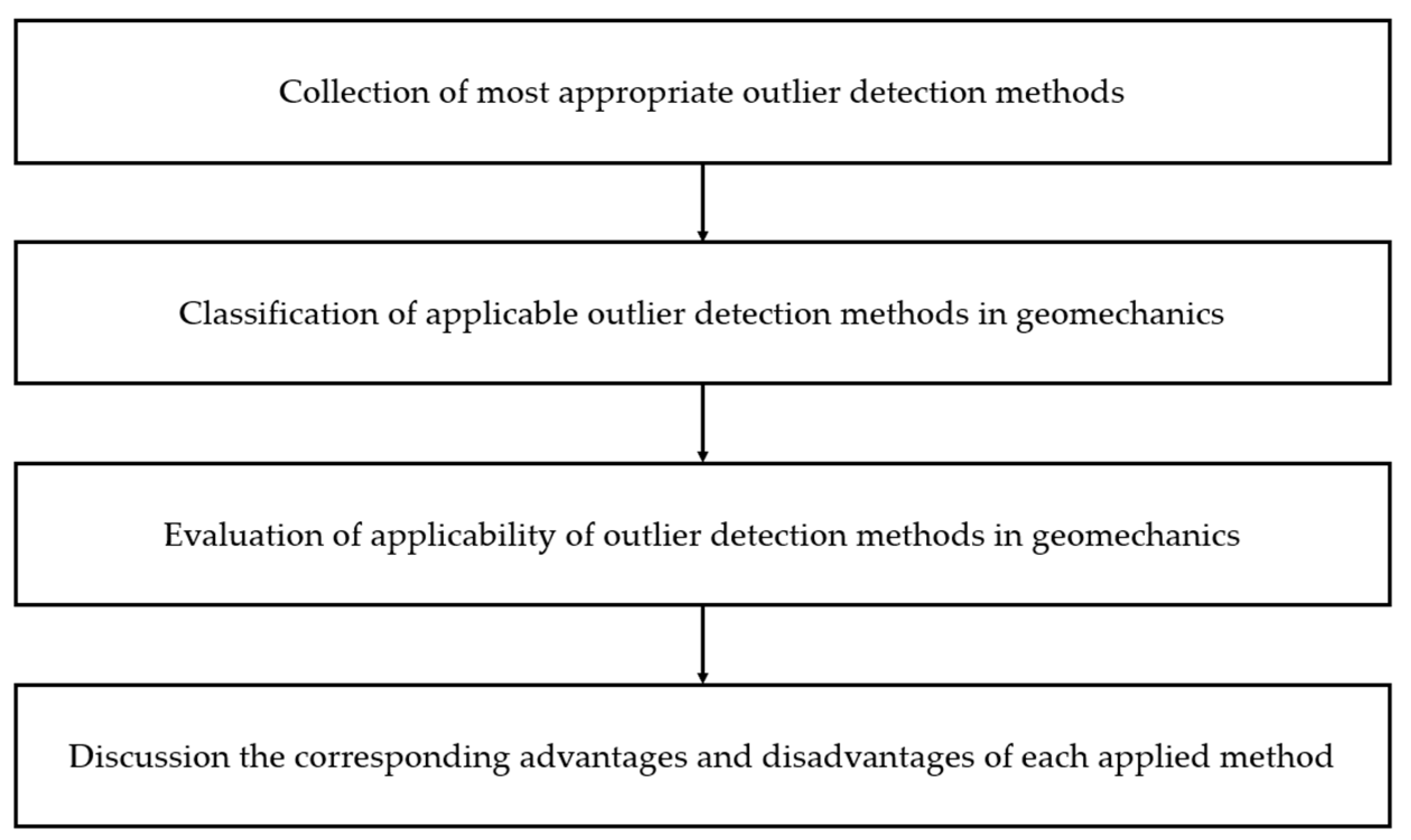
2. Methodology

An appropriate methodology is developed to classify outlier detection methods such that their suitability in geomechanics is examined to help engineers obtain more accurate and reliable results. This methodology comprises four steps (Figure 1). First, a thorough review of various outlier detection techniques, including traditional statistical methods and more recent techniques, is conducted. Collecting and reviewing different methods can establish a comprehensive understanding of various techniques and their capabilities. 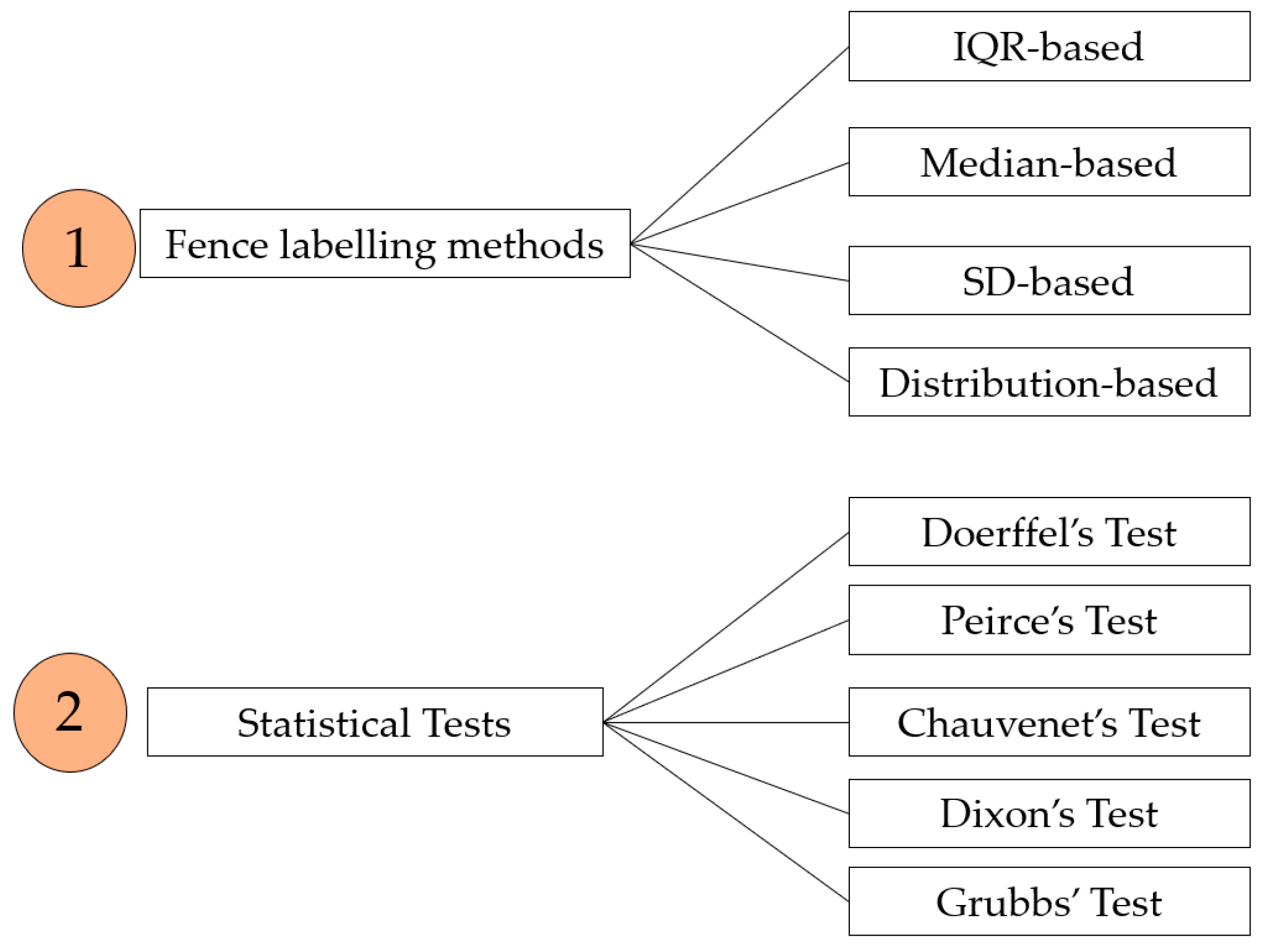Second, the applicable outlier detection techniques for the field of geomechanics are classified. This step is crucial because geomechanical data can vary significantly in terms of their distribution, size, and complexity. Therefore, the choice of outlier detection technique should be based on factors such as the nature of the data and the computational requirements of each method. Third, the applicability of each method is evaluated based on its practical consideration (i.e., robustness and ease of implementation). The assessment procedure considers four elements: the capability of the methods to handle non-normal distributions of data, their responsiveness toward extreme values, their appropriateness for managing large datasets, and their recognition of skewness in the data. Finally, the strengths and weaknesses of each method are discussed by highlighting their pros and cons, thus providing a proper framework for informed decision-making in the field of geomechanics.

3. Classification of Outlier Detection Methods in Geomechanics

We conducted a comprehensive literature review to gather information about existing methods proposed for identifying outliers. Each outlier test and its application domains were studied in detail, which includes understanding the mathematical formulation of the method, the assumptions made, and the types of data that each method is designed to work with, as well as the specific requirements of the problem that the method is designed to solve.

In statistics, outliers are typically detected using both univariate and multivariate methods. Univariate methods are designed to identify outliers in a single-variable dataset, while multivariate methods can detect outliers in multiple variables simultaneously, where outliers in one variable may impact other variables. Multivariate data often have a problem of swamping, which means that the presence of an outlier in one variable can swamp the presence of an outlier in another variable.

In geomechanical studies, the data can be taken as univariate because of their practicality and ease of implementation. In fact, these data include mechanical properties of rocks, such as rock strength or deformability values, in which the outliers are usually identified based on several statistical measures such as mean, standard deviation, and percentiles. In this study, we classify the outlier methods in geomechanics into two groups: fence labeling methods and statistical tests (illustrated in Figure 2).

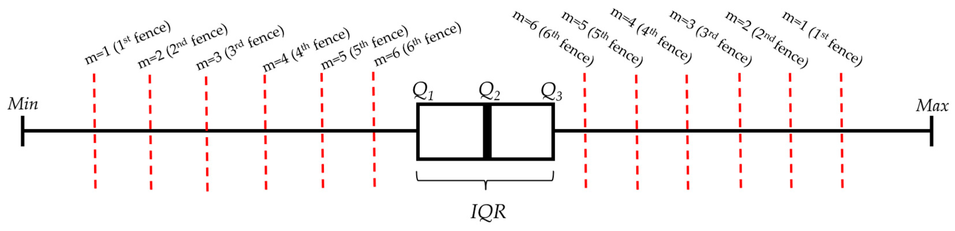
3.1. Fence Labeling Methods

In the fence labeling approach, two fences should be created in the lower and upper thresholds of the dataset as a first step in identifying the possible outliers. Then, a range of observations is distinguished from the rest of the data such that the datapoints outside this range are considered outliers. This range can be specified through several approaches, classified in four groups: interquartile range (IQR)-, median-, SD-, and distribution-based methods [4,29].

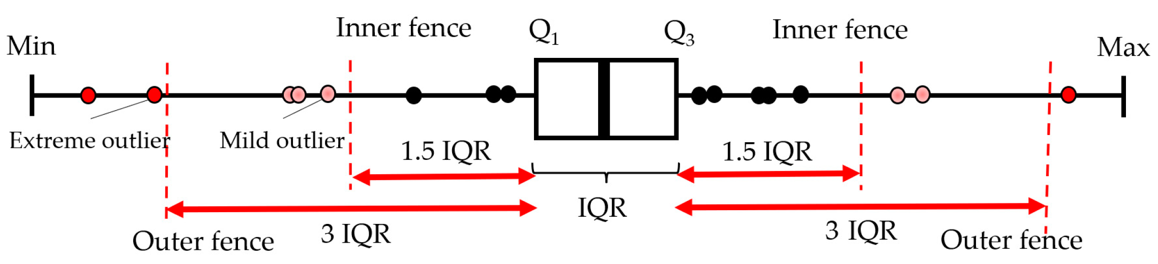
3.1.1. IQR-Based Methods

The box and whisker plot (often known as boxplot), introduced by Tukey [30], is an outlier detection method based on IQR. The boxplot is popular among researchers in various engineering fields because of its relative efficacy, simplicity, and ease of interpretation [31,32,33,34]. It is a data visualization technique for quickly displaying data dispersion and identifying the outliers by means of two fences in the lower and upper bounds. This method utilizes robust statistical tools such as the IQR and the first (Q₁) and third (Q₃) quartiles. These tools are designed to be less sensitive to extreme values in data. If data are sorted in ascending order, then Q₁ represents the value below which 25% of the datapoints lie, while Q₃ is the value below which 75% of the observations are situated, and IQR is the difference between Q₁ and Q₃ (see Figure 3). Outliers are detected by building the upper and lower fences using Equation (1), beyond which the values are considered as outliers.

Tukey proposed k = 1.5 to identify mild outliers between the inner and outer fences and k = 3.0 to label extreme outliers beyond the outer fences. Hoaglin and Iglewicz [35] stated that using k = 1.5 may detect extra outliers [36]. Gignac [37] suggested k = 2.2 for sample sizes between 20 and 300.

Table 1. Summary of suggested IQR-based methods along with corresponding formulas ($f_L$ and $f_U$ are fences in the lower and upper thresholds, respectively).

Author (Year)	Method	Formula	Equation
Tukey (1977) [30]	Traditional boxplot	$\{\begin{array}{c}{f}_L=Q_1-k\times IQR \\ f_U=Q_3+k\times IQR\end{array}$	(1)
Barbato et al. (2011) [4]	Log boxplot	$\{\begin{array}{c}{f}_L=Q_1-1.5\times IQR\left[1+0.1\log \left(n/10\right)\right] \\ f_U=Q_3-1.5\times IQR\left[1+0.1\log \left(n/10\right)\right]\end{array}$	(2)
Schwertman and de Silva (2007) [38]	Sequential fences	$\{\begin{array}{c}{f}_L=Q_2-\frac{t_{df,{\alpha }_{nm}}}{k_n}\left(IQR\right) \\ f_U=Q_2+\frac{t_{df,{\alpha }_{nm}}}{k_n}\left(IQR\right)\end{array}$	(3)
		$d_f=7.6809524+0.5294156n-0.00237n^2$	(4)
Carling (2000) [39]	Median rule	$\{\begin{array}{c}{f}_L=Q_2-2.3 \left(IQR\right) \\ f_U=Q_2+2.3 \left(IQR\right)\end{array}$	(5)
Kimber (1990) [40]	SIQR rule	$\{\begin{array}{c}{f}_L=Q_1-1.5 \left[2\times SIQ{R}_L\right] \\ f_U=Q_3+1.5 \left[2\times SIQ{R}_U\right]\end{array}$	(6)
		$\{\begin{array}{c}SIQ{R}_L=\left(Q_2-Q_1\right)\\ SIQ{R}_U=\left(Q_3-Q_2\right)\end{array}$	(7)
Walker et al. (2018) [31]	Mix of SIQR and IQR	$\{\begin{array}{c}{f}_L=Q_1-1.5 \left[IQR\times \frac{1-B_c}{1+B_c}\right] \\ f_U=Q_3+1.5 \left[IQR\times \frac{1+B_c}{1-B_c}\right]\end{array}$	(8)
		$B_c=\frac{SIQ{R}_U-SIQ{R}_L}{SIQ{R}_U+SIQ{R}_L}$	(9)
Hubert and Vandervieren (2008) [41]	MC boxplot	$ifMC>0\to \{\begin{array}{c}{f}_L=Q_1-1.5e^{-4MC}IQR\\ f_U=Q_3+1.5e^{+3MC}IQR\end{array}$	(10)
		$ifMC<0\to \{\begin{array}{c}{f}_L=Q_1-1.5e^{-3MC}IQR\\ f_U=Q_3+1.5e^{+4MC}IQR\end{array}$	(11)
		$\{\begin{array}{c}MC=\begin{array}{c}median\\ x_i\le Q_2\le x_j\end{array}h \left(x_i,x_j\right)\\ h \left(x_i,x_j\right)=\frac{\left(x_j-Q_2\right)-\left(Q_2-x_i\right)}{x_j-x_i}\end{array}$	(12)

represents proposed formulas for IQR-based methods, such as Tukey’s boxplot, and related techniques. Their timeline-based summary is briefly presented in Figure 4.

Tukey’s boxplot did not consider the effect of sample size on fences, although it has a crucial effect, particularly in small sample sizes. Barbato et al. [4] added the sample size (n) in a logarithmic relationship (Equation (2)). In this modified boxplot, the data should follow a normal distribution.

Schwertman and de Silva [38] proposed a more advanced approach called sequential fences, which divides the dataset into subgroups to consider the effect of sample size. Each subgroup has its own fences (Figure 5). The method creates a sequence of fences in the data, where the first fence (m = 1) is checked for minimum and maximum values, and if labeled as an outlier, then the second fence (m = 2) is focused on the second most extreme values. This process can proceed up to six fences [38]. However, the sequential fences are valid only for a sample size between 20 and 100. In this method, the second quartile (Q₂) is utilized in creating fences, presented in Equations (3) and (4) (to calculate ${\alpha }_{nm}$ and $k_n$ in Equation (3); see Schwertman and de Silva [38]). Even though it can identify outliers very accurately, the sequential fences method remains relatively obscure in the civil engineering literature.

Carling [39] modified Tukey’s boxplot by replacing the median with quartiles to improve its accuracy for skewed data (see Equation (5)), but it has not gained as much popularity as the original boxplot. In skewed data, applying Tukey’s boxplot may label some normal datapoints as outliers and violate the assumption of a symmetric or nearly symmetric distribution. Several studies have attempted to adjust the boxplot to be applicable for skewed datasets. The most significant methods are discussed below.

Kimber [40] introduced the idea of semi-interquartile (SIQR) ranges (lower = $SIQ{R}_L$ and upper = $SIQ{R}_U$) to construct the fences for skewed data (see Equations (6) and (7)). Figure 6 illustrates the SIQRs in left and right skewed data. If the samples are distributed symmetrically, then both SIQRs will become equal and similar to Tukey’s fences.

However, some studies showed that Kimber’s SIQR rule may not be widely used due to its slight effectiveness in detecting outliers in skewed data [39,42,43]. Recently, Walker et al. [31] combined Kimber’s SIQR with Tukey’s IQR such that the fences are constructed by means of a sample quartile-based measure of skewness (Bc), which uses quartiles to assess the degree of asymmetry in a dataset (see Equations (8) and (9)). In the literature, no geomechanical study has applied the SIQR rule or Walker’s boxplot.

Hubert and Vandervieren [41] enhanced Tukey’s method by incorporating the medcouple (MC) function to measure the skewness, resulting in a more robust statistical tool. The constructed fences depend on the MC value, ranging from −1 to +1 (right-skewed data $MC>0$ and left-skewed data $MC<0$). The relationships for MC boxplot are summarized in Equations (10)–(12). The MC boxplot technique applies to civil engineering research, particularly for analyzing data from rebound hammer and ultrasonic pulse velocity tests to conduct in situ strength assessments of concrete [44]. It is also a valuable tool for reducing errors and noise in surface displacement control data in remote sensing applications [45]. Moreover, it detects uncertain data in digital shoreline analysis systems, contributing to the enhanced precision of results [46].

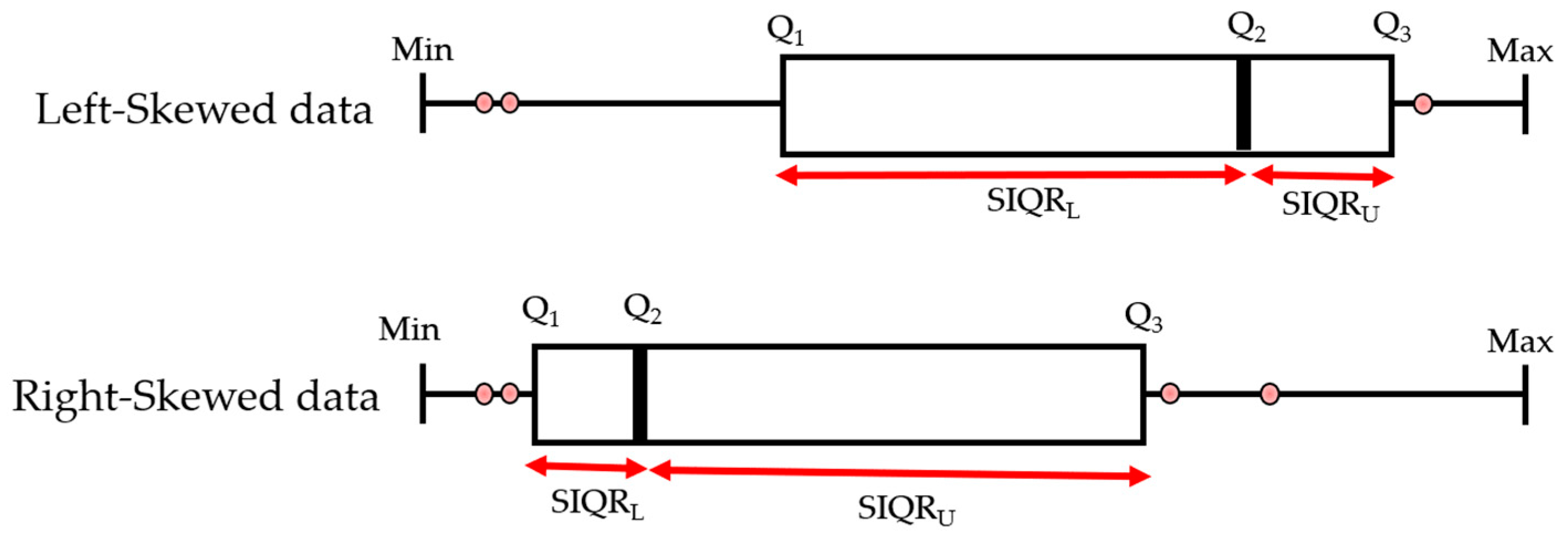
3.1.2. Median-Based Methods

Median-based methods are robust statistic techniques for locating potential outliers, and they utilize the fence labeling approach [47]. One commonly used tool is the median absolute deviation (MAD), which serves as a reliable indicator of data dispersion that is less influenced by extreme values and non-normality (Equation (13)). Two methods, namely, 2MADe and 3MADe, classify values outside the fences as outliers. The lower and upper fences are defined in Equations (14)–(16) [29].

$$MAD=\left[median \left(\left|X_i-median\right|\right)\right]$$

(13)

$$2MA{D}_e method:\{\begin{array}{c}{f}_L=median-2MADe\\ f_U=median+2MADe\end{array}$$

(14)

$$3MA{D}_e method:\{\begin{array}{c}{f}_L=median-3MADe\\ f_U=median+3MADe\end{array}$$

(15)

$$MA{D}_e=1.483\times MAD$$

(16)

Median-based outlier detection methods are utilized in various fields of civil engineering, such as correcting tunnel measurement data, improving hydrological data analysis, and correcting reference points in geodetic and surveying applications [48,49,50].

3.1.3. SD-Based Methods

SD-based methods are basic, straightforward, and simple statistical approaches to detect outliers, and they are considered fence labeling methods. The outliers are screened by calculating the lower and upper cut-off values depending on the mean and standard deviation as defined in Equations (17) and (18) [29,47].

$$2SD Method:\{\begin{array}{c}{f}_l=X_m-2S\\ f_U=X_m+2S\end{array}$$

(17)

$$3SD Method:\{\begin{array}{c}{f}_l=X_m-3S\\ f_U=X_m+3S\end{array}$$

(18)

Another SD-based method is the Z-score method, which shows how many standard deviations a suspicious extreme value is away from the mean value. However, unlike other methods, all datapoints should have their Z-scores calculated first, and those with a Z-score of ±3 are labeled as outliers (Equation (19)).

$$Z_{score}=\frac{x_i-X_m}{S}$$

(19)

For it to be utilized in greatly dispersed datasets, the Z-score was modified such that the mean and standard deviation were replaced by the median and the MAD, which can now be considered a median-based method [51]. In this method, the datapoints with modified Z-scores that exceed ±3.5 are outliers (Equation (20)).

$$Modified Z_{score}=\frac{0.6745 \left(x_i-median\right)}{MAD}$$

(20)

While the SD-based methods can be sensitive to extremities, they have been employed across various disciplines, including civil and petroleum engineering, to accurately identify structural damage via the estimation of signal probability distribution and identification of anomalies [46,52]. These techniques have also been utilized in geotechnical projects to precisely calculate soil parameter uncertainties and treat operational data of tunnel-boring machines [53,54,55]. In petroleum engineering, SD-based methods have successfully identified anomalies in experimental wax deposition values [56]. The modified Z-score method is extensively used in the oil industry to eliminate noise from field test data and reduce input data errors during directional drilling operations in offshore gas fields [57,58].

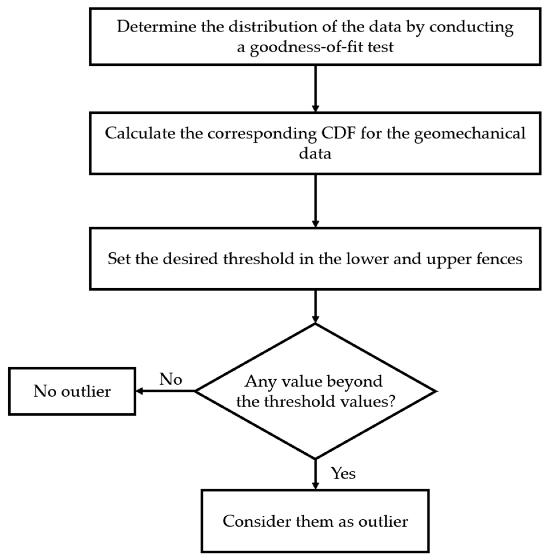
3.1.4. Distribution-Based Approach

Gumbel [59] devised a technique to detect outliers in heavily skewed data where extreme values are far from the majority of datapoints. In this method, the maximum values are assumed to follow the Gumbel distribution [59,60]. To identify outliers, the cumulative distribution function (CDF) of the Gumbel distribution is calculated, and thresholds are specified for the upper and lower fences of the data. Any datapoint that falls outside these fences is considered an outlier and may be investigated further or removed from the dataset (Figure 7). The thresholds are typically based on a desired level of significance or confidence level, such as a probability of 0.05. The approach was later extended to other extreme value distributions, such as the Fréchet, Weibull, and generalized extreme value distributions, by fitting the proper distribution to the data and calculating the related CDF. The method can be used for geomechanical datasets that follow extreme distributions. Choosing the appropriate distribution requires analyzing the data and conducting goodness-of-fit tests such as the Anderson–Darling test or the Kolmogorov–Smirnov test. Although implementing this method may be complex, it indirectly addresses the influence of data skewness by concentrating on the tails of the extreme value distributions.

3.2. Statistical Tests

These methods identify the outliers through statistical hypothesis tests, which are involved with null hypothesis and alternative hypothesis. In general, null hypothesis claims a statement about the data population, while the alternative hypothesis rejects it [4,5,29]. Examining whether an outlier is present in the dataset is possible by using this strategy. Test-based methods mostly rely on standard deviation and assume that the data follow a relatively normal distribution. In this paper, most applicable tests, including Doerffel, Peirce, Chauvenet, Dixon, and Grubbs, are reviewed, which can be applied on geomechanical data.

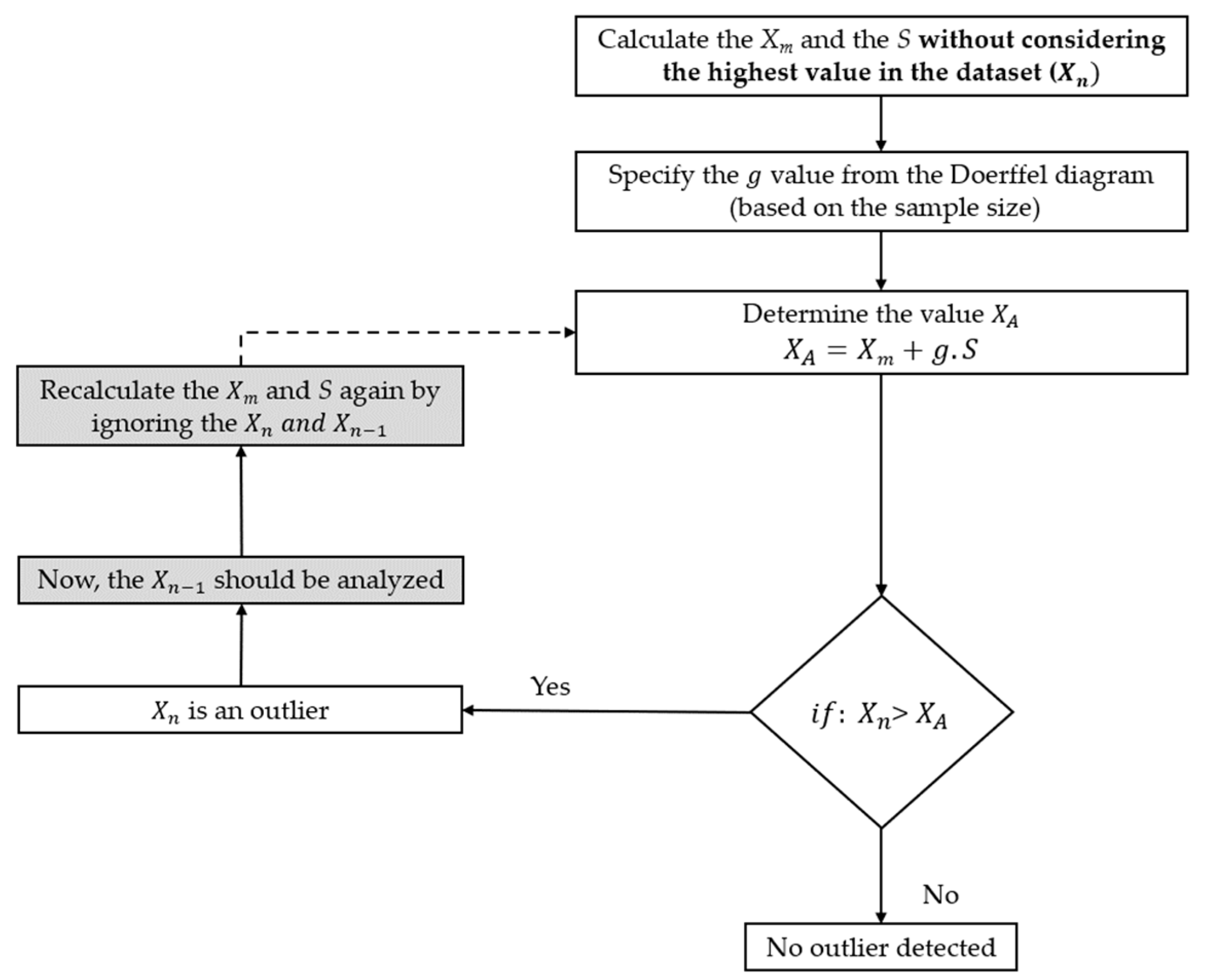
3.2.1. Doerffel’s Test

Doerffel’s test was developed by Doerffel in 1967 to identify high extreme outliers. This test may be less applicable in geomechanical studies because it identifies high extreme outliers only [61]. The method starts by calculating the mean and standard deviation of the dataset regardless of the maximum value (X_n). Then, whether X_n is the outlier or not is checked by determining the threshold value (X_A) (Figure 8). If X_n is identified as an outlier, then the test is re-run, focusing on the second highest value (X_n−1), to identify the next outlier, as illustrated in Figure 6. The $“g”$ parameter of Doerffel’s test can be calculated based on sample size, as shown in Figure 9.

Doerffel’s test is useful in civil and mining engineering across numerous applications. Afraei et al. [62] utilized the technique to treat their rockburst database with confidence in two different scenarios. Moreover, the test has provided a reliable method for determining uncertainty and correcting soil parameters [34]. In mining engineering, this method has also been instrumental in conducting geological data analysis to identify areas that have a high likelihood of containing valuable metal deposits, as evidenced in a study conducted in Iran’s Kivi region [63].

3.2.2. Peirce’s Test

The Peirce criterion is widely acknowledged as the pioneering outlier detection method in the history of statistics for univariate data. It relies on the absolute difference between the extreme value $(x_i)$ and the mean. If the absolute difference is greater than the ($R\times S$), specified in Equation (21), then $x_i$ is an outlier [8]. This test is applicable up to 60 samples only, which was adopted in various fields of study [64]. The relevant equation is shown below:

$$if: \left|x_i-X_m\right|>R\times S \to x_i is an outlier$$

(21)

where “R” is the ratio of the maximum allowable deviation of a datapoint from the mean to the standard deviation (S), which can be obtained from Peirce’s table [65]. Peirce’s test is not commonly utilized in civil and mining engineering, and the literature on the subject is scarce. However, Borosnyói [66] examined the variability of in situ rebound hardness testing of concrete by using Peirce’s test. Additionally, Retamales et al. [67] utilized Peirce’s test to improve fragility curves in a seismic study of a building with cold-formed steel-framed gypsum partition walls.

3.2.3. Chauvenet’s Test

Similar to Peirce’s test, this method uses mean and standard deviation. However, this test is applicable for up to 1000 samples [68]. Chauvenet’s test allows only one run per dataset and involves calculating the standardized deviation from the mean ($\tau$) for an extreme value and comparing it with the critical value (T) of Chauvenet’s table, which is based on the sample size (see Gul et al. [69]). If $\tau$ is greater than T, then this value is flagged as an outlier (Equation (22)) [70].

$$if: \tau =\frac{\left|x_i-X_m\right|}{S}>T \to x_i is an outlier$$

(22)

Chauvenet’s test is widely used in geotechnical engineering to distinguish and eliminate faulty or inconsistent data, such as anomalies of rock strength measurements obtained using the Schmidt hammer test [24,25,26] and reinforced concrete data in laboratory fatigue studies [71,72,73]. The test is also employed in seismic studies to identify and remove outliers from a set of ground motion records (accelerograms) [74], thus making it critical to achieving accurate and reliable results in these applications.

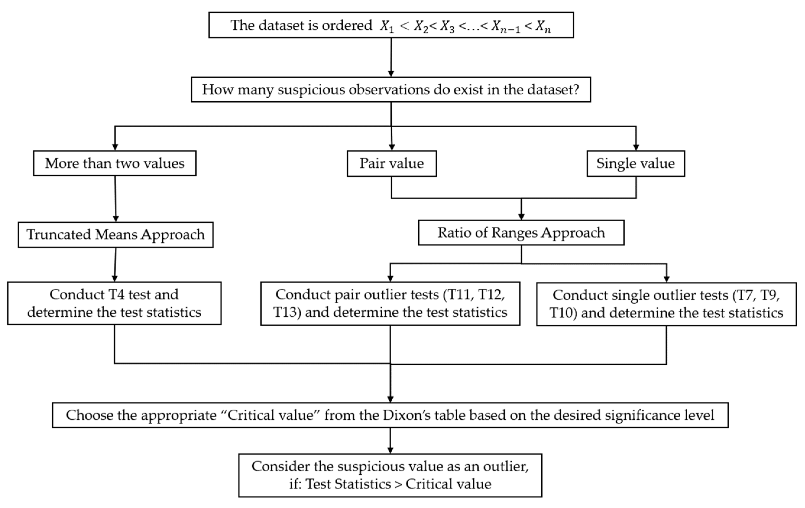
3.2.4. Dixon’s Test

Dixon’s outlier tests have been rarely applied due to the sample size limitation (up to 30) [75]. Verma et al. [76] enhanced these tests by extending the applicability for larger sample sizes up to 1000. The tests are classified in two groups: the ratio of ranges and the truncated means [76]. Figure 10 shows the procedure of Dixon’s tests based on the number of suspicious values. As shown in

Table 2. The proposed relationships for determining the upper- and lower-bound Dixon’s test statistics: the ratio of ranges method (T7, T9-T12) and the truncated means method (T4) [76].

Test Code	Upper-Bound Test Statistic (TS)		Lower-Bound Test Statistic (TS)	Tested Values
T7	$TS7=\frac{X_n-X_{\left(n-1\right)}}{X_n-X_1}$		$\mathrm{Not}\mathrm{Applicable}$	$X_n$
T9	$TS{9}_u=\frac{X_n-X_{\left(n-1\right)}}{X_n-X_2}$		$TS{9}_l=\frac{X_2-X_1}{X_{\left(n-1\right)}-X_1}$	$X_n$, $X_1$
T10	$TS{10}_u=\frac{X_n-X_{\left(n-1\right)}}{X_n-X_3}$		$TS{10}_l=\frac{X_2-X_1}{X_{n-2}-X_1}$	$X_n$, $X_1$
T11	$TS{11}_{up}=\frac{X_n-X_{\left(n-2\right)}}{X_n-X_1}$		$TS{11}_{lp}=\frac{X_3-X_1}{X_n-X_1}$	$X_1$, $X_2,X_n,X_{n-1}$
T12	$TS{12}_{up}=\frac{X_n-X_{\left(n-2\right)}}{X_n-X_2}$		$TS{12}_{lp}=\frac{X_3-X_1}{X_{\left(n-1\right)}-X_1}$	$X_1$, $X_2,X_n,X_{n-1}$
T13	$TS{13}_{up}=\frac{X_n-X_{\left(n-2\right)}}{X_n-X_3}$		$TS{12}_{lp}=\frac{X_3-X_1}{X_{\left(n-2\right)}-X_1}$	$X_1$, $X_2,X_n,X_{n-1}$
T4	Lower bound	$TS{4}_{1l}=\frac{S_1^2}{S^2}, S^2={{\displaystyle \sum }}_{i=1}^{n-1}{\left(X_i-\overline{X}\right)}^2,S_1^2={{\displaystyle \sum }}_{i=2}^n{\left(X_i-{\overline{X}}_1^{}\right)}^2,\left[\overline{X}=\frac{{{\displaystyle \sum }}_{i=1}^n{X}_i}{n},{\overline{X}}_1^{}=\frac{{{\displaystyle \sum }}_{i=2}^n{X}_i}{n-1}\right]$		$X_1$
		$TS{4}_{2l}=\frac{S_{\left(1,2\right)}^2}{S^2}, S_{\left(1,2\right)}^2={{\displaystyle \sum }}_{i=3}^n{\left(X_i-{\overline{X}}_{\left(1,2\right)}^{}\right)}^2,\left[{\overline{X}}_{\left(1,2\right)}^{}=\frac{{{\displaystyle \sum }}_{i=3}^n{X}_i}{n-2}\right]$		$X_1$, $X_2$
		$TS{4}_{3l}=\frac{S_{\left(1,2,3\right)}^2}{S^2}, S_{\left(1,2,3\right)}^2={{\displaystyle \sum }}_{i=4}^n{\left(X_i-{\overline{X}}_{\left(1,2,3\right)}^{}\right)}^2,\left[{\overline{X}}_{\left(1,2,3\right)}^{}=\frac{{{\displaystyle \sum }}_{i=4}^n{X}_i}{n-3}\right]$		$X_1$, $X_2$, $X_3$
		$TS{4}_{4l}=\frac{S_{\left(1,2,3,4\right)}^2}{S^2},$ $S_{\left(1,2,3,4\right)}^2={{\displaystyle \sum }}_{i=5}^n{\left(X_i-{\overline{X}}_{\left(1,2,3,4\right)}^{}\right)}^2, \left[{\overline{X}}_{\left(1,2,3,4\right)}^{}=\frac{{{\displaystyle \sum }}_{i=5}^n{X}_i}{n-4}\right]$		$X_1$, $X_2$, $X_3,X_4$
	Upper bound	$$\begin{gathered} TS{4}_{1u}=\frac{S_n^2}{S^2}, S^2={{\displaystyle \sum }}_{i=1}^{n-1}{\left(X_i-\overline{X}\right)}^2,S_n^2 \\ \hspace{1em}\hspace{1em}\hspace{1em}\hspace{1em}\hspace{1em}\hspace{1em}={{\displaystyle \sum }}_{i=1}^{n-1}{\left(X_i-{\overline{X}}_n^{}\right)}^2,\left[\overline{X}=\frac{{{\displaystyle \sum }}_{i=1}^n{X}_i}{n},{\overline{X}}_n^{}=\frac{{{\displaystyle \sum }}_{i=1}^{n-1}{X}_i}{n-1}\right] \end{gathered}$$		$X_n$
		$TS{4}_{2u}=\frac{S_{\left(n,n-1\right)}^2}{S^2},S_{\left(n,n-1\right)}^2={{\displaystyle \sum }}_{i=1}^{n-2}{\left(X_i-{\overline{X}}_{\left(n,n-1\right)}^{}\right)}^2,\left[{\overline{X}}_{\left(n,n-1\right)}^{}=\frac{{{\displaystyle \sum }}_{i=1}^{n-2}{X}_i}{n-2}\right]$		$X_n$, $X_{n-1}$
		$$\begin{gathered} TS{4}_{3u}=\frac{S_{\left(n,n-1,n-2\right)}^2}{S^2},, S_{\left(n,n-1,n-2\right)}^2 \\ \hspace{1em}\hspace{1em}\hspace{1em}\hspace{1em}\hspace{1em}={{\displaystyle \sum }}_{i=1}^{n-3}{\left(X_i-{\overline{X}}_{\left(n,n-1,n-2\right)}^{}\right)}^2,\left[{\overline{X}}_{\left(n,n-1,n-2\right)}^{}=\frac{{{\displaystyle \sum }}_{i=1}^{n-3}{X}_i}{n-3}\right] \end{gathered}$$		$X_n$, $X_{n-1}$, $X_{n-2}$
		$$\begin{gathered} TS{4}_{4u}=\frac{S_{\left(n,n-1,n-2,n-3\right)}^2}{S^2},, S_{\left(n,n-1,n-2,n-3\right)}^2 \\ \hspace{1em}\hspace{1em}\hspace{1em}\hspace{1em}\hspace{1em}={{\displaystyle \sum }}_{i=1}^{n-4}{\left(X_i-{\overline{X}}_{\left(n,n-1,n-2,n-3\right)}^{}\right)}^2,\left[{\overline{X}}_{\left(n,n-1,n-2,n-3\right)}^{}=\frac{{{\displaystyle \sum }}_{i=1}^{n-4}{X}_i}{n-4}\right] \end{gathered}$$		$X_n$, $X_{n-1}$, $X_{n-2},X_{n-3}$

The presented subscripts $u$, $l$, $up$, and $lp$ are upper, lower, upper pair, and lower pair values, respectively.

, the test statistics (TS) in each test is determined and compared with the associated critical values, as calculated by Appendix in Verma et al. [76]. Similar to other test-based methods, if the TS is greater than the critical value, then the suspicious value is an outlier.

Dixon’s test is not commonly used in civil and mining engineering, but it can effectively identify and remove outliers in water engineering data, particularly in piezometric measurements [77]. Kim et al. [78] evaluated soil data accuracy by using this test, thus facilitating statistical adjustments that help improve engineering decisions.

3.2.5. Grubbs’ Test

Grubbs [79] introduced a deviation-based approach that assumes a normality for the data, which is why it may be less appropriate for non-normal datasets. The outliers are detected by calculating the test statistics ($G_{statistics})$ for the lower and upper bounds by using mean and standard deviation. As shown in Equations (23) and (24), x₁ and x_n are minimum and maximum values in the dataset, respectively, which are called outliers if their $G_{statistics}$ are greater than the associated critical values. Grubbs’ test does not have a sample size limitation for calculating the critical values ($G_{critical}$), and they can be determined for various confidence levels $\left(\alpha \right)$ so that the datasets can be analyzed by considering different probabilities (see Equation (25)) [79]. In Equation (25), “t” and n are the value of the Student’s t-distribution and the sample size, respectively.

$$For lower bound \to G_{statistic}=\frac{X_m-x_1}{S}$$

(23)

$$For upper bound \to G_{statistic}=\frac{x_n-X_m}{S}$$

(24)

$$G_{Critical}=\frac{\left(n-1\right)}{\sqrt{n}}\sqrt{\frac{t_{\left(\alpha /n,n-2\right)}^2}{n-2+t_{\left(\alpha /n,n-2\right)}^2}}$$

(25)

Several geomechanical studies applied Grubbs’ test [80]. In the underground mining field, this test was conducted to treat the hang-up and secondary breaking vulnerability data collected for drawpoints in a mining operation, ensuring more accurate results [81]. In addition, this method was successfully utilized to correct in situ cone geotechnical tests and evaluate the shear strength parameters in triaxial testing [82,83].

4. Evaluation of Applicability of Outlier Methods in Geomechanics

In geomechanical data, the selection of best outlier detection method should be accompanied by an engineering judgment considering the characteristics of the data and the desired outcome of the analysis. As illustrated in Figure 11, when the suitability of using outlier detection methods for analyzing geomechanical data is assessed, several key factors should be taken into consideration.

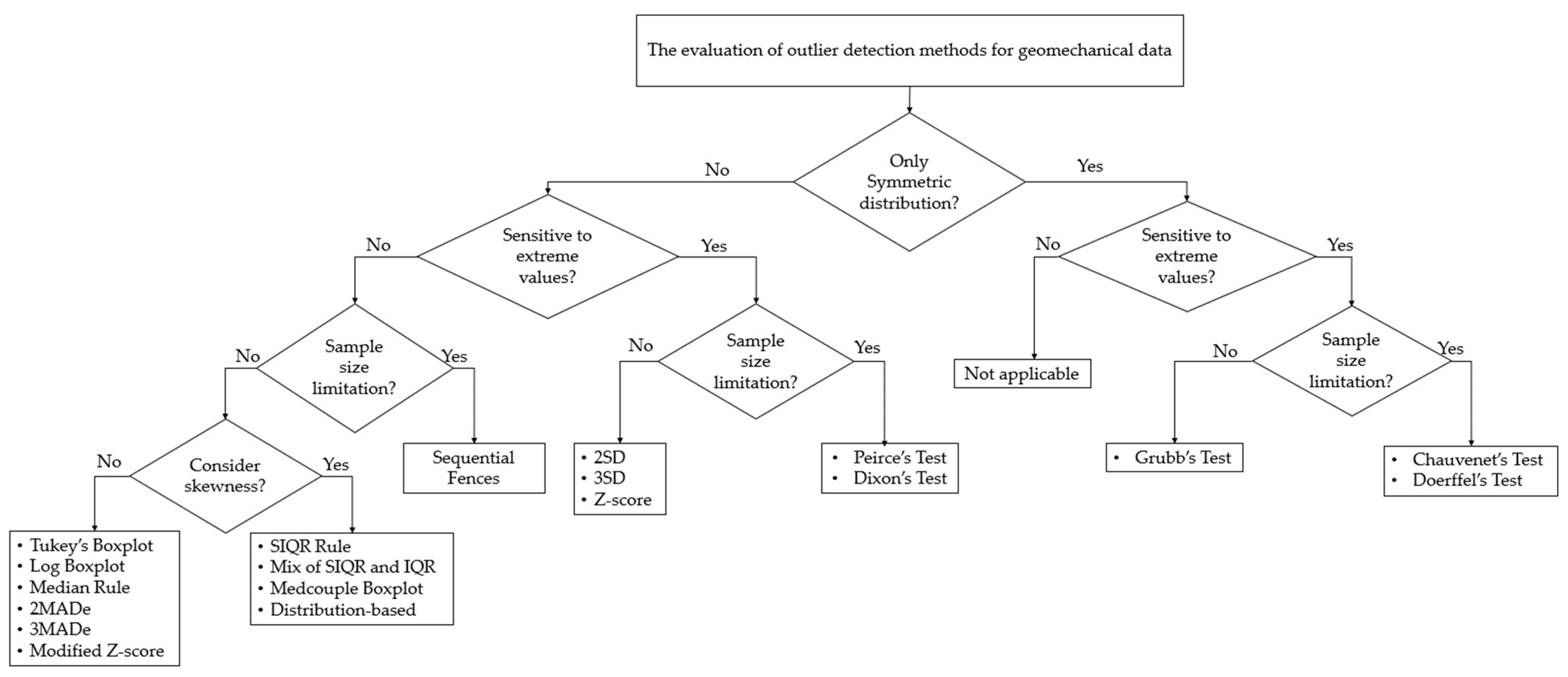
• An important factor to consider in the suitability of outlier detection methods is the shape of data distribution. Geomechanical data are generally assumed to be normally distributed. In reality, however, laboratory test results such as UCS values naturally show large variations, which leads them to be greatly skewed. Thus, the visual shape of the data frequencies should be primarily analyzed. Certain outlier detection methods, such as Doerffel, Chauvenet, and Grubbs, are suitable for symmetrically distributed data only [38,68,79]. Many of the most applicable methods can be used for either symmetric or asymmetric distributions. Although most fence labeling methods do not explicitly consider the data distribution, they rely on several statistics that are related to the distribution. Therefore, methods with no distribution limitations may be better suited for geomechanical data.
• When outlier detection methods are evaluated, their sensitivity to extreme values is an important detail to consider. Deviation-based outlier methods, which incorporate standard deviation in their formulas, are more sensitive to the presence of extreme values in the dataset [4,37]. Thus, they may not be suitable for analyzing geomechanical data. However, some approaches such as IQR-based methods exhibit robustness against outliers. In addition, methods that use the median value instead of the mean value are generally less susceptible to violations of the dataset [35].
• The number of samples in a geomechanical dataset also affects the applicability of outlier detection methods. While geomechanical datasets may not have a large number of samples, certain statistical tests such as Peirce’s test cannot be applied to sample sizes greater than 60 [29]. For larger datasets, IQR- and median-based methods are more suitable because they can be applied to any sample size without being influenced by extreme datapoints [36].
• Geomechanical data tend to be skewed because of their significant inherent variability, which is why a proper outlier method should address the effect of skewness. However, there are a few methods such as MC boxplot, SIQR rule, and the mix of the SIQR and IQR methods which consider the skewness by modifying the fences [31,41]. Furthermore, the distribution-based approach indirectly takes the data skewness into account because it focuses on the distribution tails and can identify extreme outliers that are far away from the rest of the data. However, many outlier methods are still used for heavily skewed data.

Comparison of Various Outlier Detection Methods

To compare the performance of the methods, we applied the reviewed outlier detection methods on actual data of the uniaxial compressive strength (UCS) of rock samples extracted from Westwood Mine in Quebec, Canada. Figure 12 represents the process of the UCS test on a rock sample. The dataset comprised 157 samples with a wide range of values, spanning from 32.10 MPa to 371.10 MPa. In the selection of an appropriate outlier detection method for UCS data, an important detail to consider is the expected mechanical behavior of the rock type in the dataset, which in this case consists of metamorphic rocks.

Table 3. The results of outlier detection methods applied on the actual UCS dataset (note: LB and UB are the lower and upper bounds of the dataset, respectively).

Outlier Detection Method	Confidence Interval (MPa)	Number of Outliers
		LB	UB
Tukey’s boxplot (1.5 IQR)	26.10 < UCS < 266.10	0	10
Tukey’s boxplot (3.0 IQR)	−63.90 < UCS < 356.10	0	1
Tukey’s boxplot (2.2 IQR)	−15.90 < UCS < 308.10	0	2
Log boxplot	15.34 < UCS < 276.86	0	5
Sequential fences	NA *	NA	NA
Median rule	11.80 < UCS < 287.80	0	4
MC boxplot	32.29 < UCS < 271.04	0	8
SIQR rule	15.00 < UCS < 255.00	0	11
Mix of SIQR and IQR	0.78 < UCS < 246.34	0	13
2MADe method	49.85 < UCS < 249.75	3	12
3MADe method	−0.13 < UCS < 349.71	0	1
2SD method	40.86 < UCS < 270.30	1	8
3SD method	−16.50 < UCS < 327.67	0	2
Z-score	−3.00 < Z-score < +3.00	0	2
Modified Z-score	−3.50 < modified Z-score < +3.50	0	2
Distribution-based approach	43.15 < UCS < 268.00	1	9
Doerffel’s test	Statistical tests identify outliers based on statistical hypotheses	NA	1
Peirce’s test		NA	NA
Chauvenet’s test		0	1
Dixon’s test (ratio of ranges)		0	0
Dixon’s test (truncated means)		4	0
Grubbs’ test		NA	NA

* Not applicable.

presents the results of all outlier detection methods applied on the UCS data. After applying all outlier methods on the UCS data, we have utilized the confidence interval of each method to draw a comparison among the various methods. The confidence interval indicates a reliable range of UCS values, with any values falling outside this range being considered as outliers. Methods such as Peirce and sequential fences were unsuitable for the UCS data because of the large sample size. However, in the selection of appropriate methods for the UCS data, the lower and upper threshold values should be aligned with rock mechanics principles because negative UCS values are meaningless. As illustrated in Figure 13, certain methods, such as Tukey’s boxplot (using 3 IQR and 2.2 IQR), 3MADe, and 3SD, may not be able to detect outliers in the lower threshold due to their negative value. Therefore, rock mechanics principles are of great importance in determining the more suitable methods for the geomechanical data. In addition, the suggested lower threshold of the UCS value (0.78) estimated by the modified boxplot (mix of SIQR and IQR method) may not represent a reasonable UCS value for a rock sample. However, the MC boxplot, 2MADe, and 2SD methods provided reasonable thresholds, namely, 32.29 < UCS < 271.04, 49.85 < UCS < 249.75, and 40.86 < UCS < 270.30, respectively. We also applied the distribution-based method on the UCS data. In this method, we first conducted the Anderson–Darling goodness-of-fit test to determine the most fitted distributions for the dataset. The test showed that the data follow normal and logistic distributions. Then, we determined the associated CDF graphs, as illustrated in Figure 14. The threshold values of UCS (fences) should be computed based on the confidence level (0.05) to identify the outliers, and datapoints beyond this range were assumed as outliers, as presented in Table 3. The calculated confidence interval of the distribution-based method seems logical. In statistical tests, we may only use the number of detected outliers of each method to select the most appropriate outlier technique. However, we observed that Doerffel’s test was not able to detect outliers in the lower threshold, which is a vital limitation for an outlier method to treat the geomechanical data. Several methods, such as Dixon (ratio of ranges), Chauvenet, Z-score, and modified Z-score, were too conservative in labeling the outliers, as they rarely considered the extreme UCS values as outliers.

Notably, the selection of appropriate software for identifying outliers in geomechanical datasets depends on the practitioner’s specific requirements and preferences, as well as the complexity of the data and the outlier detection method employed. Various computer programs offer built-in functions for outlier detection, such as boxplots, Z-scores, and modified Z-scores, which can facilitate the data treatment process and aid geomechanical practitioners in identifying outliers in their laboratory or field data. Popular software options in geomechanics include Microsoft Excel and its @Risk add-in tool, Minitab, SPSS, and MATLAB [84,85,86,87].

5. Discussion

Data treatment processes and outlier detection methods can sometimes be undervalued in geomechanical projects where there may not be a significant amount of lab data to analyze. However, inaccurate or unreliable data can lead to faulty design decisions that increase the risk of safety hazards, project delays, and catastrophic failure. Conducting tests on rock samples is costly, but making design decisions on inaccurate data can incur even higher costs. Therefore, an essential step for engineers and practitioners is to prioritize the data treatment process, including the selection of appropriate outlier detection methods in geomechanical projects. By using appropriate outlier detection methods, engineers can obtain a more accurate representation of the true range of variation in their data and make more informed design decisions. This approach can lead to more efficient designs and cost savings without compromising safety or reliability.

The selection of an appropriate outlier detection method in geomechanical projects depends on various factors such as data distribution, sample size, and other considerations. Each method has its own advantages and disadvantages. Statistical methods rely on a statistical model of the data and hypothesis testing to determine whether a data point is an outlier or not. One of the main advantages of statistical methods is their ability to provide a clear statistical basis for identifying outliers, which is particularly useful when dealing with large datasets. However, certain statistical tests such as Peirce and Grubbs are not suitable for large sample sizes, while Doerffel’s test cannot detect outliers in the lower bound, which can be a significant drawback. In addition, statistical techniques have limitations with non-symmetrical or skewed data distribution, thus posing challenges to the selection of an appropriate statistical model, which may result in misidentifying outliers.

Conversely, fence labeling methods are often popular among geomechanical practitioners because they mostly provide graphical representations, such as boxplots or scatterplots, rather than relying solely on statistical methods. These methods can also be robust to large data variations, especially the ones that use the median and MAD as tools to define the fences.

Geomechanical datasets can often exhibit significant uncertainties because of the complex nature of rock formation, making IQR- and median-based methods particularly suitable for identifying outliers. Accurate analysis and characterization of rock properties depend on the identification and treatment of outliers, making outlier detection methods an essential part of geomechanical data analysis. When dealing with normally distributed data, SD-based methods are simple and user-friendly options for detecting outliers in geomechanical data. However, if the data do not follow a normal distribution, then distribution-based methods may be more effective because they identify outliers on the basis of the behavior of extreme values and are thus a useful tool for datasets with skewed or heavy-tailed distributions.

The IQR-based methods are well known in geomechanics, with Tukey’s boxplot being a popular tool because of its ability to provide a visual representation of the data distribution, which makes identifying outliers and understanding the overall pattern of the data easier. However, Tukey’s boxplot has limitations because it relies on a single fence to identify outliers, which may not be suitable for certain geomechanical datasets. Modified boxplots such as the sequential fences method have been developed to address this issue.

The sequential fences method facilitates the creation of multiple fences for the data, potentially providing more reliable identification of outliers. By utilizing a sequence of fences, the sequential fences method can better capture the distribution of the data and identify outliers that may be missed by other methods. However, the sequential fences method is limited to datasets with a sample size of less than 100.

Furthermore, the traditional boxplot has a limitation in heavily skewed data because it does not consider the skewness. Modified boxplots are designed to address the limitations of traditional boxplots by incorporating robust tools such as the SIQR or MC function, which allow the skewness and definition of fence limits to be computed. This approach is particularly beneficial in the case of heavily skewed data because it can provide practitioners with more accurate results. Modified boxplots are more sensitive to outliers than traditional boxplots because they can identify outliers located far from the median or in the tails of the distribution. However, constructing and interpreting modified boxplots may require more advanced statistical techniques.

6. Conclusions

In this review, we thoroughly analyzed various outlier detection methods available in the literature and proposed a methodology for categorizing and assessing their suitability for geomechanical data. We classified the outlier detection methods into two main categories: fence labeling methods and statistical tests. Fence labeling methods identify outliers by defining upper and lower thresholds and by considering any data point outside this range as an outlier. Statistical tests utilize hypothesis testing by comparing the test statistics with the corresponding critical value to identify outliers.

An important detail to note is that the effectiveness of these methods largely depends on the nature of geomechanical data and requires engineering judgment to determine the most appropriate method. Therefore, a recommended approach when choosing an appropriate outlier detection method is to consider the specific characteristics of the data. We also developed a flowchart to guide geomechanical practitioners in selecting the appropriate outlier detection method based on their specific needs and the complexity of their data. This flowchart takes into account important considerations for geomechanical data and can be used as a helpful tool for practitioners in identifying outliers in their laboratory or field data.

The applicability of these methods in geomechanical data has been evaluated, and we found that statistical tests are not as effective in detecting outliers, because of their inability to handle skewed data and limited sample sizes. However, modified IQR-based methods, such as the MC boxplot and SIQR rule, appear to be the most accurate outlier detection methods in geomechanical data because they take into account the significant impact of skewness in outlier detection. This review paper provides valuable insights into the selection and application of outlier detection methods for geomechanical data, thus possibly facilitating accurate data analysis and interpretation. Future research can further investigate and improve upon these findings to develop more robust and effective outlier detection methods for geomechanical data.

References

- Mazraehli, M.; Zare, S. An application of uncertainty analysis to rock mass properties characterization at porphyry copper mines. Bull. Eng. Geol. Environ. 2020, 79, 3721–3739. [Google Scholar] [CrossRef]
- Han, L.; Wang, L.; Zhang, W. Quantification of statistical uncertainties of rock strength parameters using Bayesian-based Markov Chain Monte Carlo method. In Proceedings of the IOP Conference Series: Earth and Environmental Science, Beijing, China, 19–21 November 2020; IOP Publishing: Bristol, UK, 2020; Volume 570, p. 032051. [Google Scholar]
- Connor Langford, J.; Diederichs, M.S. Quantifying uncertainty in Hoek–Brown intact strength envelopes. Int. J. Rock Mech. Min. Sci. 2015, 74, 91–102. [Google Scholar] [CrossRef]
- Barbato, G.; Barini, E.; Genta, G.; Levi, R. Features and performance of some outlier detection methods. J. Appl. Stat. 2011, 38, 2133–2149. [Google Scholar] [CrossRef]
- Saleem, S.; Aslam, M.; Shaukat, M.R. A review and empirical comparison of univariate outlier detection methods. Pak. J. Stat. 2021, 37, 447–462. [Google Scholar]
- Kannan, K.S.; Manoj, K.; Arumugam, S. Labeling methods for identifying outliers. Int. J. Stat. Syst. 2015, 10, 231–238. [Google Scholar]
- Hadi, A.S.; Imon, A.R.; Werner, M. Detection of outliers. Wiley Interdiscip. Rev. Comput. Stat. 2009, 1, 57–70. [Google Scholar] [CrossRef]
- Peirce, B. Criterion for the rejection of doubtful observations. Astron. J. 1852, 2, 161–163. [Google Scholar] [CrossRef]
- Tiryaki, B. Predicting intact rock strength for mechanical excavation using multivariate statistics, artificial neural networks, and regression trees. Eng. Geol. 2008, 99, 51–60. [Google Scholar] [CrossRef]
- Heidarzadeh, S.; Saeidi, A.; Lavoie, C.; Rouleau, A. Geomechanical characterization of a heterogenous rock mass using geological and laboratory test results: A case study of the Niobec Mine, Quebec (Canada). SN Appl. Sci. 2021, 3, 640. [Google Scholar] [CrossRef]
- Shirani Faradonbeh, R.; Taheri, A.; Karakus, M. The propensity of the over-stressed rock masses to different failure mechanisms based on a hybrid probabilistic approach. Tunn. Undergr. Space Technol. 2022, 119, 104214. [Google Scholar] [CrossRef]
- Bozorgzadeh, N.; Dolowy-Busch, M.; Harrison, J.P. Obtaining Robust Estimates of Rock Strength for Rock Engineering Design. In Proceedings of the 13th ISRM International Congress of Rock Mechanics, Montreal, QC, Canada, 10–13 May 2015. [Google Scholar]
- Xue, Y.; Bai, C.; Qiu, D.; Kong, F.; Li, Z. Predicting rockburst with database using particle swarm optimization and extreme learning machine. Tunn. Undergr. Space Technol. 2020, 98, 103287. [Google Scholar] [CrossRef]
- Roy, J.; Eberhardt, E.; Bewick, R.; Campbell, R. Application of Data Analysis Techniques to Identify Rockburst Mechanisms, Triggers, and Contributing Factors in Cave Mining. Rock Mech. Rock Eng. 2023, 56, 2967–3002. [Google Scholar] [CrossRef]
- Zhang, Q.; Liu, C.; Guo, S.; Wang, W.; Luo, H. Evaluation of rock burst intensity of cloud model based on CRITIC method and order relation analysis method. Res. Sq. 2022. [Google Scholar] [CrossRef]
- Lin, S.; Zheng, H.; Han, C.; Han, B.; Li, W. Evaluation and prediction of slope stability using machine learning approaches. Front. Struct. Civ. Eng. 2021, 15, 821–833. [Google Scholar] [CrossRef]
- Manouchehrian, A.; Gholamnejad, J.; Sharifzadeh, M. Development of a model for analysis of slope stability for circular mode failure using genetic algorithm. Environ. Earth Sci. 2014, 71, 1267–1277. [Google Scholar] [CrossRef]
- Zhou, J.; Li, E.; Yang, S.; Wang, M.; Shi, X.; Yao, S.; Mitri, H.S. Slope stability prediction for circular mode failure using gradient boosting machine approach based on an updated database of case histories. Saf. Sci. 2019, 118, 505–518. [Google Scholar] [CrossRef]
- Tomaszewski, D.; Rapiński, J.; Stolecki, L.; Śmieja, M. Switching Edge Detector as a tool for seismic events detection based on GNSS timeseries. Arch. Min. Sci. 2022, 67, 317–332. [Google Scholar]
- Hunt, R.E. Geotechnical Engineering Investigation Handbook; CRC Press: Boca Raton, FL, USA, 2005. [Google Scholar]
- Pan, J.; Bai, Z.; Cao, Y.; Zhou, W.; Wang, J. Influence of soil physical properties and vegetation coverage at different slope aspects in a reclaimed dump. Environ. Sci. Pollut. Res. 2017, 24, 23953–23965. [Google Scholar] [CrossRef]
- Shao, Z.; Armaghani, D.J.; Bejarbaneh, B.Y.; Mu’azu, M.; Mohamad, E.T. Estimating the friction angle of black shale core specimens with hybrid-ANN approaches. Measurement 2019, 145, 744–755. [Google Scholar] [CrossRef]
- Li, S.; Wang, Y.; Xie, X. Prediction of Uniaxial Compression Strength of Limestone Based on the Point Load Strength and SVM Model. Minerals 2021, 11, 1387. [Google Scholar] [CrossRef]
- Bolla, A.; Paronuzzi, P. UCS field estimation of intact rock using the Schmidt hammer: A new empirical approach. In Proceedings of the IOP Conference Series: Earth and Environmental Science, Turin, Italy, 20–25 September 2021; p. 012014. [Google Scholar]
- Goktan, R.; Gunes, N. A comparative study of Schmidt hammer testing procedures with reference to rock cutting machine performance prediction. Int. J. Rock Mech. Min. Sci. 2005, 42, 466–472. [Google Scholar] [CrossRef]
- Goktan, R.; Ayday, C. A suggested improvement to the Schmidt rebound hardness ISRM suggested method with particular reference to rock machineability. Int. J. Rock Mech. Min. Sci. 1993, 30, 321–322. [Google Scholar] [CrossRef]
- Dindarloo, S.R.; Siami-Irdemoosa, E. Maximum surface settlement based classification of shallow tunnels in soft ground. Tunn. Undergr. Space Technol. 2015, 49, 320–327. [Google Scholar] [CrossRef]
- Carmona, S.; Molins, C.; Aguado, A.; Mora, F. Distribution of fibers in SFRC segments for tunnel linings. Tunn. Undergr. Space Technol. 2016, 51, 238–249. [Google Scholar] [CrossRef]
- Seo, S. A Review and Comparison of Methods for Detecting Outliers in Univariate Data Sets. Master’s Thesis, University of Pittsburgh, Pittsburgh, PA, USA, 2006. [Google Scholar]
- Tukey, J.W. Exploratory Data Analysis; Addison-wesley series in behavioral science-quantitative methods; Addison-Wesley: Reading, MA, USA, 1977. [Google Scholar]
- Walker, M.L.; Dovoedo, Y.H.; Chakraborti, S.; Hilton, C.W. An Improved Boxplot for Univariate Data. Am. Stat. 2018, 72, 348–353. [Google Scholar] [CrossRef]
- Petrone, P.; Allocca, V.; Fusco, F.; Incontri, P.; De Vita, P. Engineering geological 3D modeling and geotechnical characterization in the framework of technical rules for geotechnical design: The case study of the Nola’s logistic plant (southern Italy). Bull. Eng. Geol. Environ. 2023, 82, 12. [Google Scholar] [CrossRef]
- Almeida, A.P.; Liu, J. Statistical evaluation of design methods for micropiles in Ontario soils. DFI J. J. Deep Found. Inst. 2018, 12, 133–146. [Google Scholar] [CrossRef]
- Sanou, A.-G.; Saeidi, A.; Heidarzadeh, S.; Chavali, R.V.P.; Samti, H.E.; Rouleau, A. Geotechnical Parameters of Landslide-Prone Laflamme Sea Deposits, Canada: Uncertainties and Correlations. Geosciences 2022, 12, 297. [Google Scholar] [CrossRef]
- Hoaglin, D.C.; Iglewicz, B. Fine-Tuning Some Resistant Rules for Outlier Labeling. J. Am. Stat. Assoc. 1987, 82, 1147–1149. [Google Scholar] [CrossRef]
- Dawson, R. How significant is a boxplot outlier? J. Stat. Educ. 2011. [Google Scholar] [CrossRef]
- Gignac, G. How2statsbook (Online Edition 1), Chapter 2; Perth, Australia. 2019. Available online: https://www.how2statsbook.com (accessed on 29 March 2023).
- Schwertman, N.C.; de Silva, R. Identifying outliers with sequential fences. Comput. Stat. Data Anal. 2007, 51, 3800–3810. [Google Scholar] [CrossRef]
- Carling, K. Resistant outlier rules and the non-Gaussian case. Comput. Stat. Data Anal. 2000, 33, 249–258. [Google Scholar] [CrossRef]
- Kimber, A. Exploratory data analysis for possibly censored data from skewed distributions. J. R. Stat. Soc. Ser. C Appl. Stat. 1990, 39, 21–30. [Google Scholar] [CrossRef]
- Hubert, M.; Vandervieren, E. An adjusted boxplot for skewed distributions. Comput. Stat. Data Anal. 2008, 52, 5186–5201. [Google Scholar] [CrossRef]
- Barnett, O.; Cohen, A. The histogram and boxplot for the display of lifetime data. J. Comput. Graph. Stat. 2000, 9, 759–778. [Google Scholar]
- Dovoedo, Y.; Chakraborti, S. Boxplot-based outlier detection for the location-scale family. Commun. Stat. Simul. Comput. 2015, 44, 1492–1513. [Google Scholar] [CrossRef]
- Romão, X.; Vasanelli, E. Identification and Processing of Outliers. In Non-Destructive In Situ Strength Assessment of Concrete: Practical Application of the RILEM TC 249-ISC Recommendations; Springer: Berlin/Heidelberg, Germany, 2021; pp. 161–180. [Google Scholar]
- Yang, M.; Wang, R.; Li, M.; Liao, M. A PSI targets characterization approach to interpreting surface displacement signals: A case study of the Shanghai metro tunnels. Remote Sens. Environ. 2022, 280, 113150. [Google Scholar] [CrossRef]
- Azad, S.T.; Moghaddassi, N.; Sayehbani, M. Digital Shoreline Analysis System improvement for uncertain data detection in measurements. Environ. Monit. Assess. 2022, 194, 646. [Google Scholar] [CrossRef]
- Olewuezi, N. Note on the comparison of some outlier labeling techniques. J. Math. Stat. 2011, 7, 353–355. [Google Scholar]
- Duchnowski, R. Median-based estimates and their application in controlling reference mark stability. J. Surv. Eng. 2010, 136, 47–52. [Google Scholar] [CrossRef]
- Hussain, I.; Uddin, M. Functional and multivariate hydrological data visualization and outlier detection of Sukkur Barrage. Int. J. Comput. Appl. 2019, 178, 20–29. [Google Scholar] [CrossRef]
- Choi, S.-I.; Shim, S.; Kong, S.-M.; Kim, Y.B.; Lee, S.-W. Efficiency Analysis of Filter-Based Calibration Technique to Improve Tunnel Measurement Reliability. KSCE J. Civ. Eng. 2022, 26, 2926–2938. [Google Scholar] [CrossRef]
- Iglewicz, B.; Hoaglin, D.C. How to Detect and Handle Outliers; Asq Press: Milwaukee, WI, USA, 1993; Volume 16. [Google Scholar]
- Wah, W.S.L.; Owen, J.S.; Chen, Y.-T.; Elamin, A.; Roberts, G.W. Removal of masking effect for damage detection of structures. Eng. Struct. 2019, 183, 646–661. [Google Scholar]
- Kottegoda, N.T.; Rosso, R. Applied Statistics for Civil and Environmental Engineers; Blackwell Publishing: Hoboken, NJ, USA, 2008. [Google Scholar]
- Kor, K.; Ertekin, S.; Yamanlar, S.; Altun, G. Penetration rate prediction in heterogeneous formations: A geomechanical approach through machine learning. J. Pet. Sci. Eng. 2021, 207, 109138. [Google Scholar] [CrossRef]
- Yang, H.; Song, K.; Zhou, J. Automated recognition model of geomechanical information based on operational data of tunneling boring machines. Rock Mech. Rock Eng. 2022, 55, 1499–1516. [Google Scholar] [CrossRef]
- Kamari, A.; Khaksar-Manshad, A.; Gharagheizi, F.; Mohammadi, A.H.; Ashoori, S. Robust model for the determination of wax deposition in oil systems. Ind. Eng. Chem. Res. 2013, 52, 15664–15672. [Google Scholar] [CrossRef]
- Monteiro, D.D.; Duque, M.M.; Chaves, G.S.; Ferreira Filho, V.M.; Baioco, J.S. Using data analytics to quantify the impact of production test uncertainty on oil flow rate forecast. Oil Gas Sci. Technol. Rev. D’ifp Energ. Nouv. 2020, 75, 7. [Google Scholar] [CrossRef]
- Shaygan, K.; Jamshidi, S. Prediction of rate of penetration in directional drilling using data mining techniques. Geoenergy Sci. Eng. 2023, 221, 111293. [Google Scholar] [CrossRef]
- Gumbel, E. Statistics of Extremes; Columbia University Press: New York, NY, USA, 1958. [Google Scholar]
- Barnett, V.; Lewis, T. Outliers in Statistical Data; Wiley: New York, NY, USA, 1994; Volume 3. [Google Scholar]
- Doerffel, K. Die Statistische Auswertung von Analysenergebnissen; Springer: Berlin, Germany, 1967; Volume 2. [Google Scholar]
- Afraei, S.; Shahriar, K.; Madani, S.H. Statistical analysis of rock-burst events in underground mines and excavations to present reasonable data-driven predictors. J. Stat. Comput. Simul. 2017, 87, 3336–3376. [Google Scholar] [CrossRef]
- Adel, S.; Mansour, Z.; Ardeshir, H. Geochemical behavior investigation based on k-means and artificial neural network prediction for titanium and zinc, Kivi region, Iran. Bull. Tomsk Polytech. Univ. Geo Assets Eng. 2021, 332, 113–125. [Google Scholar]
- Rochim, A.F.R.F. Chauvenet’s Criterion, Peirce’s Criterion, and Thompson’s Criterion (Literatures Review). Available online: https://www.researchgate.net/publication/299829851 (accessed on 21 March 2016).
- Ross, S.M. Peirce’s criterion for the elimination of suspect experimental data. J. Eng. Technol. 2003, 20, 38–41. [Google Scholar]
- Borosnyói, A. Variability case study based on in-situ rebound hardness testing of concrete: Part 1. Statistical analysis of inherent variability parameters. Építöanyag (Online) 2014, 66, 85. [Google Scholar] [CrossRef]
- Retamales, R.; Davies, R.; Mosqueda, G.; Filiatrault, A. Experimental seismic fragility of cold-formed steel framed gypsum partition walls. J. Struct. Eng. 2013, 139, 1285–1293. [Google Scholar] [CrossRef]
- Chauvenet, W. A Manual of Spherical and Practical Astronomy, (Spherical Astronomy), 5th ed.; Dover Publication: New York, NY, USA, 1960; Volume 1. [Google Scholar]
- Gul, M.; Kotak, Y.; Muneer, T.; Ivanova, S. Enhancement of albedo for solar energy gain with particular emphasis on overcast skies. Energies 2018, 11, 2881. [Google Scholar] [CrossRef]
- Limb, B.J.; Work, D.G.; Hodson, J.; Smith, B.L. The Inefficacy of Chauvenet’s Criterion for Elimination of Data Points. J. Fluids Eng. 2017, 139, 054501. [Google Scholar] [CrossRef]
- García, A.; Castro-Fresno, D.; Polanco, J.; Thomas, C. Abrasive wear evolution in concrete pavements. Road Mater. Pavement Des. 2012, 13, 534–548. [Google Scholar] [CrossRef]
- Mohammadi, Y.; Kaushik, S. Flexural fatigue-life distributions of plain and fibrous concrete at various stress levels. J. Mater. Civ. Eng. 2005, 17, 650–658. [Google Scholar] [CrossRef]
- Bawa, S.; Singh, S.P. Analysis of fatigue life of hybrid fibre reinforced self-compacting concrete. Proc. Inst. Civ. Eng. 2020, 173, 251–260. [Google Scholar] [CrossRef]
- Muscolino, G.; Genovese, F.; Sofi, A. Reliability bounds for structural systems subjected to a set of recorded accelerograms leading to imprecise seismic power spectrum. ASCE-ASME J. Risk Uncertain. Eng. Syst. Part A Civ. Eng. 2022, 8, 04022009. [Google Scholar] [CrossRef]
- Dixon, W.J. Analysis of extreme values. Ann. Math. Stat. 1950, 21, 488–506. [Google Scholar] [CrossRef]
- Verma, S.P.; Quiroz-Ruiz, A.; Díaz-González, L. Critical values for 33 discordancy test variants for outliers in normal samples up to sizes 1000, and applications in quality control in Earth Sciences. Rev. Mex. De Cienc. Geológicas 2008, 25, 82–96. [Google Scholar]
- Lach, S. The application of selected statistical tests in the detection and removal of outliers in water engineering data based on the example of piezometric measurements at the Dobczyce dam over the period 2012–2016. In Proceedings of the E3S Web of Conferences, Krakow, Poland, 7–8 June 2018. [Google Scholar]
- Kim, H.-S.; Kim, H.-K.; Shin, S.-Y.; Chung, C.-K. Application of statistical geo-spatial information technology to soil stratification in the Seoul metropolitan area. Georisk Assess. Manag. Risk Eng. Syst. Geohazards 2012, 6, 221–228. [Google Scholar] [CrossRef]
- Grubbs, F.E. Sample Criteria for Testing Outlying Observations. Ann. Math. Stat. 1950, 21, 27–58. [Google Scholar] [CrossRef]
- Bao, Y.; Song, C.; Wang, W.; Ye, T.; Wang, L.; Yu, L. Damage Detection of Bridge Structure Based on SVM. Math. Probl. Eng. 2013, 2013, 490372. [Google Scholar] [CrossRef]
- Garces, D.; Rebolledo, H.; Miranda, P. Incorporating vulnerability of hang-ups and secondary breaking to drawpoints availability for short-term cave plans, El Teniente mine. In Proceedings of the MassMin 2020: Proceedings of the Eighth International Conference & Exhibition on Mass Mining, Santiago, Chile, 9–12 December 2020; pp. 988–1001. [Google Scholar]
- Wei, F. Gross error elimination and index determination of shearing strength parameters in triaxial test. In Proceedings of the Applied Mechanics and Materials, Wuhan, China, 24–25 August 2013; Trans Tech Publications: Stafa-Zurich, Switzerland, 2013; Volume 353, pp. 152–158. [Google Scholar]
- Lu, H.; Li, H.; Meng, X. Spatial Variability of the Mechanical Parameters of High-Water-Content Soil Based on a Dual-Bridge CPT Test. Water 2022, 14, 343. [Google Scholar] [CrossRef]
- @Risk; Palisade Corporation, 2022. Available online: https://www.palisade.com/risk/ (accessed on 29 March 2023).
- Minitab; Minitab, LLC, 2021. Available online: https://www.minitab.com/ (accessed on 29 March 2023).
- IBM SPSS Statistics for Windows; IBM Corp: New York, NY, USA, 2022.
- MATLAB R2022a; MathWorks: Natick, MA, USA, 2022.