A Novel Similarity Measure of Spatiotemporal Event Setting Sequences: Method Development and Case Study

Abstract

Examining the similarity of event environments or surroundings—more precisely, settings—provides additional insight in analyzing event sequences, as it provides information about the context and potential common factors that may have influenced them. This article proposes a new similarity measure for event setting sequences, which involve the space and time in which events occur. While similarity measures for spatiotemporal event sequences have been studied, the settings and setting sequences have not yet been studied. While modeling event setting sequences, we consider spatial and temporal scales to define the bounds of the setting and incorporate dynamic variables alongside static variables. Using a matrix-based representation and an extended Jaccard index, we developed new similarity measures that allow for the use of all variable data types. We successfully used these similarity measures coupled with other multivariate statistical analysis approaches in a case study involving setting sequences and pollution event sequences associated with the same monitoring stations, which validate the hypothesis that more similar spatial-temporal settings or setting sequences may generate more similar events or event sequences. In conclusion, the developed similarity measures have wide application beyond the case study to other disciplinary contexts and geographical settings. They offer researchers a powerful tool for understanding different factors and their dynamics corresponding to occurrences of spatiotemporal event sequences.

1. Introduction

An event setting, or more explicitly a spatiotemporal event setting, can be defined as a space and its collective influencing factors which are related to the occurrence of an event or sequence of events at a specific time and location. It can refer to the physical location, such as a specific venue or building, or to the overall atmosphere and environs or surroundings of an event. Similarity measures between events and event sequences have been well studied [1,2,3,4,5,6,7]. Assessing similarity between event settings adds another dimension to event sequence analysis in that it offers context and information on potential shared influencing factors. We hypothesize that the occurrences of at least some types of events and event sequences are likely to be related to the spatiotemporal settings from which they arise. In other words, spatiotemporal differentials in environmental settings contribute to variations in levels and patterns of event occurrences and event sequences.

While, as noted above, event sequence similarity has been well researched, no such similarity measures for event sequence settings have been found in the literature to date.

This paper addresses this gap by developing similarity measures for event sequence settings. In [1], we established similarity measures for comparing event sequences and demonstrated their potential applications. In this study, we question whether similar patterns of event sequences reflect similarity in the spatiotemporal settings of the event sequences. A working hypothesis is that more similar spatial settings may generate more similar event sequences.

Measures of similarity among event sequence settings have several potential applications in real world contexts. First, in predicting future events or phenomena, similarity measures can be used to identify patterns in the spatial-temporal settings of past events or phenomena, which can help predict the likelihood of similar events occurring in the future. For example, a similarity measure could be used to predict the likelihood of a hurricane occurring in a particular region based on the spatial-temporal settings of past hurricanes in the region. Second, for better understanding the spread of diseases or other public health concerns, similarity measures can identify patterns in the spatial-temporal settings of disease outbreaks or other public health concerns. Such information can help public health officials understand how diseases or other health concerns spread and take steps to prevent or mitigate their impact. In analyzing the impact of climate change, similarity measures can identify patterns in the spatial-temporal settings of natural disasters or other events that may be influenced by climate change. Setting similarity information in this context can help policymakers and researchers understand the potential impacts of climate change and take steps to mitigate those impacts. In analyzing the distribution of resources or services, similarity measures can help identify patterns in the spatial-temporal settings of resource distribution or service delivery, which can help policymakers and service providers understand where resources or services are most needed and how to allocate them effectively. Similarity measures can also help identify patterns in the spatial-temporal settings of human activities, such as economic development or land use planning, among other areas covering the natural and social sciences.

To develop an event sequence setting similarity metric, we propose to characterize the environs where a time series has been observed, and, by extension, event sequences have been derived. How to describe and determine what constitutes such environs raises various challenges for conceptualizing such a space. Recent geographical research has pointed to the need for more careful and critical evaluations of our conceptualizations of space [8,9,10], advocating for concepts that avoid predetermined hierarchies or boundaries. The concept of ‘site’ [11,12,13] is one such option. Site has been presented as an organizationally autonomous, subject-independent ‘event-space’ where something occurs. It has a processual focus of differentiated and differentiating forces at work that contribute to its assembly. The authors clearly state that a site is not a fixed space in the sense of a setting, context, or place for action but dynamic, unbounded, and subject to compositional variation. This process-focused view of site has much conceptual appeal as a dynamic generative source of events. While recognizing the value and applicability of this site concept, in order to proceed with a similarity comparison among a set of environs, we revert to a need for some bounding constraints. The term setting has received less attention but appears in [14] with reference to events. They present events as situated within a setting which may be spatial, temporal, or spatiotemporal. The setting is assumed to have extent in either or both space and time, and an appropriate scale. What constitutes a setting, scale, and an appropriate scale yields yet more conceptual turmoil. Recent reflections on scale [9,12,15] suggest attention to processes or practices that are differentially scaled rather than delimited extents. We return to this issue in Section 2.

Context is another term that could apply to an environ. Context has numerous definitions, many with location as the emphasis, namely spatial context. Context has been described as the “location and the identity of nearby people and objects.” [16]. Contexts can include factors such as the natural environment, climate, culture, economic conditions, and population characteristics. Spatial-temporal context can refer to the historical and cultural background of a place, as well as the relationships and interactions that have occurred within that place over time. Context is an important factor in many domains and applications. In computer science, context has referred to any information available for characterizing the situation of an entity, where entity could be a person, place, or object, which is related to the interaction between a user and an application [17,18,19]. In geography, it has referred to physical and social conditions that exist in a particular place and time [20,21,22,23]. In human geography, the importance of contexts has given rise to an epistemological framework of situated knowledge [24], which argues that our knowledge is contextualized by geographical location among other influences we may or may not be aware of.

Spatial context strongly influences the transport disadvantage that in turn affects social exclusion and well-being [25]. In travel behavior research, spatial context was shown to be strongly related to household travel patterns at an international scale [26]. A person’s health-related problems can be strongly affected by different types of spatial context, such as environmental exposures [27,28], social environment (characteristics of communities and neighborhoods) [28,29], and ease of access to health services [30]. Spatial context greatly influences the potential of getting a disease, the adoption of healthy lifestyle, and the ease of access to medical services for disease diagnosis and treatment. An early psychological behavior research study indicates that decision behavior is affected by spatial context or spatially varied factors [31]. A farming population was selected to study the effect of spatial context in decision processes because the outcomes of decision behavior are easily observable over the landscape. The decision making in farming is dispersed spatially among many farmers due to the uneven diffusion of market and technical information. With the strong emphasis and integration of spatial context, a new area of ecological studies, called spatial ecology, has emerged [32,33].

Spatial context is also very important in recognition of objects in images. In a content-based image retrieval experiment, incorporating spatial context models dramatically reduced the misclassification and increased the accuracy of material detection by 13% [34]. In order to better recognize or identify defined objects (e.g., cars, rivers, sky) in an image, combining the naturally classified texture or colors as spatial context greatly improved detection accuracy [35].

Spatial context plays an important role when measuring the similarity of two entities or event sequences. The effect of context on existing similarity measurement approaches has been reported on in the geospatial domain [36,37]. This work focuses on quantifying the impact of changing contexts on similarity measures, thus recognizing the potential influence of context on similarity measures embedded in that context. This paper focuses on measures of similarity for spatial settings with the expectation that setting similarity is likely influencing the similarity of event sequences observed within a setting.

In general, spatial-temporal contexts describe the general or broader context in which an event or phenomenon occurs. We distinguish spatial-temporal settings as referring to a specific location and time frame in which an event or phenomenon occurs. There is no fixed or natural scale [38] for such a setting, which may be as broad as a particular region or as specific as a particular location within a region. It can also refer to a specific point in time, or a specific time interval.

In this study, we develop similarity measures between individual spatiotemporal settings and sequences of spatiotemporal settings, which may affect or drive the formation of event sequence patterns. Spatiotemporal settings are characterized by a collection of parametric factors within the environs where events or event sequences are situated, with an emphasis on location, time, and circumstances. We discuss the concepts of classification and scale of spatiotemporal settings, followed by representation and variable selection for assessing spatiotemporal setting similarity. We then develop a matrix-based approach for computing similarity measures between spatiotemporal settings at a certain time point or period and sequences of spatiotemporal settings over serial times, which we evaluate through a case study. The developed similarity measure serves as an index that combines a set of quantitative and qualitative factors. The measures have broad application beyond ecological and environmental event settings, to social, cultural and health related contexts.

2. Materials and Methods

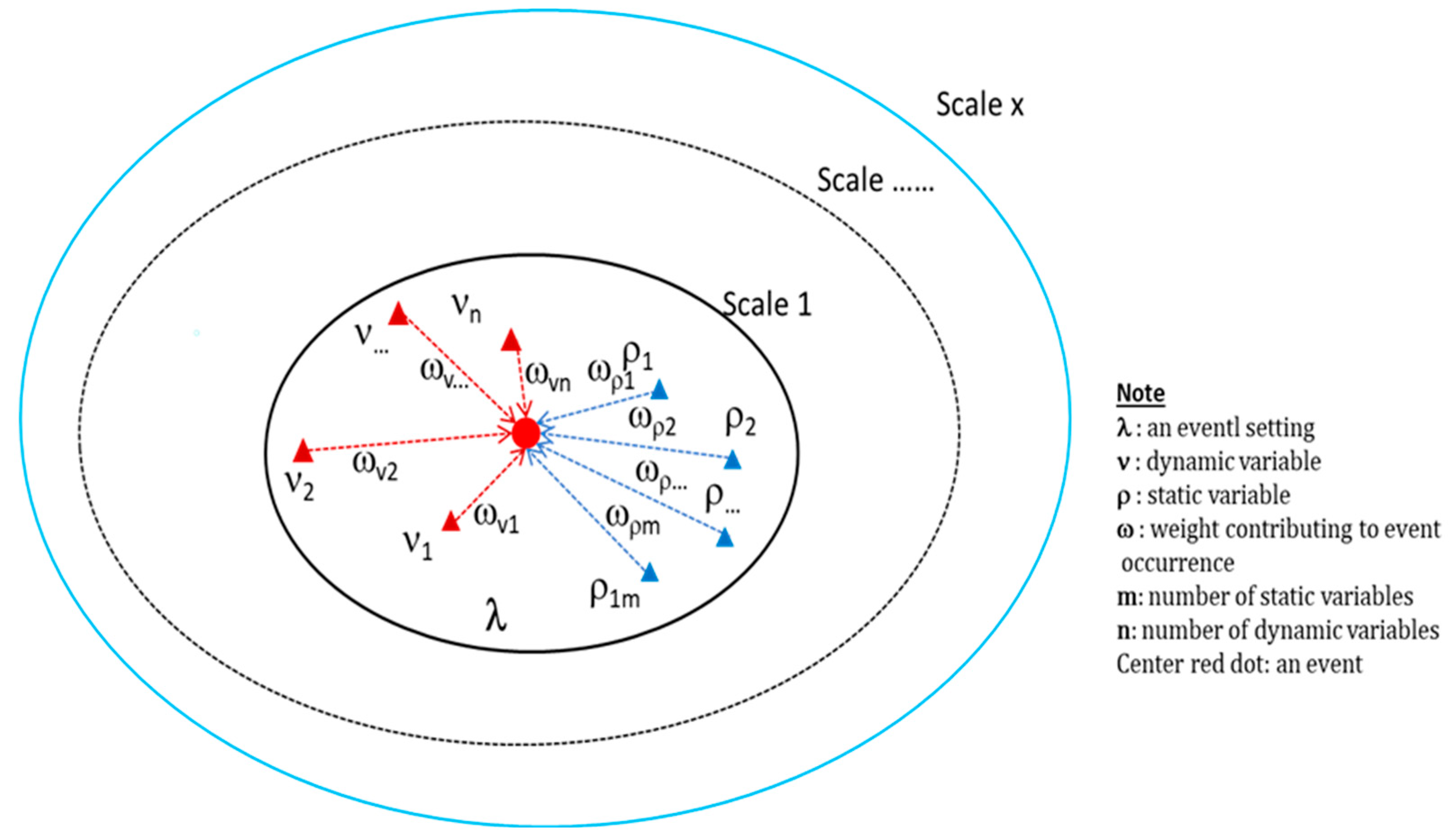
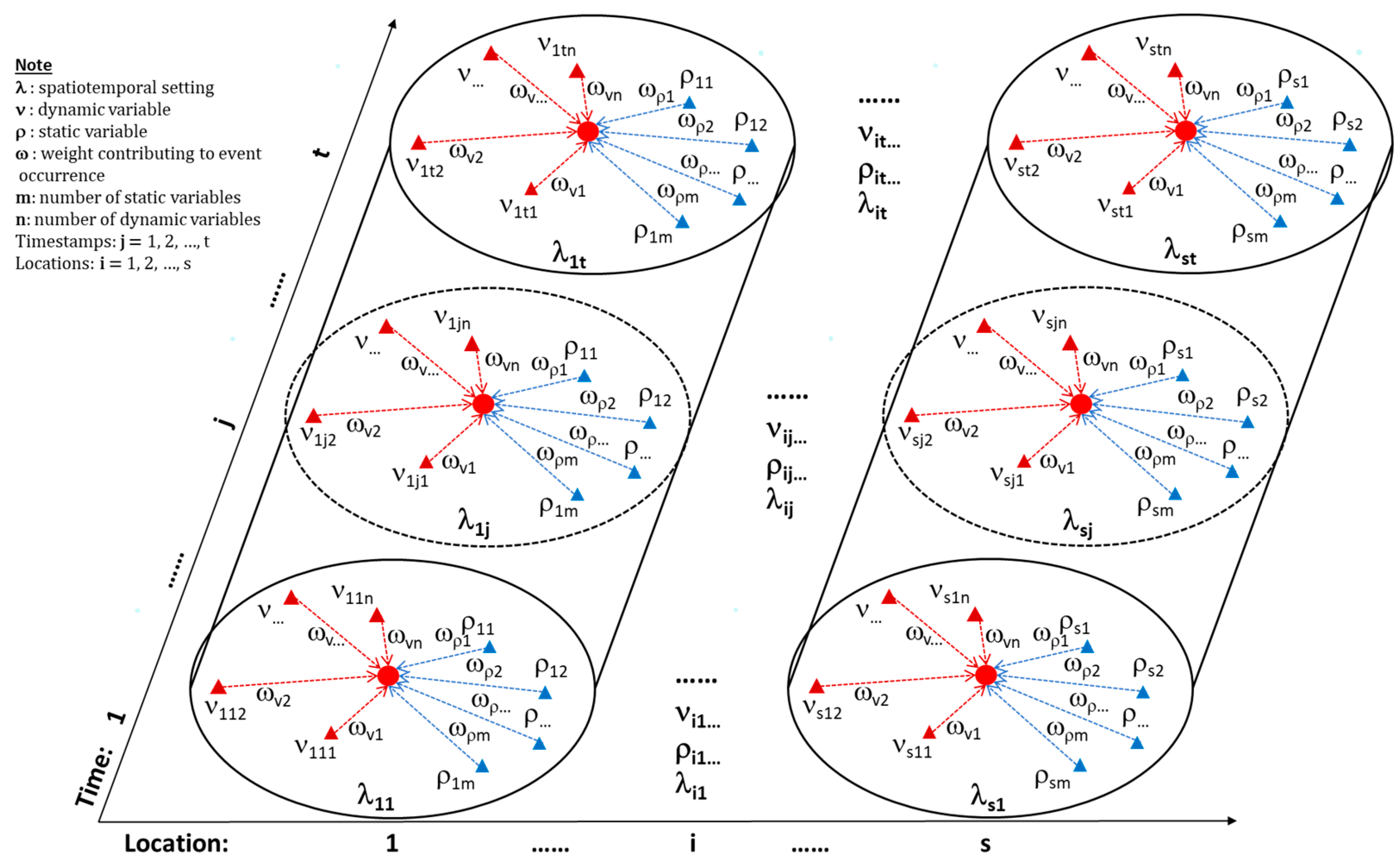
2.1. Model for Event Sequence Settings

As noted above, a conceptual challenge for modeling an event sequence setting lies in the spatial and temporal specification of the setting. The event sequence similarity measure described by Xu and Beard [1] assume time series and derived events sequences are observed at fixed point locations. Clearly, influences on a time series, and, by extension, a derived event sequence, extend beyond a point location, but a projected extent will be application and scale dependent, the scale dependence here being a function of pertinent event generating processes. As [12] note, the space of a site is something that emerges through unfolding event relations. Thus, we assume that the space of an event setting will vary based on the observed process, local environmental circumstances, and monitoring practices and have scale implications for variable selection.

As with most analyses, spatial and temporal scales must be considered in identifying and characterizing spatiotemporal event sequence settings. As a basis for modeling sequences of spatiotemporal event settings, we first model an event-situated setting at a specific temporal scale or time point with different spatial scales. Figure 1 illustrates the potential for different spatial boundaries for a setting. Where a boundary is placed has implications for the set of influencing factors. With changes in spatial scale, the influencing factors for a setting may vary and may be both static and dynamic.

To account for the dynamic aspects of setting as relating to an event sequence at a location, we conceptualize the setting as a sequence, i.e., a sequence of settings at ordered time points, as illustrated in Figure 2. The measurement of spatial pattern and heterogeneity is dependent on the scale at which the measurements are made. In this study, we do not consider interactions between scales. For a specific application context, we assume that we have determined the pertinent set of static and dynamic variables for representing all event settings at one spatial scale. For a set of monitored locations generating spatiotemporal event sequences as discussed in [1], we specify corresponding sequences of spatiotemporal event settings. Figure 2 graphically illustrates these conceptual sequences of spatiotemporal event settings with n dynamic and m static representative variables.

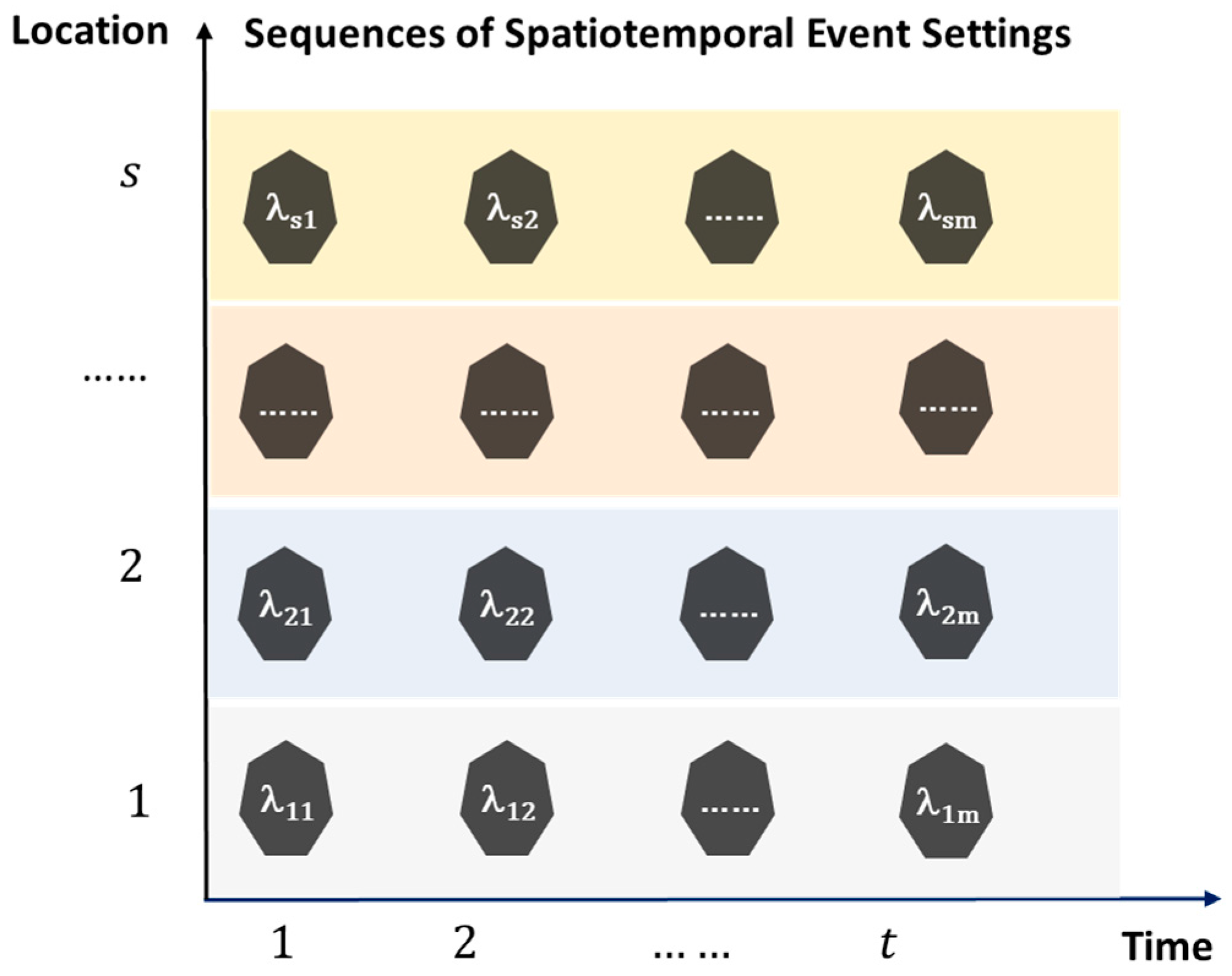
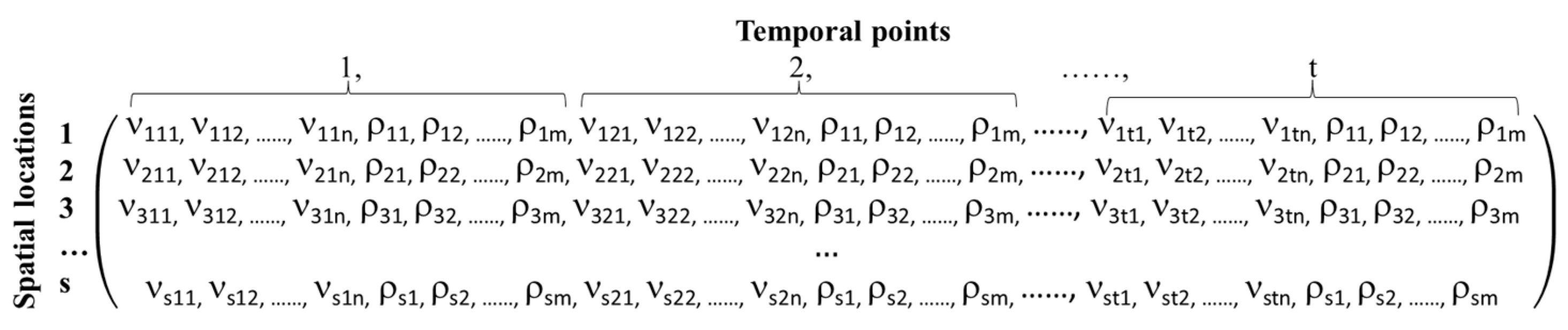
2.2. Matrix Representation of Sequences of Spatiotemporal Settings

For a given application context, we assume we have determined the major variables which strongly or satisfactorily represent the spatial settings for a set of sensor locations or monitoring stations where event sequences are observed. Given $s$ locations or monitoring stations and $t$ temporal points, we conceptually associate an event sequence with a setting sequence. We then represent these sequences of spatiotemporal event settings with a $s\times t$ matrix, as schematically illustrated in Figure 3.

For each setting $\mathsf{\lambda }$ with n dynamic (ν) and m static variables (ρ), i.e.,

$$\lambda :{\nu }_1,{\nu }_2,\dots \dots ,{\rho }_m,$$

Figure 3 can be expanded to Figure 4 to become the variables-based matrix representation of the sequences of spatiotemporal event settings.

2.3. Similarity Measures of Spatial Settings

2.3.1. Pairwise Similarity between Individual Spatial Settings

Pairwise similarity between individual settings is fundamental to further develop similarity measures between sequences of spatiotemporal settings based on certain criteria. In a study of environmental settings, for example, pairwise similarity can be used to measure the similarity between two or more settings based on factors such as temperature, humidity, rainfall, and other environmental variables. By calculating pairwise similarity scores, we can gain insights into how different or how similar settings relate to each other and identify patterns that may be useful in predicting future outcomes.

In this study, we develop a new pairwise similarity measure between spatial settings based on the modifications of the Jaccard index described in [1]. The original Jaccard index is a similarity measure commonly used in the context of sets or binary vectors, where each element can either be present or absent [39]. To adapt the Jaccard index for measuring the similarity between spatial settings associated with thematic events, we need to determine a set of common features, including static and dynamic variables, representing each spatial setting. Considering the number of common features for a pair of settings, we have two major considerations, (1) the magnitude or quantitative level of each element from both settings, and (2) that the values of the dynamic variables or elements should be measured at the same timestamps or time intervals.

We first identify the co-existing dynamic variables between two representative dynamic variable sets $l_{d1}$ and $l_{d2}$, and the co-existing static variables between two representative static variable sets $l_{s1}$ and $l_{s2}$ of two spatial settings, setting 1 and 2. We calculate the relative ratios of individual common variables, and then sum them by dynamic and static variables. The modified Jaccard similarity between two spatial settings at time k can be expressed as the sum of relative ratios of all common features/variables divided by the total number of unique features/variables in both sets/settings as in Equation (1):

Equation (1):

$$si{m}_k\left(l_1,l_2\right)=\frac{{Sd}_{k12}+{Ss}_{12}}{\left|l_{d1}\cup l_{d2}\right|+\left|l_{s1}\cup l_{s2}\right|}=\frac{{Sd}_{k12}+{Ss}_{12}}{N_d+N_s}$$

(1)

where

$l_1$—set 1 representing spatial setting 1, including the subset 1 of dynamic variables ($l_{d1}$) and the subset 2 of static variables $\left(l_{s1}\right)$,

$l_2$—set 2 representing spatial setting 2, including the subset 1 of dynamic variables ($l_{d2}$) and the subset 2 of static variables $\left(l_{s1}\right)$,

${Sd}_{k12}$—sum of relative ratios of common dynamic variables between two settings at time k,

${Ss}_{12}$—sum of relative ratios of common dynamic variables between two settings, assuming no changes over time during the experiment,

$N_d=\left|l_{d1}\cup l_{d2}\right|$—cardinality of union set of $l_{d1}$ and $l_{d2}$,

$N_s=\left|l_{s1}\cup l_{s2}\right|$—cardinality of union set of $l_{s1}$ and $l_{s2}$.

We have two similarity calculation situations dependent on variable types. First, if variable values are interval, ratio, binary and categorical, the pairwise similarity at time k can be calculated using Equations (2) and (3). Note that the categorical data can be converted to binary data format based on the number of categories.

If not considering weights or relative importance of individual elements/variables:

$$si{m}_k\left(l_1,l_2\right)=\frac{{\sum }_{i=1}^{Ckd12}\left(1-Abs\left(lev\left(d_{k1i}\right)-lev\left(d_{k2i}\right)\right)\right)+{\sum }_{j=1}^{Cs12}\left(1-Abs\left(lev\left(s_{1j}\right)-lev\left(s_{2j}\right)\right)\right)}{N_d+N_s}$$

(2)

If considering weights or relative importance of individual elements/variables:

$$si{m}_k\left(l_1,l_2\right)=\frac{c_{kd12}{\sum }_{i=1}^{Ckd12}{\omega }_i\left(1-Abs\left(lev\left(d_{k1i}\right)-lev\left(d_{k2i}\right)\right)\right)}{N_d}+\frac{c_{s12}{\sum }_{j=1}^{Cs12}{\omega }_j\left(1-Abs\left(lev\left(s_{1j}\right)-lev\left(s_{2j}\right)\right)\right)}{N_s}$$

(3)

Second, if variables are ordinal valued, the similarity can be calculated using Equations (4) and (5):

If not considering weights or relative importance of individual elements/variables:

$$si{m}_k\left(l_1,l_2\right)=\frac{{\sum }_{i=1}^{Ckd12}\left(1-\frac{Abs\left(lev\left(d_{k1i}\right)-lev\left(d_{k2i}\right)\right)}{n_i-1}\right)+{\sum }_{j=1}^{Cs12}\left(1-\frac{Abs\left(lev\left(s_{1i}\right)-lev\left(s_{2i}\right)\right)}{m_j-1}\right)}{N_d+N_s}$$

(4)

If considering weights or relative importance of individual elements/variables:

$$si{m}_k\left(l_1,l_2\right)=\frac{c_{kd12}{\sum }_{i=1}^{Ckd12}{\omega }_i\left(1-\frac{Abs\left(lev\left(d_{k1i}\right)-lev\left(d_{k2i}\right)\right)}{n_i-1}\right)}{N_d}+\frac{c_{s12}{\sum }_{j=1}^{Cs12}{\omega }_j\left(1-\frac{Abs\left(lev\left(s_{1i}\right)-lev\left(s_{2j}\right)\right)}{m_j-1}\right)}{N_s}$$

(5)

where

$c_{kd12}$—the number of common dynamic variables between two settings at timestamp k, $c_{s12}$—the number of common static variables between two settings,

${\omega }_i,{\omega }_j$—weights or relative importance of dynamic and static independent variables to response variable,

$n_i,m_j$—ordinal levels of dynamic variable i and static variable j, respectively,

$lev\left(d_{k1i}\right),lev\left(d_{k2i}\right)$—the relative levels or magnitudes of two corresponding co-occurring elements in two dynamic subsets $l_{d1}$ and $l_{d2}$ at timestamp k, respectively:

$$lev\left(d_{k1i}\right)=\frac{d_{k1i}}{d_{k1i}+d_{k2i}} \mathrm{and} lev\left(d_{k2i}\right)=\frac{d_{k2i}}{d_{k1i}+d_{k2i}}$$

(6)

${\omega }_i,{\omega }_j$—weights or relative importance of dynamic and static independent variables to response variable,

$lev\left(s_{1i}\right),lev\left(s_{2i}\right)$—the relative levels or magnitudes of two corresponding co-occurring elements in two static subsets $l_{s1}$ and $l_{s2}$, respectively:

$$lev\left(s_{1i}\right)=\frac{s_{1i}}{s_{1i}+s_{2i}} \mathrm{and} lev\left(s_{2i}\right)=\frac{s_{2i}}{s_{1i}+s_{2i}}$$

(7)

2.3.2. Pairwise Similarity between Sequences of Spatial Settings

Sequences of a spatial setting refer to the different configurations of the setting or a physical space that occur over time due to the changes of the dynamic variables while static variables are assumed stable during the study timeframe of interest. We can extend the modified Jaccard index-like pairwise similarity measure between individual settings, to calculate the pairwise similarity between sequences of spatial settings if the data from different locations are collected in equal time intervals or in the same order. Assuming we have determined the granularity of time intervals or certain sequential order and the total number of timestamps, T, the similarity between two sequences of spatial settings from two locations (S1 and S2) can be expressed as Equation (8):

$$\begin{gathered} si{m}_{global}\left(S_1,S_2\right)=\frac{{\sum }_{k=1}^{T}si{m}_k\left(l_1,l_2\right)}{T} \\ =\frac{{\sum }_{k=1}^T\left({Sd}_{k12}+{Ss}_{12}\right)}{T\left(N_d+N_s\right)} \\ =\frac{{\sum }_{k=1}^T{Sd}_{k12}}{T\left(N_d+N_s\right)}+\frac{{\sum }_{i=1}^T{Ss}_{12}}{T\left(N_d+N_s\right)} \\ =\frac{{\sum }_{k=1}^T{Sd}_{k12}}{T\left(N_d+N_s\right)}+\frac{{Ss}_{12}}{N_d+N_s} \end{gathered}$$

(8)

In dealing with the sequences of spatial settings, we also need to consider the data types and the weights or relative importance of explanatory variables to response variables (events or event sequences of interests). So, we also have four situations in which calculating the similarity between these setting sequences from different locations.

(1)

Variable type: interval, ratio, binary and categorical; not considering the weights of individual variables:

$$si{m}_{global}\left(S_1,S_2\right)=\frac{{\sum }_{k=1}^T{\sum }_{i=1}^{Ckd12}\left(1-Abs\left(lev\left({ld}_{k1i}\right)-lev\left({ld}_{k2i}\right)\right)\right)}{T\left(N_d+N_s\right)}+\frac{{\sum }_{j=1}^{Cs12}\left(1-Abs\left(lev\left({ls}_{1j}\right)-lev\left({ls}_{2j}\right)\right)\right)}{N_d+N_s}$$

(9)

(2)

Variable type: interval, ratio, binary and categorical; considering the weights of individual variables:

$$\begin{array}{ll}si{m}_{global}\left(S_1,S_2\right)=& \frac{c_{kd12}{\sum }_{k=1}^T{\sum }_{i=1}^{Ckd12}{\omega }_i\left(1-Abs\left(lev\left({ld}_{k1i}\right)-lev\left({ld}_{k2i}\right)\right)\right)}{N_d}\\ & +\frac{{T\ast c}_{s12}{\sum }_{j=1}^{Cs12}{\omega }_j\left(1-Abs\left(lev\left(s_{1j}\right)-lev\left(s_{2j}\right)\right)\right)}{N_s}\end{array}$$

(10)

(3)

Variable type: ordinal; not considering the weights of individual variables:

$$si{m}_{global}\left(S_1,S_2\right)=\frac{{\sum }_{k=1}^T{\sum }_{i=1}^{Ckd12}\left(1-\frac{Abs\left(lev\left(d_{k1i}\right)-lev\left(d_{k2i}\right)\right)}{n_i-1}\right)}{T\left(N_d+N_s\right)}+\frac{{\sum }_{j=1}^{Cs12}\left(1-\frac{Abs\left(lev\left(s_{1i}\right)-lev\left(s_{2i}\right)\right)}{m_j-1}\right)}{N_d+N_s}$$

(11)

(4)

Variable type: ordinal; considering the weights of individual variables:

$$\begin{array}{ll}si{m}_{global}\left(S_1,S_2\right)=& \frac{c_{kd12}{\sum }_{k=1}^T{\sum }_{i=1}^{Ckd12}{\omega }_i\left(1-\frac{Abs\left(lev\left(d_{k1i}\right)-lev\left(d_{k2i}\right)\right)}{n_i-1}\right)}{N_d}\\ & +\frac{{T\ast c}_{s12}{\sum }_{j=1}^{Cs12}{\omega }_j\left(1-\frac{Abs\left(lev\left(s_{1i}\right)-lev\left(s_{2i}\right)\right)}{m_j-1}\right)}{N_s}\end{array}$$

(12)

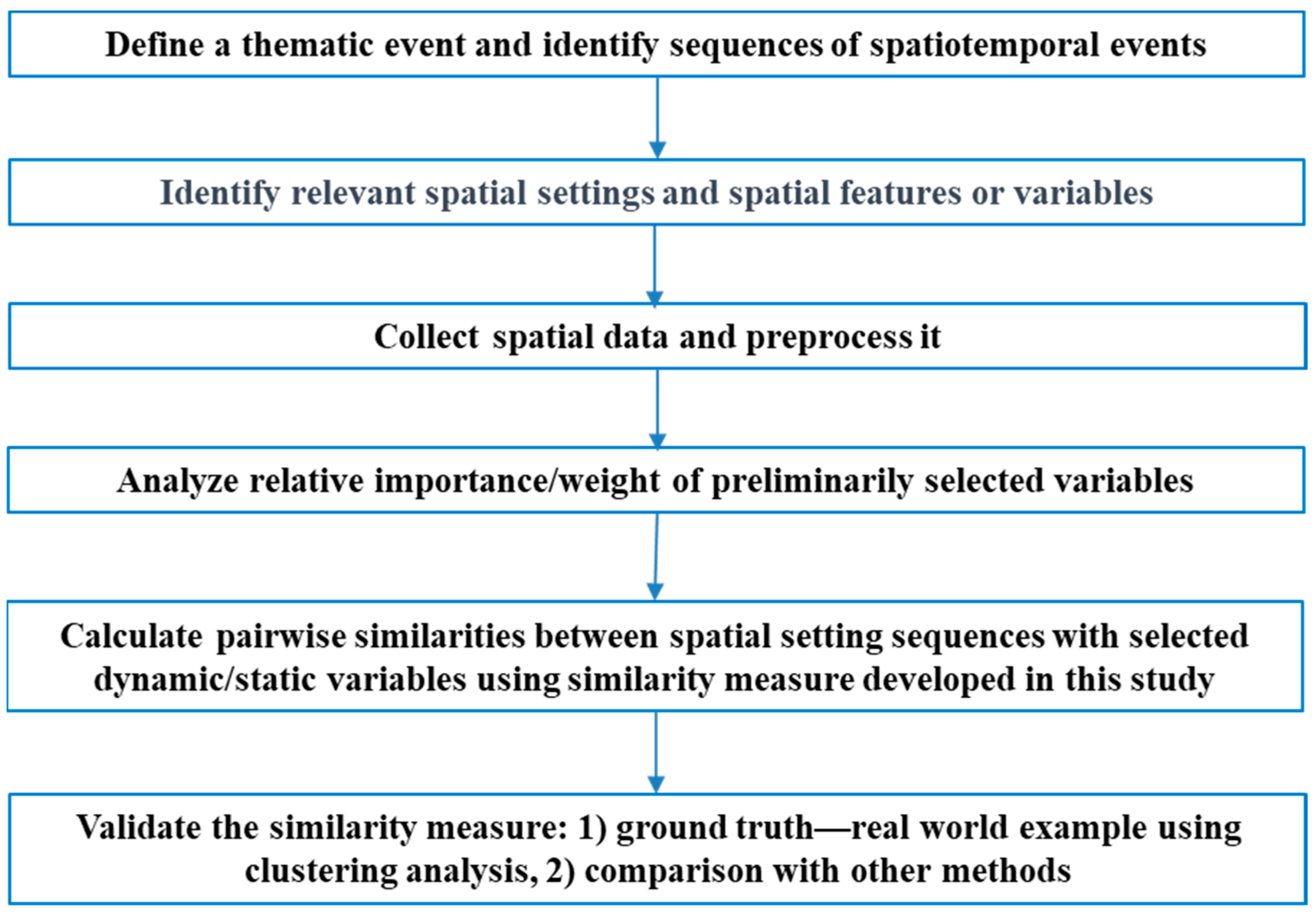
2.4. Setting Similarity Analysis Workflow

To estimate similarity levels between event settings, a critical step is to effectively select and quantify the major attributes representing these settings where events or event sequences occur. As introduced above, the variables can be static, dynamic, or both, potentially covering a wide range of environmental variables. The selection of variables in developing similarity measures will be domain dependent and should be statistically discriminant. In a water quality monitoring application, for example, the static spatial setting variables of interest could include land cover, topography, and soils, and dynamic variables could be weather related. Figure 5 shows the steps for implementing similarity assessment between event settings or sequences of event settings in a specific domain.

Define a thematic event and identify sequences of spatiotemporal events: assume that we focused on an event or event sequences related research in a specific domain and identified a series of sequences of spatiotemporal events and completed similarity analysis between these sequences.

Identify relevant spatial settings and spatial features or variables: select potential dynamic and static variables representing spatial settings, which are deemed relevant to event occurrences based on domain knowledge. In studying air pollution events, for example, we could include data on such variables as wind direction, wind speed, sites of local manufactures, major pollution sources, concentration of major pollutants, and transportation density. A correlation matrix for these initial selected variables can be used to eliminate redundant information.

Collect spatial data and preprocess it: collect sufficient data on pre-selected static and dynamic variables intuitively correlated to occurrences of thematic events. Preprocessing or preparation of the collected data mainly includes normal distribution check, normalization, standardization of measurement units, and binarization of categorical data.

Analyze relative importance/weight of preliminarily selected variables: to improve the computation speed and accurate representation of similarity measures we should identify those variables most relevant to the events of interest and reduce the number. To determine which variables are most important to the thematic events and for the similarity measures, we can conduct relative weight analysis (RWA) [40,41,42] and partial least squares regression (PLSR) [43].

Calculate pairwise similarities between spatial setting sequences: Once the most relevant features or variables are identified, we can use the similarity measures developed in this study to compute the pairwise similarity between spatial settings and sequences of spatial-temporal settings and form the similarity matrix.

Validate the similarity measure: with the similarity matrix of spatial setting sequences, we can further conduct clustering analysis to group event sequences associated with locations or stations, and then conduct the comparison analysis with clusters of event sequences as ground truth. The other approach is to compare the results with other methods.

3. Case study: Setting Similarity of Coastal Monitoring Stations for Fecal Pollution

To demonstrate the use of our proposed method above, we determined the pairwise similarities of 16 monitoring stations along the Maine coast with the selected setting attributes for costal fecal pollution event sequences. The Maine Department of Marine Resources (DMR) manages the shellfish growing areas in coastal Maine based on the fecal pollution situations observed from more than 2000 monitoring stations. Fecal coliform is a type of bacteria that is found in the intestines and feces of warm-blooded animals, including humans. It is used as an indicator of fecal contamination of water [44]. Monitoring fecal coliform levels in coastal waters is important because it can help identify sources of contamination and provide an early warning of contamination, enabling faster responses. Maine DMR typically collects water samples at these monitoring stations (>2000) at regular intervals and analyzes them for fecal coliform levels. Grouping monitoring stations as similar spatial settings of fecal pollution events can provide several benefits and advantages. First, it can provide useful information for early detection of pollution events at similar stations [45,46]. Second, cluster analysis of monitoring stations across a wider area can help to identify trends and patterns in fecal coliform levels and pollution events, which can inform efforts to improve water quality. Third, followed by the previous two benefits, it will help to optimize resource allocation and prioritize monitoring efforts based on areas of higher pollution risk, which can help to reduce costs and increase efficiency in monitoring and management activities. Fourth, it can help to make more informed decisions about pollution control measures, such as beach closures or water treatment. Lastly, it also helps to increase public awareness of coastal water quality issues and the need for responsible use and management of marine resources.

3.1. Experimental Site and Design

3.1.1. Site and Variables

In this case study, we selected 16 monitoring stations along the Maine coast, with the following DMR assigned location IDs: WE020.00, WE028.00, WG008.10, WG027.00, WG038.00, WM003.00, WN057.00, WN077.20, WQ023.00, WR011.00, WS027.00, WS051.00, WT015.00, WT018.00, WT024.00, WV019.00, as shown on the map (Figure 6). Multiple factors related to fecal coliform concentration around these monitoring stations contribute to characterizing the corresponding spatial settings for fecal pollution events. Some studies have shown that shoreline, basin hydrology, and marine environment affect the retention, survival, and distribution of fecal coliform [47]. Based on data availability, we selected a combination of basin characteristics as static variables and some marine environmental factors as dynamic variables. Their abbreviations and description are shown in

Table 1. Description and abbreviation of selected basin characteristics and dynamic parameters.

Abbreviation/Code	Description	Unit
Static Variables	(Basin Characteristics)
BSLDEM10M	Mean basin slope computed from 10 m DEM	percent
COASTDIST	Shortest distance from the coastline to the basin centroid	miles
DRNAREA	Area that drains to a point on a stream	square miles
ELEV	Mean Basin Elevation	feet
ELEVMAX	Maximum basin elevation	feet
LC11DEV	Percentage of developed (urban) land from NLCD 2011 classes 21–24	percent
LC11IMP	Average percentage of impervious area determined from NLCD 2011 impervious dataset	percent
PCTSNDGRV	Percentage of land surface underlain by sand and gravel deposits	percent
SANDGRAVAF	Fraction of land surface underlain by sand and gravel aquifers	dimensionless
SANDGRAVAP	Percentage of land surface underlain by sand and gravel aquifers	percent
STATSGOA	Percentage of area of Hydrologic Soil Type A from STATSGO	percent
STORAGE	Percentage of area of storage (lakes ponds reservoirs wetlands)	percent
STORNWI	Percentage of storage (combined water bodies and wetlands) from the National Wetlands Inventory	percent
BKSF	Bank-full Streamflow	ft^3/s
BKW	Bank-full Width	ft
BKD	Bank-full Depth	ft
BKA	Bank-full Area	ft^2
Pop_Dnsity	Population Density	persons/mi^2
Dynamic Variables
Tide	Tide stages: H, L, F, E, HF, HE, LF, LE	3 h
Salinity	Ocean water salinity
Wind	Wind direction: E, S, W, N, NW, NE, SW, SE	Direction
RainCum24	Cumulative precipitation in 24 h	inch
RainCum48	Cumulative precipitation in 48 h	inch
RainCum72	Cumulative precipitation in 72 h	inch
RainCum96	Cumulative precipitation in 96 h	inch

.

3.1.2. Data Collection

We used the geolocations of the 16 selected monitoring stations to delineate the corresponding basins with StreamStats v4.13.0 (https://streamstats.usgs.gov/ss/, the access date: 25 February 2023) and download all associated basin characteristics data. For the static variables described in Table 1, the data were extracted as shown in Table S1. We obtained marine environment related variables and fecal coliform measurements from Maine DMR (Table S2).

3.1.3. Methods

We used partial least squares regression (PLSR) analysis [41,42] to obtain the relative importance of all variables against the fecal coliform scores. We used the similarity measure developed in this study to achieve the similarity matrix of spatial setting sequences, and used the method developed in [1] to obtain the similarity matrix of the corresponding fecal pollution event sequences with the same locked timestamps. After converting the similarity matrices of both setting and event sequences to the distance matrices, we performed a cluster analysis [48].

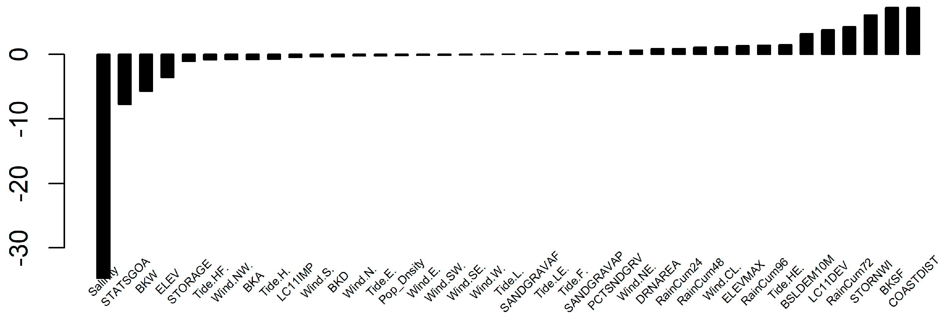
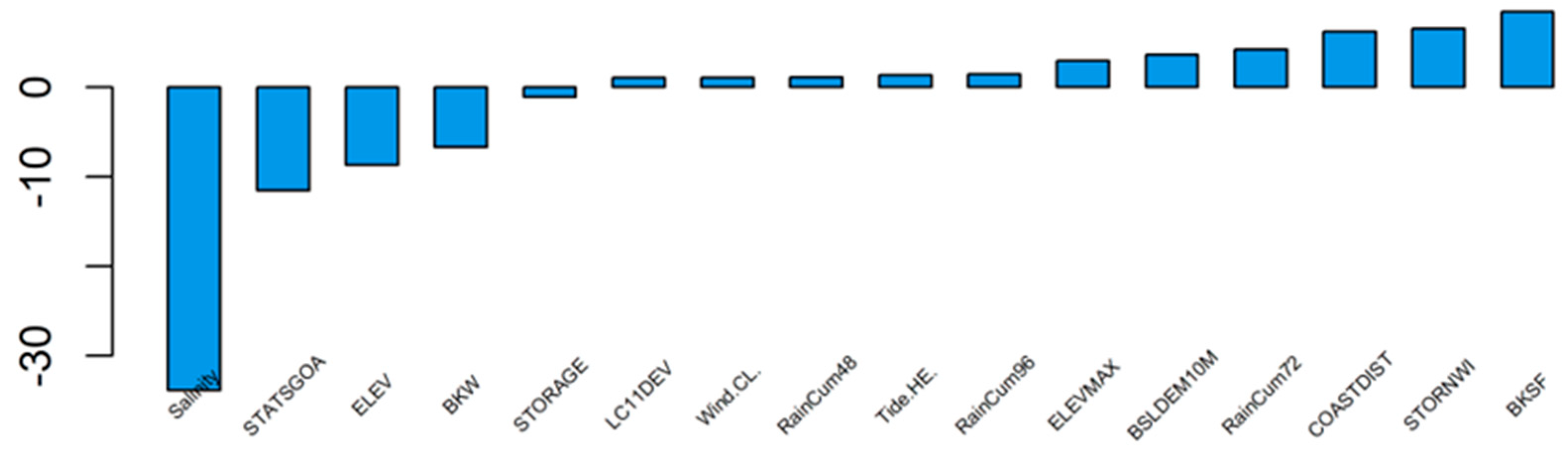
3.2. Relative Weights and Selection of Representative Variables for Spatial Settings

The results of the partial least squares regression analysis on 39 variables revealed that some variables are more important than others in predicting the fecal coliform levels (

Table 2. Relative weights of 39 selected variables with signs.

Negative Variables	Relative Importance	Positive Variables	Relative Importance
Salinity	−34.696	COASTDIST	7.252
STATSGOA	−7.763	BKSF	7.217
BKW	−5.725	STORNWI	6.092
ELEV	−3.630	RainCum72	4.256
STORAGE	−1.069	LC11DEV	3.789
Tide.HF.	−0.817	BSLDEM10M	3.200
Wind.NW.	−0.790	Tide.HE.	1.455
BKA	−0.778	RainCum96	1.389
Tide.H.	−0.771	ELEVMAX	1.298
LC11IMP	−0.472	Wind.CL.	1.121
Wind.S.	−0.373	RainCum48	1.082
BKD	−0.372	RainCum24	0.878
Wind.N.	−0.247	DRNAREA	0.871
Tide.E.	−0.218	Wind.NE.	0.654
Pop_Dnsity	−0.186	PCTSNDGRV	0.399
Wind.E.	−0.109	SANDGRAVAP	0.393
Wind.SW.	−0.106	Tide.F.	0.325
Wind.SE.	−0.095	Tide.LE.	0.042
Wind.W.	−0.056	SANDGRAVAF	0.004
Tide.L.	−0.015

and Figure 7). The signs associated with each variable provide insight into the direction of their impact on the fecal coliform levels. Salinity has the highest relative importance and the strongest negative influence on the fecal coliform. On the other hand, shortest distance from the coastline to the basin centroid (COASTDIST), bank-full streamflow (BKSF), and percentage of storage (combined water bodies and wetlands) from the National Wetlands Inventory (STORNWI) have the highest positive influence on the fecal coliform levels.

To reduce the number of variables for calculating similarity in the formula developed in this study, we selected the variables with higher weights. In this case study, we selected those variables with absolute values of relative importance greater than 1. We then re-ran PLSR with these selected variables against corresponding fecal coliform levels. The relative importance of these variables from the second round PLSR is shown in

Table 3. Relative weights of 16 selected variables with signs.

Negative Variables	Relative Importance	Positive Variables	Relative Importance
Salinity	−33.900	BKSF	8.500
STATSGOA	−11.500	STORNWI	6.500
ELEV	−8.700	COASTDIST	6.200
BKW	−6.700	RainCum72	4.200
STORAGE	−1.100	BSLDEM10M	3.700
		ELEVMAX	3.000
		Tide.HE.	1.400
		RainCum96	1.400
		LC11DEV	1.100
		Wind.CL.	1.100
		RainCum48	1.100

and Figure 8, which can be used as relative weights for calculating similarities between spatial setting sequences when considering contribution from these individual variables.

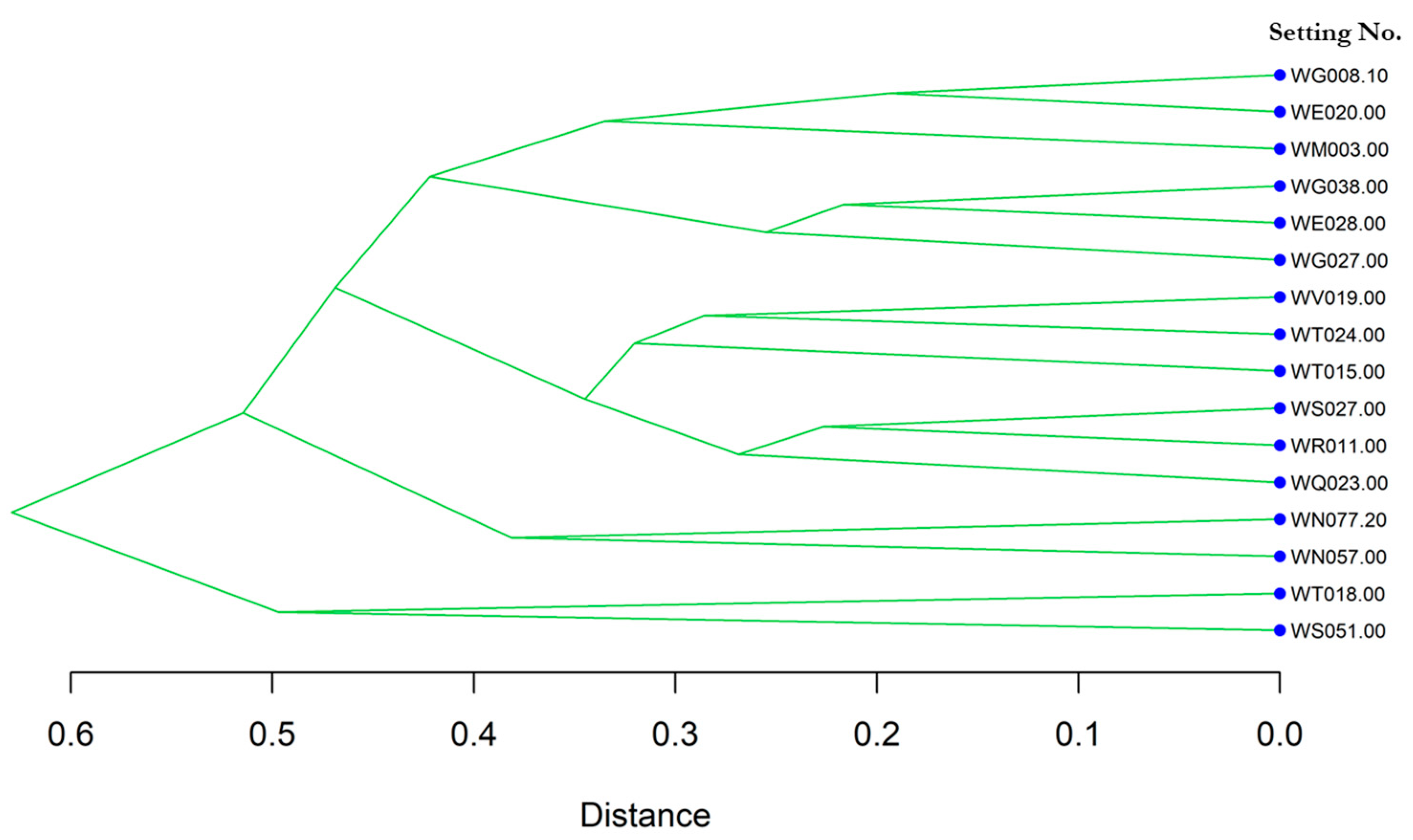
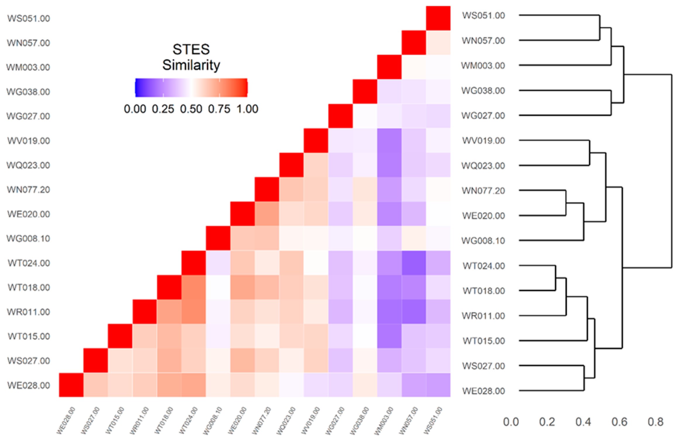
3.3. Clustering Analysis of Spatial Setting Sequences and Fecal Pollution Event Sequences

We computed all pairwise similarities between spatial setting sequences using the method of this study using the 16 selected variables in the previous section for 16 rain-storm-involved timestamps. The clustering analysis of spatial setting sequences labeled with monitoring stations yields interesting insights into the underlying patterns and structures of the data of these selected static and dynamic variables (Figure 9). The result indicates that there are 3~4 distinct clusters within the data, with each cluster representing a unique pattern of spatial setting sequences with similar characteristics. Figure 9 shows some geographically proximate spatial setting sequences in the same or connected clusters, but not all due to the diverse contributions of different static and dynamic variables. These clusters provide valuable information about the types of spatial setting sequences, which we next relate to clusters of fecal pollution event sequences.

We generated a similarity matrix between fecal pollution event sequences also labeled with monitoring stations and the corresponding setting sequences at the same time frame (16 days). With the conversion to the distance matrix, we implemented the clustering analysis and the similarity heatmap, and the clustering result is shown in Figure 10. Three major clusters are clearly identified.

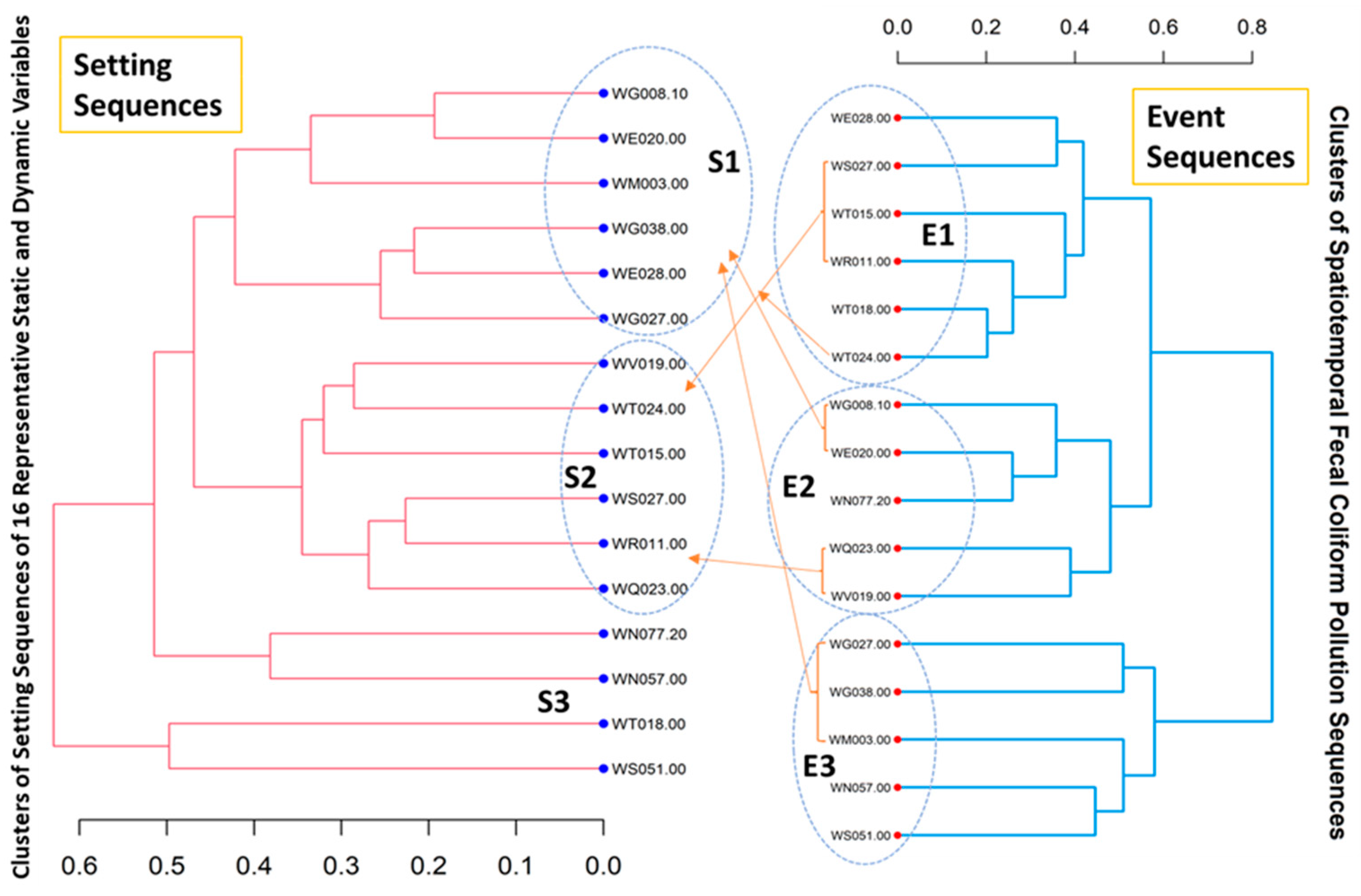
3.4. Cross Analysis between Clusters of Setting Sequences and Clusters of Event Sequences

Cross-analysis between clusters of spatial settings and clusters of events sequences can provide insights into the causes and effects of pollution events in coastal waters. We put the clustering results above from both setting sequences and event sequences side by side to build the cross-comparison graph (Figure 11). By examining components of the major clusters of setting sequences and pollution event sequences, we find cases of at least two stations within one major cluster among the event sequence clusters that were also grouped in the same major cluster of setting sequence clusters. We found 11 out of 16 monitoring stations showing this pattern. Specifically, WS027.00, WT015.00, WT024.00, and WR011.00 in event sequence Cluster E1 are also in setting sequence Cluster S2; WG008.10 and WE020.00 in Cluster E2 are also in Cluster S1; WQ023.00 and WV019.00 in Cluster E2 are also in Cluster S2; and WG027.00, WG038.00, and WM003.00 in Cluster E3 are also in Cluster S1. This cross-analysis between clusters of spatial settings and event sequences can help to improve our understanding of the complex interactions between environmental factors and basin characteristics and identify drivers for fecal coliform pollution events in coastal marine water.

4. Discussion

We developed similarity measures through modeling spatial setting sequences. The model uses a matrix representation of spatiotemporal event settings and considers both static and dynamic variables. To measure the similarity between spatial settings, the Jaccard index is modified based on the variables’ magnitude and the time interval at which dynamic variables are measured. Pairwise similarity between individual spatial settings is crucial for developing similarity measures between sequences of spatiotemporal settings based on specific criteria. The pairwise similarity measure can help to identify patterns and predict future outcomes of corresponding event sequences.

The model’s matrix representation of sequences of spatiotemporal settings can be used to represent a set of sensor locations or monitoring stations where event sequences are observed. The matrix representation has the flexibility to include n dynamic and m static variables that represent all event settings at one spatial scale. The modified Jaccard index measures the similarity between individual spatial settings and forms the basis for similarity measures between sequences of spatiotemporal settings. The modified Jaccard similarity between two spatial setting sequences considers the relative ratios of common features/variables. These measures provide information on the differences or similarity of spatial settings, which in turn contribute to the analysis of event sequences arising from these settings.

Through the case study, we demonstrated how to model the spatial-temporal setting sequences and provide a useful framework for understanding and characterizing spatial setting sequences corresponding to event sequences. The model’s focus on defining the bounds of a setting and considering both static and dynamic variables allows for a comprehensive understanding of associated event sequences. The pairwise similarity measure helps identify patterns in event settings or setting sequences to comprehensively understand better the occurrences of events and event sequences. The similarity measures developed in this paper, and the framework incorporating static and dynamic variables to represent settings, will provide useful tools for a range of applications, from environmental settings to predictive modeling.

One potential application of similarity measures for event sequence settings is in the field of disaster management. By analyzing the spatial-temporal settings of past disasters, emergency responders can better predict the likelihood and potential impact of future disasters and allocate resources more effectively. For example, if a particular region is prone to frequent flooding, similarity measures can be used to identify patterns in the spatial-temporal settings of past floods and help emergency responders anticipate and prepare for future floods in that region. [49] studied the relationship between hydrological similarity measures and regional flooding frequency. The authors studied the similarity measures between catchments in the distribution of rainfall extremes and the extent of the impervious portion of the catchment. Similarly, our setting sequence similarity measures could be used to compare the frequency distribution of rainfall extremes and the extent of imperviousness across catchments. This could help identify catchments that have similar characteristics in terms of their rainfall and land use and may also be suitable for pooling together in regional flooding frequency analysis. [50] found that land cover/land use change (LCLUC) and sediment runoff affected by forestry practices and livestock grazing is temporally related to the water quality. We can potentially extend our similarity measures to this study to compare the temporal patterns of land disturbance and water quality variables (total suspended solids (TSS), turbidity, and visual clarity). This could help identify whether changes in land disturbance are related to changes in water quality over time, and whether there are any spatial relationships between land disturbance and water quality. In addition, as mentioned in this research, there exist nonlinear changes in land disturbance and sediment runoff; our novel approach on similarity between setting sequences can be easily plugged in to study these nonlinear ecosystem dynamics.

Overall, the use of similarity measures for event setting sequences has a wide range of potential applications in various fields, including disaster management, urban planning, transportation planning, and cultural heritage management. By analyzing the spatiotemporal context of events and their surrounding environmental factors, researchers and practitioners can gain a deeper understanding of the underlying mechanisms that drive those corresponding events and event sequences and use that knowledge to make more informed decisions about the management and planning of future events and activities.

5. Conclusions

In conclusion, modeling spatiotemporal event sequences requires careful consideration of spatial and temporal scales to define the bounds of the setting. The dynamic aspects of the setting should also be accounted for by conceptualizing the setting as a sequence. A matrix representation of sequences of spatiotemporal event settings can be developed for each setting with both dynamic and static variables. Pairwise similarity between individual settings and sequences of spatial settings can be calculated based on modifications of the Jaccard index, using a set of spatial features that represent each spatial setting.

With a careful consideration of spatial and temporal scales to define the bounds of the setting, we developed a modeling approach that incorporates dynamic variables or features in addition to static variables. Using a matrix-based representation of spatiotemporal setting sequences, we developed new similarity measures that include quantitative levels of individual elements within the sequence and comparison with locked timestamps or order. These similarity measures allow for the use of all variable data types in the equations. Overall, these similarity measures, along with the matrix-based representation of spatiotemporal event setting sequences incorporating both static and dynamic variables, provide a novel method in support of event sequence analysis.

Future research could investigate the potential of using the proposed similarity measures to analyze the dynamics of complex systems, such as ecological or economic systems, where events and their settings or contexts can be critical factors in understanding the system behavior. By examining the similarity of event settings, researchers could gain insight into how different factors interact with each other over time and across different spatial scales, which could inform better decision-making in a wide range of fields, from urban planning to disaster management.

References

1. Xu, F.; Beard, K. A Unifying Framework for Analysis of Spatial-Temporal Event Sequence Similarity and Its Applications. ISPRS Int. J. Geo-Inf. 2021, 10, 594. [Google Scholar] [CrossRef]
2. Lupiani, E.; Sauer, C.; Roth-Berghofer, T.; Juarez, J.M.; Palma, J. Implementation of similarity measures for event sequences in myCBR. In Proceedings of the 18th UKCBR Workshop, Cambridge, UK, 10 December 2012. [Google Scholar]
3. Guralnik, V.; Srivastava, J. Event detection from time series data. In Proceedings of the fifth ACM SIGKDD International Conference on Knowledge Discovery and Data Mining, San Diego, CA, USA, 1 August 1999; pp. 33–42. [Google Scholar]
4. Moen, P. Attribute, Event Sequence, and Event Type Similarity Notions for Data Mining. Ph.D. Thesis, University of Helsinki, Helsinki, Finland, 2000. [Google Scholar]
5. Mannila, H.; Ronkainen, P. Similarity of event sequences. In Temporal Representation and Reasoning, Proceedings of the Fourth International Workshop; IEEE Computer Society Press: Washington, DC, USA, 1997; pp. 136–139. [Google Scholar]
6. Obweger, H.; Suntinger, M.; Schiefer, J.; Raidl, G. Similarity searching in sequences of complex events. In the 2010 Fourth IEEE International Conference on Research Challenges in Information Science; Springer: Berlin/Heidelberg, Germany, 2010; pp. 631–640. [Google Scholar]
7. Wongsuphasawat, K.; Plaisant, C.; Taieb-Maimon, M.; Shneiderman, B. Querying event sequences by exact match or similarity search: Design and empirical evaluation. Interact. Comput. 2012, 24, 55–68. [Google Scholar] [CrossRef]
8. Simandan, D. Being surprised and surprising ourselves: A geography of personal and social change. Prog. Hum. Geogr. 2020, 44, 99–118. [Google Scholar] [CrossRef]
9. Paasi, A. Place and region: Looking through the prism of scale. Prog. Hum. Geogr. 2004, 28, 536–546. [Google Scholar] [CrossRef]
10. Malpas, J. Putting space in place: Philosophical topography and relational geography. Environ. Plan D Soc. Space 2012, 30, 226–242. [Google Scholar] [CrossRef]
11. Schatzki, T.R. The Site of the Social: A Philosophical Account of the Constitution of Social Life and Change; Penn State University Press: University Park, PA, USA, 2002. [Google Scholar]
12. Marston, S.A.; Jones, J.P., III; Woodward, K. Human geography without scale. Trans. Inst. Br. Geogr. 2005, 30, 416–432. [Google Scholar] [CrossRef]
13. Woodward, K.; Jones, J.P., III; Marston, S.A. The politics of autonomous space. Prog. Hum. Geogr. 2012, 36, 204–224. [Google Scholar] [CrossRef]
14. Worboys, M.; Hornsby, K. From objects to events: GEM, the geospatial event model. In Proceedings of the International Conference on Geographic Information Science, Adelphi, MD, USA, 20–23 October 2004; pp. 327–343. [Google Scholar]
15. Moore, A. Rethinking scale as a geographical category: From analysis to practice. Prog. Hum. Geogr. 2008, 32, 203–225. [Google Scholar] [CrossRef]
16. Jiang, B.; Yao, X. Location based services and GIS in perspective. In Location Based Services and Telecartography; Springer: Berlin/Heidelberg, Germany, 2007; pp. 27–45. [Google Scholar]
17. Dey, A.K. Understanding and using context. Pers. Ubiquitous Comput. 2001, 5, 4–7. [Google Scholar] [CrossRef]
18. Brézillon, P.; Gonzalez, A.J. Context in Computing: A Cross-Disciplinary Approach for Modeling the Real World; Springer: Berlin/Heidelberg, Germany, 2014. [Google Scholar]
19. Loke, S. Context-Aware Pervasive Systems: Architectures for a New Breed of Applications; CRC Press: Boca Raton, FL, USA, 2006. [Google Scholar]
20. Zolnik, E.J. Context in human geography: A multilevel approach to study human–environment interactions. Prof. Geogr. 2009, 61, 336–349. [Google Scholar] [CrossRef]
21. Sunley, P. Context in economic geography: The relevance of pragmatism. Prog. Hum. Geogr. 1996, 20, 338–355. [Google Scholar] [CrossRef]
22. Weber, J.; Kwan, M.-P. Evaluating the effects of geographic contexts on individual accessibility: A multilevel Approach1. Urban Geogr. 2003, 24, 647–671. [Google Scholar] [CrossRef]
23. Gong, H.; Hassink, R. Context sensitivity and economic-geographic (re) theorising. Camb. J. Reg. Econ. Soc. 2020, 13, 475–490. [Google Scholar] [CrossRef]
24. Simandan, D. Revisiting positionality and the thesis of situated knowledge. Dialogues Hum. Geogr. 2019, 9, 129–149. [Google Scholar] [CrossRef]
25. Delbosc, A.; Currie, G. The spatial context of transport disadvantage, social exclusion and well-being. J. Transp. Geogr. 2011, 19, 1130–1137. [Google Scholar] [CrossRef]
26. Timmermans, H.; van der Waerden, P.; Alves, M.; Polak, J.; Ellis, S.; Harvey, A.S.; Kurose, S.; Zandee, R. Spatial context and the complexity of daily travel patterns: An international comparison. J. Transp. Geogr. 2003, 11, 37–46. [Google Scholar] [CrossRef]
27. Cutter, S.L. Vulnerability to environmental hazards. Prog. Hum. Geogr. 1996, 20, 529–539. [Google Scholar] [CrossRef]
28. Roux, A.V.D.; Mair, C. Neighborhoods and health. Ann. N. Y. Acad. Sci. 2010, 1186, 125–145. [Google Scholar] [CrossRef]
29. Sampson, R.J. The neighborhood context of well-being. Perspect. Biol. Med. 2003, 46, S53–S64. [Google Scholar] [CrossRef]
30. Yang, D.-H.; Goerge, R.; Mullner, R. Comparing GIS-based methods of measuring spatial accessibility to health services. J. Med. Syst. 2006, 30, 23–32. [Google Scholar] [CrossRef]
31. Wolpert, J. The decision process in spatial context. Ann. Assoc. Am. Geogr. 1964, 54, 537–558. [Google Scholar] [CrossRef]
32. Gripenberg, S.; Roslin, T. Up or down in space? Uniting the bottom-up versus top-down paradigm and spatial ecology. Oikos 2007, 116, 181–188. [Google Scholar] [CrossRef]
33. Tilman, D.; Kareiva, P. Spatial Ecology: The Role of Space in Population Dynamics and Interspecific Interactions (MPB-30); Princeton University Press: Princeton, NJ, USA, 2018; Volume 30. [Google Scholar]
34. Singhal, A.; Luo, J.; Zhu, W. Probabilistic spatial context models for scene content understanding. In the Computer Vision and Pattern Recognition, 2003, Proceedings of the 2003 IEEE Computer Society Conference; IEEE: Piscataway, NJ, USA, 2003; p. I. [Google Scholar]
35. Heitz, G.; Koller, D. Learning spatial context: Using stuff to find things. In Proceedings of the European Conference on Computer Vision, Munich, Germany, 8–14 September 2008; pp. 30–43. [Google Scholar]
36. Keßler, C. Similarity measurement in context. In Proceedings of the International and Interdisciplinary Conference on Modeling and Using Context, Roskilde, Denmark, 20–24 August 2007; pp. 277–290. [Google Scholar]
37. Keßler, C.; Raubal, M.; Janowicz, K. The effect of context on semantic similarity measurement. In Proceedings of the OTM Confederated International Conferences “On the Move to Meaningful Internet Systems”, Rhodes, Greece, 21–25 October 2007; pp. 1274–1284. [Google Scholar]
38. Levin, S.A. The problem of pattern and scale in ecology: The Robert H. MacArthur award lecture. Ecology 1992, 73, 1943–1967. [Google Scholar] [CrossRef]
39. Choi, S.-S.; Cha, S.-H.; Tappert, C.C. A survey of binary similarity and distance measures. J. Syst. Cybern. Inform. 2010, 8, 43–48. [Google Scholar]
40. Chao, Y.-C.E.; Zhao, Y.; Kupper, L.L.; Nylander-French, L.A. Quantifying the relative importance of predictors in multiple linear regression analyses for public health studies. J. Occup. Environ. Hyg. 2008, 5, 519–529. [Google Scholar] [CrossRef] [PubMed]
41. Tonidandel, S.; LeBreton, J.M. RWA web: A free, comprehensive, web-based, and user-friendly tool for relative weight analyses. J. Bus. Psychol. 2015, 30, 207–216. [Google Scholar] [CrossRef]
42. Tonidandel, S.; LeBreton, J.M.; Johnson, J.W. Determining the statistical significance of relative weights. Psychol. Methods 2009, 14, 387. [Google Scholar] [CrossRef]
43. Ali, F.; Rasoolimanesh, S.M.; Sarstedt, M.; Ringle, C.M.; Ryu, K. An assessment of the use of partial least squares structural equation modeling (PLS-SEM) in hospitality research. Int. J. Contemp. Hosp. Manag. 2018, 30, 514–538. [Google Scholar] [CrossRef]
44. Noble, R.T.; Moore, D.F.; Leecaster, M.K.; McGee, C.D.; Weisberg, S.B. Comparison of total coliform, fecal coliform, and enterococcus bacterial indicator response for ocean recreational water quality testing. Water Res. 2003, 37, 1637–1643. [Google Scholar] [CrossRef]
45. Dong, J.; Wang, G.; Yan, H.; Xu, J.; Zhang, X. A survey of smart water quality monitoring system. Environ. Sci. Pollut. Res. 2015, 22, 4893–4906. [Google Scholar] [CrossRef] [PubMed]
46. Prasad, A.; Mamun, K.A.; Islam, F.; Haqva, H. Smart water quality monitoring system. In Proceedings of the 2015 2nd Asia-Pacific World Congress on Computer Science and Engineering (APWC on CSE), Nadi, Fiji, 2–4 December 2015; pp. 1–6. [Google Scholar]
47. Hughes, K.A. Influence of seasonal environmental variables on the distribution of presumptive fecal coliforms around an Antarctic research station. Appl. Environ. Microbiol. 2003, 69, 4884–4891. [Google Scholar] [CrossRef] [PubMed]
48. Kettenring, J.R. The practice of cluster analysis. J. Classif. 2006, 23, 3–30. [Google Scholar] [CrossRef]
49. Castellarin, A.; Burn, D.; Brath, A. Assessing the effectiveness of hydrological similarity measures for flood frequency analysis. J. Hydrol. 2001, 241, 270–285. [Google Scholar] [CrossRef]
50. Kamarinas, I.; Julian, J.P.; Hughes, A.O.; Owsley, B.C.; De Beurs, K.M. Nonlinear changes in land cover and sediment runoff in a New Zealand catchment dominated by plantation forestry and livestock grazing. Water 2016, 8, 436. [Google Scholar] [CrossRef]
Figure 1. Schematic representation of an event-situated setting considering different spatial scales for the setting. Influencing factors with different weights are shown only at Scale 1. More, fewer, or different sets of factors may apply at another scale.
Geographies 03 00016 g001
Figure 2. Schematic illustration of sequences of spatial-temporal settings with t time points and s locations.
Geographies 03 00016 g002
Figure 3. Schematic matrix representation of sequences of spatial-temporal settings with t time points and s locations.  λ st—a setting at location s and time t.
Geographies 03 00016 g003
Figure 4. Matrix representation of sequences of spatiotemporal event settings with s locations and t time points.
Geographies 03 00016 g004
Figure 5. Spatial-temporal setting similarity analysis flowchart.
Geographies 03 00016 g005
Figure 6. Selected monitoring stations/locations on the Maine coast for depicting spatiotemporal settings of fecal pollution event sequences.
Geographies 03 00016 g006
Figure 7. Bar chart of relative importance of 39 selected static and dynamic explanatory variables for fecal coliform bacterial measurements.
Geographies 03 00016 g007
Figure 8. Bar chart of relative importance of 16 selected static and dynamic variables against fecal coliform bacterial measurements.
Geographies 03 00016 g008
Figure 9. Clusters of 16 spatial setting sequences labeled with monitoring stations.
Geographies 03 00016 g009
Figure 10. Similarity-based heat map and distance based hierarchical clustering between 16 monitoring stations for fecal pollution event sequences.
Geographies 03 00016 g010
Figure 11. Cross analysis between clusters of setting sequences and clusters of event sequences.
Geographies 03 00016 g011