Article

Comparison of Earthquake and Moisture Effects on Rockfall-Runouts Using 3D Models and Orthorectified Aerial Photos

by
Mohammad Al-Shaar
1,*,
Pierre-Charles Gérard
1,
Ghaleb Faour
2,
Walid Al-Shaar
1,* and
Jocelyne Adjizian-Gérard
1
1
Geography Department, CREEMO (Centre de Recherche en Environnement-Espace Méditerranée Orientale), Saint-Joseph University, Campus des Sciences Humaines, Rue de Damas, Mar Mikhael, Beirut 1104 2020, Lebanon
2
National Center for Remote Sensing, National Council for Scientific Research (CNRS), Beirut 1107 2260, Lebanon
*
Authors to whom correspondence should be addressed.
Geographies 2023, 3(1), 110-129; https://doi.org/10.3390/geographies3010006
Submission received: 19 November 2022 / Revised: 7 January 2023 / Accepted: 12 January 2023 / Published: 16 January 2023
(This article belongs to the Special Issue Advanced Technologies in Spatial Data Collection and Analysis)

Abstract

:
Rockfall hazard gains popularity nowadays among researchers in different scientific fields, decision-makers and urban planners. The assessment of rockfall hazard requires detection, mapping and estimating the maximum travel distance that rock boulders may reach, commonly known as “rockfall runout”. This latter can change significantly under the effects of different triggering factors such as soil conditions, chemical, physical and geological rock properties. However, comparing and analyzing these different effects represents, to the best of our knowledge, one of the newest scientific challenges that need to be addressed. This paper presents a complete methodologic approach aiming to assess the rockfall hazard through runout estimation in three different conditions: (i) gravity, (ii) earthquakes, and (iii) the presence of moisture along the slope. The “Mtein” Village and its surrounding areas in the Mount Lebanon region were chosen as the study area because there have been numerous historic rockfalls and various-sized rocks, such as cobbles and boulders, scattered throughout the area. Thus, three-dimensional simulations were conducted using the Rockyfor3D software and aerial photos for the year 1999 to assess the rockfall runout, the energy curves, and the number of deposited rocks. The results reveal that earthquakes have the highest triggering effect on rockfall and that moisture has a damping effect on RFs by decreasing the kinetic energy. The study shows the importance of taking into consideration the influence of triggering factors as well as rock density on rockfall runout and hazard.

1. Introduction

Rockfalls (RFs) are considered a devastating type of mass movement event because of the fast motion and the high kinetic energy carried by the rock when it usually falls from high elevations with steep slopes [1]. Due to the fast development of urbanization in mountainous areas, where steep slopes and unstable rocks exist, the risk of RF hazard increases within these newly developed areas [2]. Accordingly, because of the complexity and the numerous factors affecting RF, many studies have developed different and dissimilar methodologies to assess the RF hazard and identify the different causing factors and their effects. The majority of methods used for RF hazard/risk assessment are divided into two main types: quantitative and qualitative. The quantitative approach depends on numerical values such as the numerical probability and frequency of detachment, including propagation and intensity [3]. On the other hand, the qualitative method is based on descriptive terms such as ranked attributes, weighted indices, rating systems, scoring schemes, ranking matrices and classifications. The results are expressed using relative terms such as high, medium and low [3,4,5]. Generally, it was found in different studies that elevations, slopes and rock materials play an important role in increasing or decreasing the fast movement of the rock [6,7,8,9].
These factors are not considered the main causing factors. However, the RF action takes place when rocks lose their stability when a triggering factor (e.g., dynamic fractures in steep slopes, rainfall, seismic activity, gravity coupled with the instability of rock blocks, vegetation and human activities) gives unexpected energy, pushing the rock blocks to slide, topple, or fall from a sub-vertical surface that is considered the source area [10,11]. The impact consumes limited energy but lets the block continue its way by bouncing and flying along curvy trajectories or rolling on talus and debris slopes. Following that, first ground impact, elevations, slopes and rock sizes could be considered secondary causing factors. Previous studies have quantified the RF runout aspects in terms of rock velocities and runouts. For instance, many studies have quantified the aforementioned aspect by taking into consideration the earthquake [12,13,14,15] and the moisture content [16] as triggering factors. These studies investigated earthquakes and moisture content as triggering factors of RFs; nonetheless, a comparative analysis showing the difference in rockfall runout distances and the possible number of rocks deposited was not conducted. In addition, and to the best of the authors’ knowledge, investigating the effects of different factors on RFs with the existence of different lithologies was not previously conducted. Examining and taking into account the effects of lithology is considered a key factor for RFs modeling since it can induce substantial changes in modeling results [9,17]. This paper contributes to this growing literature by investigating and discussing the effects of RF-triggering factors. In a more detailed way, this research develops a methodology to assess and compare the effect sizes of two main triggering factors: earthquake and moisture. This methodology could be applied later on, for further studies, in an extended form to compare the effects of other driving factors. In a more detailed way, the study aims to show and compare the effects of earthquakes and moisture on the kinetic energy of falling rocks and on the deposited number of blocks in the study area. For this purpose, three simulations were conducted. The case of gravity-induced RFs was considered the baseline for the comparison of simulation results for earthquake and moisture scenarios. High-resolution historical aerial photos for the selected study area taken in 1999 were used as the main input data for the simulations of runout modeling in addition to other types of information. More details on data collection and processing are elaborated in the Section 2. The study area is located in the western part of the Mount Lebanon area. It was selected since: (i) numerous historic RFs happened and different-sized rocks, such as cobbles and boulders, are scattered all over the area; and also (ii) since the changes in some triggering factors could be observed. More details are presented in the study area section. With respect to the technological tools used to conduct the runout modeling simulations and with the recent evolution of technology, many computer programs were developed to simulate RF runout, these computer platforms can perform either: (i) 2D analysis such as the Colorado Rockfall Simulation Program—CRSP [18], and RocFall® [19]; or (ii) 3D analysis such as the STONE by [20], Rockyfor3D [7], Rocpro3D© [21], and RAMMS© rockfall [22]. A study conducted by [12] showed that the 3D RF simulation software was able to better present the actual trajectories and led to more accurate and consistent results than 2D simulation and analysis. Therefore, the 3D simulations will be conducted on the platform of the Rockyfor3D software. Additional details of the simulations are presented in the modeling approach section. The block sizes range from small cobbles to large boulders of hundreds or even thousands of cubic meters in volume, and could move at speeds from a few meters to tens of meters per second. Therefore, places exposed and vulnerable to this hazard form a threat to people, buildings and utilities when this natural hazard takes place [3,23,24]. In this context, the study of RF runout modeling is very important for hazard and risk mitigation plans, especially when comparing the effect sizes of the triggering factors. The RF runout modeling techniques would: (i) predict the dynamic movement of a fallen block along a slope; (ii) calculate the energy carried at any point of its trajectory; and (iii) give out the probability of reaching a point located at a distance from the source area.
These outcomes would give useful information on areas prone to RF hazard and good indications of the triggering factors. This information could be used as guidance in order to direct decisions towards potential effective methods to be adopted to mitigate the risk. In addition, this study presents a full technique to assess the RF hazard in the absence of RF records and inventory. The study also highlights the value of historical aerial photos in RF hazard and risk assessment. It is hypothesized that earthquakes have an effect on increasing the initial kinetic energy as well as the kinetic energy during the rock-falling stage for limestone and sandstone rocks. Previous studies, such as that conducted by Zheng et al. (2022) [25], examined the effect of earthquakes on kinetic energy without taking the lithology of the rocks into consideration. Moreover, it is assumed that an earthquake will increase the deposited number of RFs.
In addition, it is also hypothesized that higher moisture content in soil and rock has a damping, as decreasing, effect on RFs velocity after rock impact with the soil, known as a “bouncing” movement. Previous studies, such as that conducted by Vick et al. (2019) [16], indicated that high water content in soil materials would slow down the RFs of volcanic rocks that follow a bouncing movement. These studies did not take into consideration the effects of rock water content on RFs or the effects of soil moisture on RFs for sandstone and limestone rocks.
These two hypotheses are tested in this paper for validation. This research is limited to the study of only limestone and sandstone sedimentary rocks, which represent the lithology types of all rocks in the study area.
This paper is structured as follows: Section 2 presents the case study and highlights the methodology of the research and the techniques of data collection. In addition, it presents the rockfall modeling framework. Section 3 reveals and discusses, respectively, the obtained results. Section 4 summarizes the paper and discusses the future areas of relevant research.

2. Materials and Methods

2.1. Selection of the Study Area

The area of interest in our study is located in the western part of Mount Lebanon (Figure 1), 35 km away from the capital of Lebanon: Beirut. The “Mtein” Village and its surrounding areas in the Mount Lebanon region were selected as the study area since numerous historic rockfalls happened and different-sized rocks such as cobbles and boulders are scattered all over the area. The elevations range between 900 and 1200 m, with an average value of 1100 m (Saint Joseph University, 2021). In more detail, four historical aerial photos were taken in 1999 (scale, 1:10,000; camera focal length: 153.401 mm) were orthorectified with ERDAS Imagine software and used for this research. These photos cover an area of 12.7 square kilometers (km2), representing 0.12% of the total area of Lebanon. This region includes parts of five main villages: Mtein, Mchikha, Bzebdine, Hasabaya El Matn and Qaaqour. This specific zone was selected based on the fact that many RFs were detected and observed through aerial photo interpretation and during multiple field visits, respectively.
The lengths of the majority of RFs slopes observed in the study area are considered medium and range between 250 m and 350 m in distance.
Additionally, this area is characterized by a high mean annual rainfall range. For instance, the annual mean rainfall in Mtein ranges between 1200 and more than 1400 mm [26]. The geological aspects of the study area are extracted from a geological map (scale, 1:50,000) prepared by Michel Majdalani (BTD) and based on the geological map of Dubertert [27].

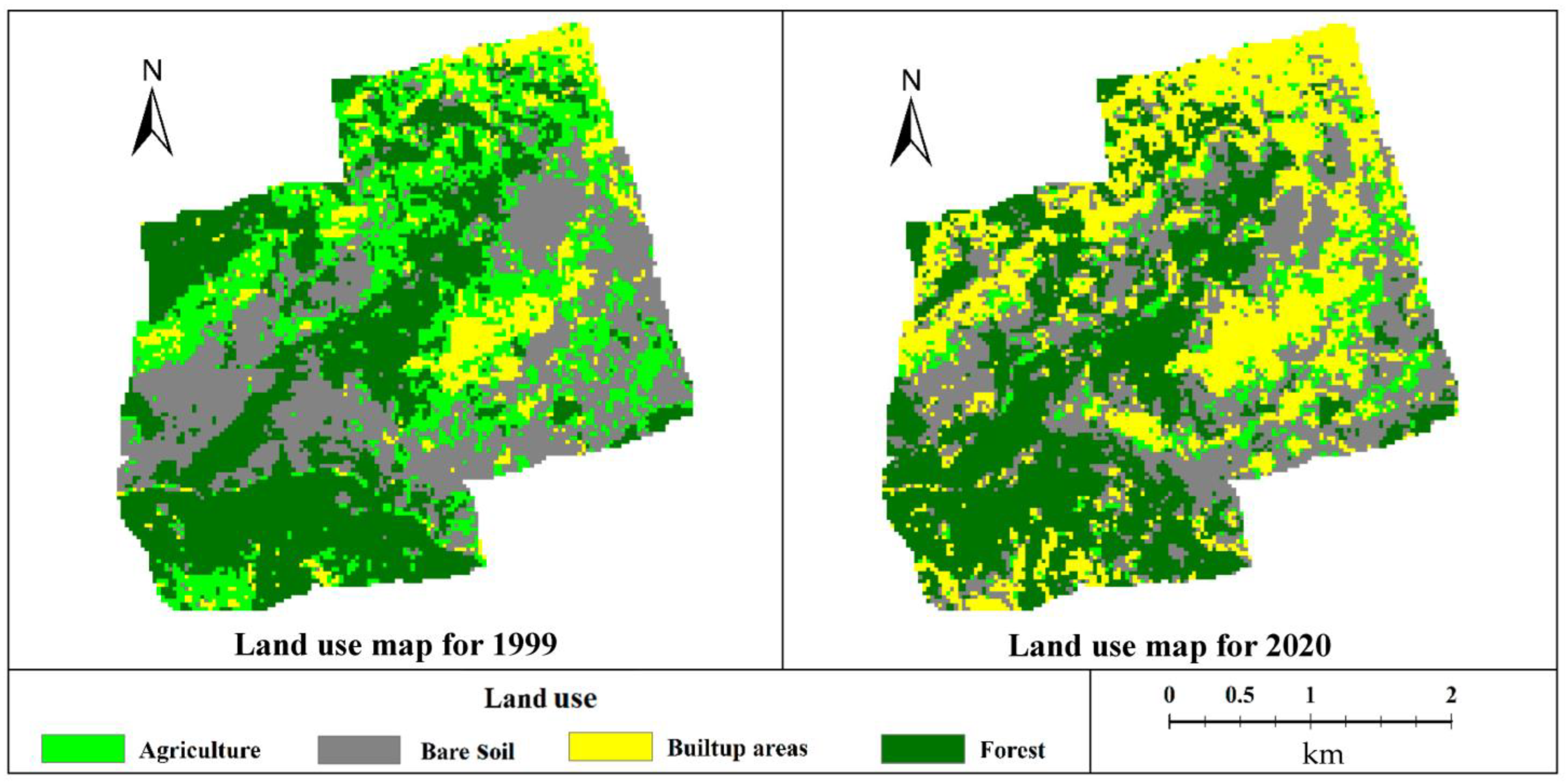
2.2. Urban Development: Land Use Classification

Moreover, two land use maps of 30 m resolution were generated in ArcMap software using the Landsat satellite images (Earthexplorer, 2021) in order to estimate the urban expansion, as new built-up areas, between the years 1999 and 2020, as shown in Figure 2. Therefore. Two Landsat satellite images of the study area for the years 1999 (Landsat 7, 2 level 2) and 2020 (Landsat 8, 2 level 2), with 30 m resolution, were extracted from the website of (Earthexplorer, 2021) to be then employed for the land use classification process.
It is noteworthy that Landsat level 2 images are atmospherically corrected (Earthexplorer, 2020). The supervised maximum likelihood classification method was adopted for the generation of two land use maps for the years 1999 and 2020. The purpose of generating the land use maps is to delimit the built-up areas and show the rate of urbanization, specifically under the RF risks, in the study area. The land use maps showed that the built-up areas have increased by 23.52% during this short period of time, with almost no awareness about the RF hazard where several buildings observed were built on or just under the source area of RFs (Figure 3 and Figure 4). The accuracy assessment tests for the land use classifications were conducted by computing the confusion matrices in ArcGIS software. The accuracy percentages for the land use maps of the years 1999 and 2020 were equal to 88% and 85%, respectively. Similarly, the corresponding kappa values for the years 1999 and 2020 are equal to 0.83 and 0.8, respectively. These values reveal a strong accuracy for the classification processes [28,29]. This test was conducted by creating 100 randomly distributed points over the classified land use map. The land use map classes in these points were compared to ground truth extracted by using an ESRI satellite image as a base map. In the context of this unprotected urban development, rockfall mapping is necessary to identify areas prone to RFs risks.

2.3. Rockfall Mapping Techniques

The literature indicated different data acquisition techniques that were used to produce rockfall maps. For instance, remote sensing and in situ investigation techniques were proposed for the purpose of mapping RF runouts and estimating their rocks’ volumes. These methods are classified as: (1) airborne, such as Unmanned Aerial Vehicles (UAVs) [30], airplane imagery [31] and airborne LiDAR [32]; (2) satellite imagery, such as very high-resolution images (VHR) from satellite sensors, multispectral and hyperspectral sensors [33]; and (3) ground-based: photogrammetry such as High Dynamic Range (HDR) [34] and terrestrial laser scanning techniques such as terrestrial LiDAR [32]. In the context of these RF mapping practices, the use of high-resolution historical aerial photos provides valuable information, especially when combined with present data. These photos would lead to a better comprehension of the complex RF mechanism and its evolution over a period of time (tens of years, for instance). In addition, historical aerial photos allow us to obtain: (a) qualitative information when interpreted as feature surface identification [31]; and (b) quantitative data when properly ortho-rectified, so they can be used for taking measurements.

2.4. Research Methodology and Materials

The methodology consists of conducting and comparing the results of three scenarios of 3D simulations for the RF runout models. The objective is depicted as assessing and comparing the effects of the earthquake and moisture with reference to the gravity-induced RFs case. The methodological approach is divided into four stages: (i) collection of data; (ii) data processing; (iii) runout model simulations; and (iv) comparative analysis. The collected data were processed through a sequence of several steps. The following section presents a detailed explanation of data collection and the corresponding processes. The developed methodology is presented graphically in Figure 5.

2.4.1. Aerial Photos and Interpretation

A series of four aerial photos, taken in the year 1999 by the Directorate of Geographic Affairs (Lebanese army, Ministry of Defense), was used for photo interpretation in the study area. Thus, four historical aerial photos are first interpreted to locate the entire RFs distribution area, including the release areas. They are then corrected geometrically using the orthorectification technique in ERDAS Imagine software to transform them into base maps. The four ortho-rectified base maps were merged into one base map using the image mosaic module in ERDAS Imagine software. Afterwards, the RFs’ locations were indicated on this base map, including the size of each rock boulder seen and measured on the field during the site visits conducted in June and July 2021.
The interpretation process was based on the stereo-pairing technique for these photos using a stereoscope. This technique allows the detection of major historic RF events and the acquisition of qualitative information, including the source area of RF (release area), the main scarp, the slope, and the accumulation zone where different-sized rock boulders are distributed. In a more detailed way, aerial photo interpretation is a helpful technique that could be used to investigate slope stability and identify landslides based on geomorphological features [35]. In view of that, the set of high-resolution historical aerial photos was used in this study as the base data for the adopted methodology. This type of data was used in this study as the sole source of information since Lebanon does not have a published landslide inventory map [36], and consequently, no RF inventory exists for the study area. In addition, the aerial photos were used to derive quantitative information with good accuracy, such as landslide extent and metric model [31]. To overcome the matter of photo distortions, the aerial photos were corrected by the ortho-rectification technique, which allows the acquisition of a map with correct distances.

2.4.2. Orthorectification

Using analytical photogrammetry, aerial photos are adjusted by removing photo distortions in order to create orthophotos (photos with true distances). The idea of orthorectification is to establish a correlation between the coordinates of photo points (image coordinates) and the real ground coordinates. This technique can be used when multiple inputs are available, usually derived from the calibration report of the camera that took the photos. For the photos used in this research, there was no calibration report; however, the needed parameters are indicated in the upper strip part of the photograph.
Rocchini et al. (2012) [37] have detailed a method of orthorectification. The procedure is divided into four steps: (1) collection of the main input parameters (digital elevation model, fiducial marks coordinates, focal length, principal point coordinates and ground control points); (2) interior orientation; (3) exterior orientation; and (4) rectification and resampling. For this purpose, the input parameters are collected as follows: (a) 5 m digital elevation model (DEM); (b) 8 fiducial marks coordinates were determined using the open tool, ImageJ software [38]; (c) the principal point is assumed to be the center of the image coordinate system, so the value 0 is assigned to the X and Y coordinates of this point; (d) the focal length was written on the upper strip part of the photo; and (e) 18 to 20 ground control points were collected for each photo using GPS during field visits, the points were located at the corners of the building, since these points are fixed and yield more accuracy for the process, in addition, the points are well distributed all over each of the used photos to enhance the quality of the orthophoto. The technique is computerized using ERDAS Imagine software, the interior orientation is done graphically by manually marking the fiducial marks to relate the image coordinate to the photo coordinate system (camera sensor). The exterior orientation was also done by marking the corresponding points on the scanned aerial photo after entering the ground control point coordinates, including X, Y and their elevation Z, into the software. The parameters collected and computed in the above steps are used to rectify each aerial image; all images are then resampled with the nearest neighbor assignment.
The validation indicator used was the root-mean-square error (RMSE). The guidelines provided by the National Standard for Spatial Data Accuracy (NSSDA) [39] indicated a value of 2.5 m as the maximum allowable RMSE value to validate the ortho rectification of a map with a scale of 1:10,000. In this context, the RMSE values for the four aerial photos were under the value 1.8, which shows the accuracy of the orthorectification process for these photos.

2.4.3. Mapping Rockfalls Distribution

Mapping the locations and volumes of fallen blocks is a very important process for risk investigation, as indicated by past studies that employed measurements and estimations of the block’s number and respective volumes [40,41]. Therefore, the RFs sizes have been measured in the field using a measuring tape where locations are accessible. Nevertheless, some of the boulders are not reachable. For this reason, their lengths and widths have been visually estimated and compared to the corresponding dimensions provided by the aerial photos. This comparison asserted the validity of the aforementioned estimation process with a maximal difference of ±0.3 m Furthermore, the height of the inaccessible boulders was visually estimated through field observation, in which the height of the inaccessible rockfalls was compared to nearby well-known height objects, such as buildings or boulders with measured heights.
In addition, six field visits were conducted between the months of June and July 2021 in order to inspect the lithology and size of RF boulders and examine soil types and the obstacles along the slope profile. A measuring tape was used to measure the dimensions of RFs boulders in accessible areas and a handheld GPS was used to mark the coordinates of RFs blocks. The lithology was determined by checking the physical characteristics, such as color, texture, and grain size, of the visible outcrops of the release areas and rock boulders. Some rock boulders are not accessible on the site, so they were photographed and compared to nearby rock blocks that were accessible. Then, the dimensions were estimated using the orthorectified aerial photos. The soil type was examined in the field by hand. The water was added to the soil sample and rolled in hand to determine the composition and texture. For instance, if the sample feels sticky in the hand, it would be clay material. Otherwise, it is typically sand [42]. The data obtained from the field examinations were compatible with those provided and validated by the soil type map prepared by the National Council for Scientific Research (NCSR)-Lebanon [43].
A geological map was used to determine and validate the types of rocks distributed all over the study area. The geological map was prepared by Michel Majdalani (BTD) and based on the geological map of Dubertert [27]. It is used to determine the rock lithology in the release areas in order to generate the rock density map in QGIS. Similarly, the soil map of Lebanon prepared by the NCSR-Lebanon (scale 1:50,000) [43] was employed to define the soil types. The rock density and soil maps are rasterized and then converted to ASCII raster file format in QGIS as input for the simulations in a later stage.
In line with the geological formation of rocks, the area of interest is dominated by limestone and sandstone rocks and encompasses the rock formations as follows: (A) Late Jurassic formations (J4–J7), thick-bedded to massive, highly fractured, jointed and well-karstified limestones and dolomitic limestone rocks: (1) J4-Liassic to Kimmeridgian (Kesrouane limestone formation) comprising limestone and dolomite rock types; (2) J5-Lower Portlandian (Bhannes formation) constituted of fine-grained Marls and Marly limestones and basalt intrusions; (3) J6-Upper Portlandian (Bikfaya formation) made of limestone and dolomitic limestone rocks; (4) J7-Upper Portlandian (Salima Formation), detritic limestone rocks; and (B) Lower Cretaceous formation: C1-Neocomian-Barremian (Chouf Grès de base) containing quartzitic and calcareous sandstones with intercalations of siltstone and clays.
Accordingly, the rock locations, type and densities, as well as the soil types, were determined.
According to the aforementioned processes, the RF map was produced in ArcGIS software. Consequently, a total of 209 rock boulders were mapped on the orthophotos in order to examine the RFs’ size distribution. This map, as illustrated in Figure 6, shows, according to the aerial photo interpretation and the field observations: (i) the past falling blocks and their volume sizes ranging from 0.7 to 2284 cubic meters; (ii) the source area of RFs (the release area); and (iii) the maximum traveled distance by the fallen rocks.

2.4.4. Digital Elevation Model

A contour topographic map (elevation interval: 5 m; scale: 1:20,000) provided by the Directorate of Geographic Affairs of the Lebanese army (Saint-Joseph University, 2021) was used to derive a digital elevation model (DEM) of 5-m resolution based on the interpolation process of ArcMap Software. This DEM was used in the simulation and the photo orthorectification processes.

2.4.5. Runout Simulations

The runout simulations are based mainly on the geometry and material properties of the rock fragments as well as the slope [44]. For instance, several parameters that are required to create a runout simulation are summarized in the following [18]: (1) slope inclination and length (slope profile); (2) surface roughness; (3) coefficients of restitution: normal and tangential; and (4) size and type/density of rocks. The produced RF map and the created DEM, in addition to rock and soil aspects, were inserted as inputs to run the simulations in Rockyfor3D (Version 5.2.15) software.
Rockyfor3D is a commercial 3D modeling software (not open source) that is used to create 3D models/simulations of rockfalls. The model used is probabilistic and process-based. The simulations in this software require the input data of a digital elevation model (DEM) along with other input parameters: (a) rock densities for rockfall sources; (b) dimensions of the blocks (height, width and length) and also the shape of the blocks; (c) slope surface roughness; (d) normal coefficient of restitution (nCOR) which is directly linked to the soil type existing on the slope; and (e) tangential coefficient of restitution (tCOR). The parameters needed for the simulation were collected from the data of the aforementioned maps (RFs distribution map, DEM, geological and soil maps) and from the conducted field visits. The surface roughness, which was inserted as input in Rockyfor3D, was determined based on the heights of obstacles encountered and scattered along the slope. The heights were determined when looking down the slope [45]. The roughness is inserted in Rockyfor3D in the form of three classes: rg70, rg20 and rg10. The values 10, 20 and 70 represent the size probabilities of obstacles. Each class is assigned a roughness value, represented by the height of the obstacle that the falling rock would encounter on the slope (Figure 7). In other words, if the rg70 is equivalent to a value of 0.03 m, this means that 70% of the obstacles scattered on the slope have a height of 3 cm. Similarly, a rg20 equivalent of 0.1 m means that 20% of the existing rocks along the slope have a height of 10 cm.
Three scenario simulations will be conducted in Rockyfor3D (Figure 8). The first scenario represents the business-as-usual gravity-induced case. The second scenario presents the earthquake-triggered RFs. In the third scenario, the simulation was conducted by taking into account fully moisture-saturated rocks and wet soils. The last part of this methodology is depicted by carrying out a comparative analysis of the obtained results.
In the following, the initial conditions to introduce these scenarios within the software are presented and discussed. The simulation parameters were derived from the collected data and then calibrated so the results fit the best with the spatial distribution of boulders observed in the aerial photos and during the field visits. This case is considered the reference for comparing the simulation results. This simulation represents the RF case in dry conditions and the only triggering factor is gravity. The three major faults that exist in Lebanon (Yammouneh, Serghaya and the Mount Lebanon thrust) are most likely to generate earthquakes with magnitudes greater than 7 in addition to secondary faults that may cause earthquakes reaching 6.5 in magnitude.
Therefore, Lebanon is considered a country with moderate to high seismic activities/hazards [46,47]. A Peak Ground Acceleration (PGA) map was made by Harajli et al. (2002) [47] based on the probability methods for a 0.1 probability of exceedance in 50 years with an ultimate earthquake magnitude of 7.0. This map was used to calculate the initial velocity at the time of the detachment that will be added as an initial parameter in the simulation in the case of an earthquake. The local PGA was considered equivalent to 0.20 m/sceond2 (g) according to [47]. According to Mavrouli et al. (2009) [48], the PGA along the slope is obtained by linear interpolation between the acceleration at the base (PGAb) and the one at the slope crest (PGAcr). The authors indicated that the acceleration at the base is 0.20 g and the acceleration at the crust is 1.5 × 0.20 = 0.3 g. Therefore, the value of the PGA for the slope face (PGAsf) is 0.27 g, which was interpolated using the values of the PGA at the base and crest and based on the average altitude of the study area (1100 m).
According to Saroglou et al. (2018) [12], the initial horizontal velocity of the block at the time of detachment could be calculated by considering the equilibrium of the produced work as indicated in the following equation:
V x = 2 × P G A s f × s
where “PGAsf” is the ground acceleration of the slope surface, and “s” is the initial displacement (in meters) of the block needed to initiate its downslope movement. The value of “s” was considered in the calculation to be equal to 0.05 m, according to Saroglou et al. (2018) [12]. The initial horizontal velocity of the block is equal to 0.519 m/s, and the initial vertical velocity is considered negligible [12]. It is worth noting that in the Rockyfor3D software, the initial velocity or energy could not be added as an input or parameter, however, the initial height could be added as a parameter for the simulation. Therefore, a value of 0.5 m, which is equivalent to an initial horizontal velocity of 0.519 m/s, was added to the initial height of the falling rock for the purpose of taking the earthquake effect into account. The area of our study is characterized by high-intensity rain precipitation [26]. Adding to this, the observed and indicated types of the majority of rocks are highly karstified limestone, dolomitic limestone and sandstone [43]. For these lithology types, water can easily infiltrate the pores and the joints/discontinuities of the rocks, which increases the rock weight, increases the pore water pressure and causes wider openings of joints and fractures.
It is noteworthy that wider opening of joints and fractures leads to a decrease in mechanical rock properties [49]. In addition, water causes the erosion of the surrounding soil [50] and reduces the shear strength of soil materials [16]. Consequently, it is assumed that the rainfall would significantly increase the mass of the rock block without changing its volume, leading to an increase in the density of the rocks studied. The rainfall would not only have an effect on the rocks, but it would also have an effect on the slope materials. High moisture content, caused by heavy rainfalls, has a damping effect on block propagation and would slow the rock while moving along the slope surface [16]. For this purpose, the density of the rock boulders and the soil were increased; in contrast, the restitution coefficients, reflecting the damping capability of wet soil, were reduced in the simulations. Three simulation scenarios were conducted in the Rockyfor3D software: (1) the business-as-usual scenario; (2) the earthquake-triggered RF scenario; and (3) the moisture-triggered RF scenario. The first scenario, which is considered the base scenario for comparison, did not make any changes to the parameters observed and collected from the field and the aerial photos. The second scenario, shedding light on the earthquake-triggered RF, is considered by adding 0.5 m to the initial falling height of the rock boulders [12]. The third simulation, providing details of the moisture-triggered RF, was considered by lowering the tangential coefficient of restitution (tCOR) and the normal coefficient of restitution (nCOR). This process was employed since the soil’s moisture would lower the rebound velocity of rocks [16] and is directly proportional to the coefficients of restitution as indicated in the following equations [51]:
n COR = v r , n v i , n
t COR   =   v r , t v i , t  
where vi,n is the normal incident velocity, vi,t is the tangential incident velocity, vr,n is the normal rebound velocity and vr,t is the tangential rebound velocity. Lowering the soil type value in the simulation software was adopted since this process is equivalent to reducing the restitution coefficients. It is worth pointing out that the Rockyfor3D software has seven standard soil types related directly to the coefficients of restitution. Similarly, and within the same scenario, the rocks in wet conditions are assumed to be fully moisture-saturated. Hence, to match the densities of fully moisture-saturated rocks [52], the densities (in kilogram/meter3) were elevated in the simulations from 2350 for sandstone and 2550 for limestone to 2450 and 2650, respectively. The modeling parameters needed to run the simulations of 3D RF runout models in Rockyfor3D are included in each raster map. Then, the raster maps in the ESRI ASCII Grid format were included in the software as inputs. When creating the input data, the worst-case simulation scenario was taken into account in terms of the shapes of the rocks and the existence of trees that could block the RF. Accordingly, the shape of all the rocks in the study was chosen to be spherical. In addition, the non-existence of forests/trees was included in the simulation. The average density of the rocks was chosen according to the type of rocks, as of 2550 and 2350 Kg/m3 for the limestone and sandstone rocks, respectively. The average size (500 m3) was considered for the simulation. The slope surface roughness is considered as the obstacles taking place against the trajectory of fallen rocks since it may stop or slow down the rock propagation along the slope. The input raster map corresponding to the soil type was generated in QGIS software based on the soil type map made by NCSR-Lebanon [43].
Rockyfor3D provides a variety of output files; three types of output are chosen for the analysis: mean kinetic energy, maximum deposited number of rocks and probability of reach.

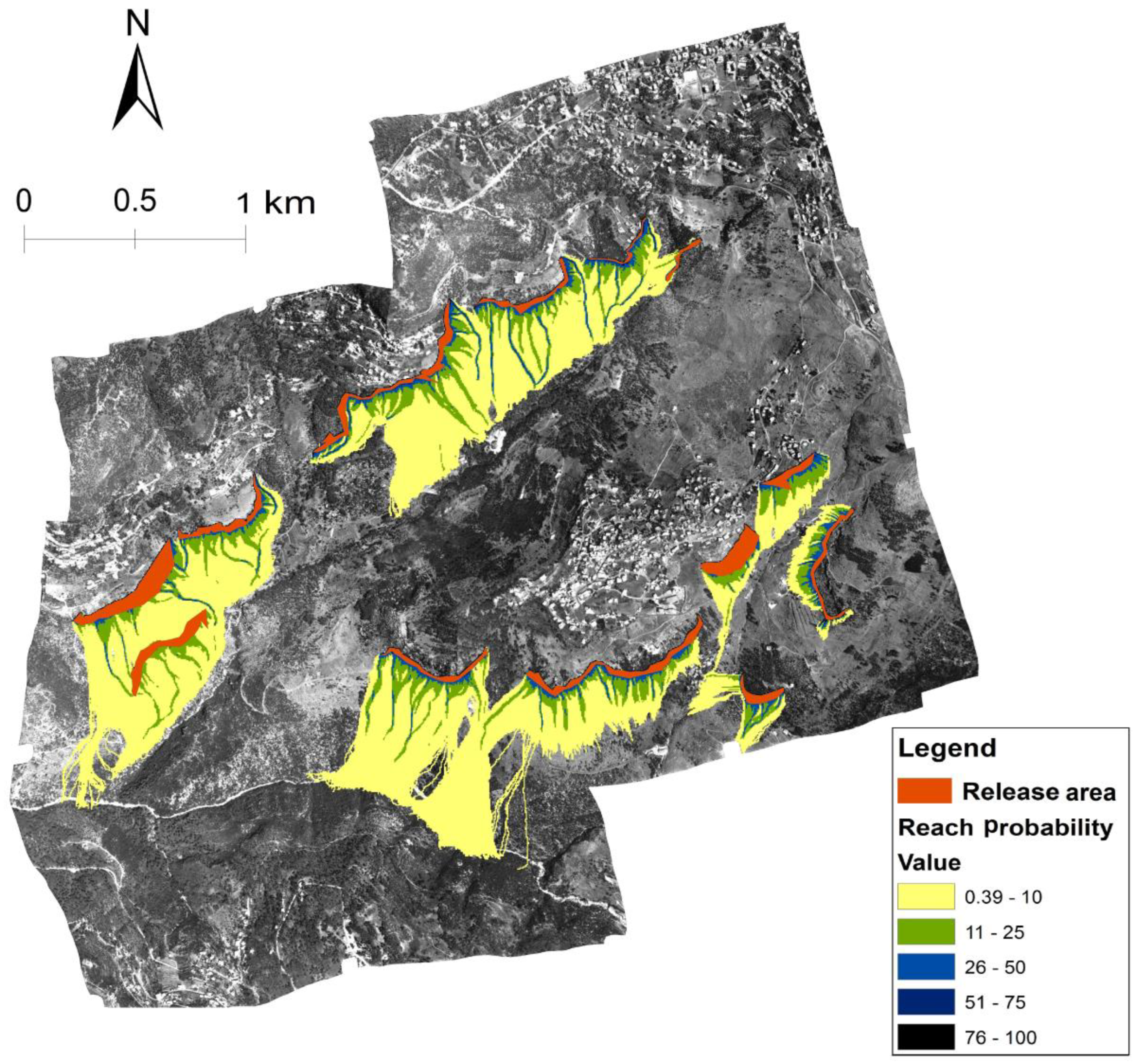
3. Results and Discussion

The study conducted in this paper presents a comparative analysis of the effects of three triggering factors for RFs (gravity, earthquakes and wet conditions). To the best of the author’s knowledge, this comparison was not conducted in previous studies of the scientific literature. Some similarities exist between this study and previous ones in terms of assessing the effects of the soil water content/moisture on RFs. Nevertheless, this study extended the scope of the investigation by differentiating between the effects of moisture content in rocks (water infiltration in the rock boulders) as well as in the soil.
The maps of the maximum deposited number of rocks are presented in Figure 9 in the case of earthquake-induced RFs; Figure 10 in the case of gravity-induced RFs; and in Figure 11 in the case of RFs induced by high water contents. The results corresponding to the earthquake effects indicate that most of the rocks have moved from the release areas and reached the accumulation zones with a large number (in red) of RFs (Figure 9). The results corresponding to the gravity effects indicate that a large number of RFs remain in the release areas in addition to noticeably large RFs gathered in the accumulation zones (Figure 10). The map showing the reach probability is presented in Figure 12. The distribution of the maximum deposited number of rocks, as well as the kinetic energy, are presented in Figure 13. To simplify the comparison of the results, the study area was divided into seven sub-areas, as shown in Figure 6. Different runout distances were observed in Figure 12 and this is explained by the diversity of topographic aspects, the slope profile, the slope materials and obstacles along the slope.

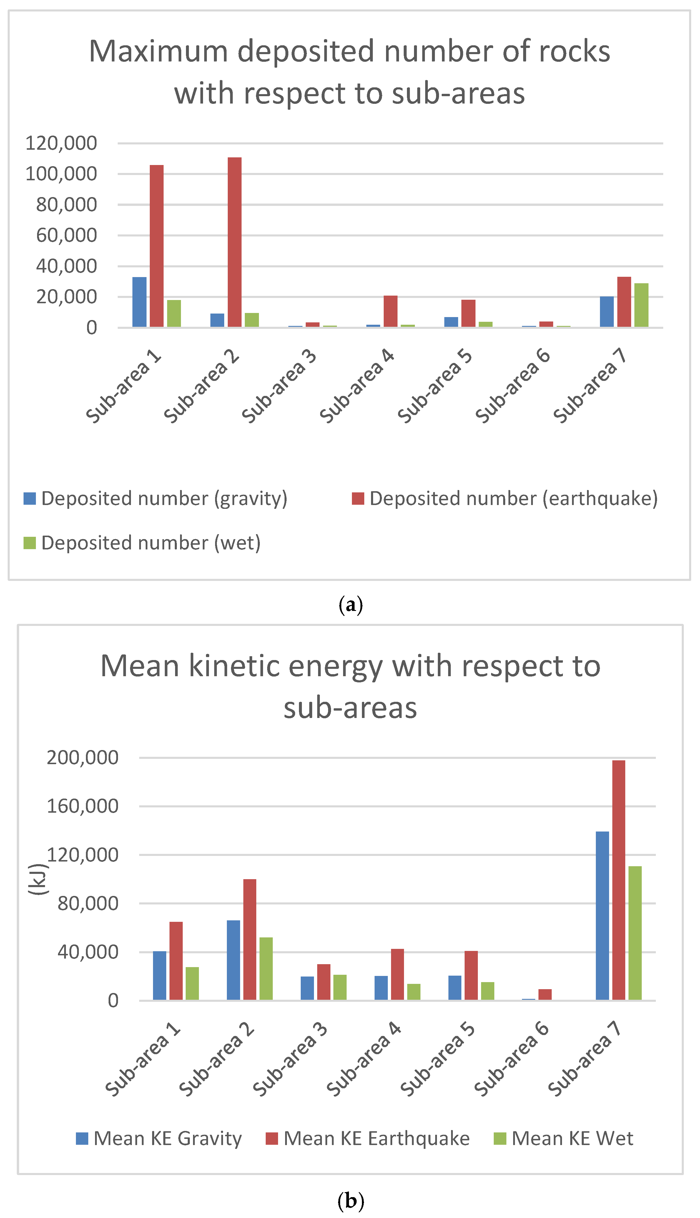
3.1. Mean Kinetic Energy

The case of RFs induced by gravity shows that the mean kinetic energy for each sub-area ranges between 1393 Kilojoules (kJ) (as in sub-area 6) and 139,109 kJ (as in sub-area 7). In the case of earthquake-induced RFs, the mean kinetic energy range is between 9266 kJ (as in sub-area 6) and 197,927 kJ (in sub-area 7). For the wet condition scenario, the mean kinetic energy was found to range between 602 kJ (in sub-area 6) and 110,716 kJ (in sub-area 7). When compared to gravity-induced RFs, the mean kinetic energy in the case of wet conditions was found to decrease by 43% and 79% in sub-areas 6 and 7, respectively. However, the ratios of the mean kinetic energy in the case of the earthquake to that of gravity-induced RFs are 6 and 1.4 in sub-areas 6 and 7, respectively. These results show that earthquakes would lead to RFs with higher energy and consequently longer runout distances relative to gravity-induced RFs. In contrast, moisture has a damping effect on RFs by decreasing the kinetic energy. An exceptional case was observed in sub-area 3 (sandstone lithology), where the mean kinetic energy in wet conditions (21,197 kJ) has slightly increased when compared to the gravity case (19,770 kJ). The exception could be referred to the hypothesis considering that low rock density, such as sandstone rocks, reverses slightly the effect of moisture factor on RFs kinetic energy, in the case of limestone rocks. This hypothesis needs to be validated by performing additional experiments.

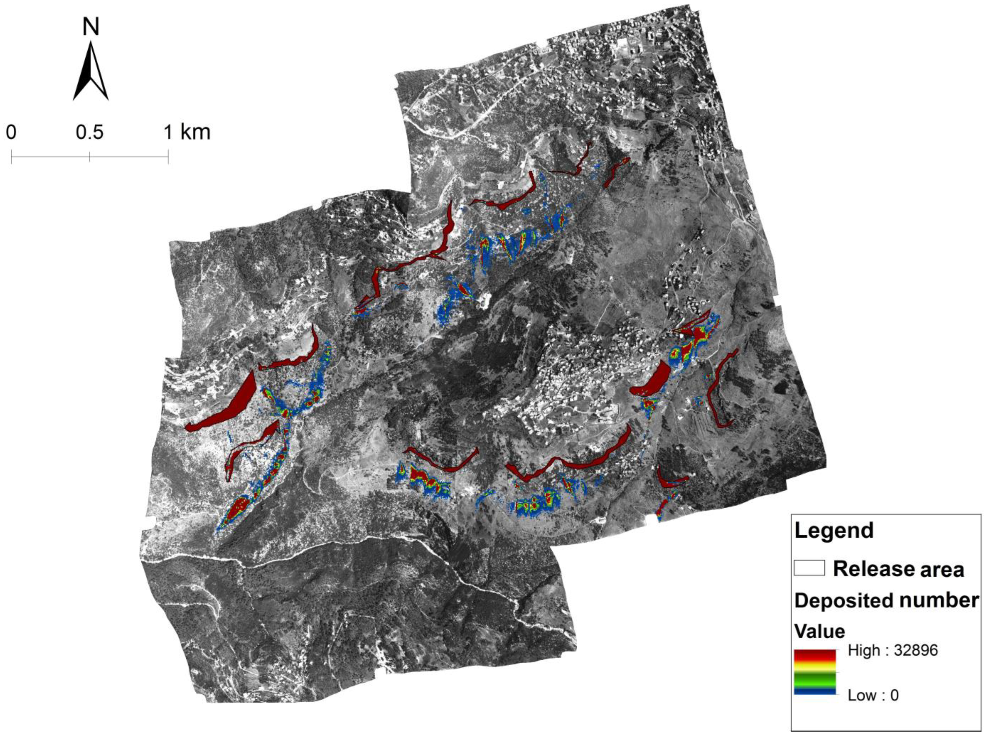
3.2. Maximum Deposited Rocks

In order to compare all the possibilities for RFs’ deposition number and deposition locations under the three proposed scenarios, thousands of simulations at the pixel level were conducted in order to increase the accuracy of the comparison process. The highest number of deposited rocks in the case of gravity was observed in sub-area 1 (32,896). In case of an earthquake, the maximum number (110,780) of deposited boulders was obtained in sub-area 2. The lower number of deposited rocks was observed in wet conditions, where the highest number of deposited rocks was in sub-area 7 (28,786). When looking at the distribution of deposited rocks, it is noted that in sub-areas 1 and 2, the case of the earthquake has dramatically increased the number of deposited rocks when compared to gravity-induced and case of wet conditions. This would be explained by the idea that the earthquake activated existing release areas that needed this amount of energy to launch rock falls. This is only a hypothesis that needs to be further tested in future research. The output raster maps of the Rockyfor3D, as well as the simulation results, showed that the effects of the earthquake/seismic induced RF could be depicted as increasing the kinetic energy of the RFs and, as a result, increasing the runout distances. In addition, the simulations showed that the earthquakes could be able to trigger the RF in new release areas when compared to RFs induced by gravity. On the other side, the effects of the wet conditions and moisture could be represented by a damping effect in soils. For instance, the mean kinetic energy in sub-area 1 in the case of wet conditions (27,425 kJ) is less than the one in the gravity-induced case (40,565 kJ) and the earthquake-induced case (64,775 kJ). This is caused by dissipating and reducing the forces required to trigger the RF and to push/move rocks (explained as the additional absorption of falling shock/impact within the moisturized soil), coupled with an increase in the boulders’ densities. In fact, increasing the rock density adds extra mass to the blocks, making them heavier and harder to move.

4. Conclusions

RF hazard is a natural phenomenon that could frequently occur in mountainous areas and represents a major threat to life, properties and infrastructure. For instance, in the study area, which is prone to high RF hazard, the land use maps displayed an accelerated urban development and indicated a lack of adequate urban planning. This raises the question about the risk assessments and measures relevant to RFs within local plans, in addition to triggering factors that affect the mechanism of RFs. This is why recent studies are aiming for a better understanding of this complicated mechanism to mitigate the negative effects of this natural hazard. This article presents the development of a new method to compare the effects of earthquakes and moisture on RF hazard.
The simulation results show that RFs are affected and triggered by several factors. According to the results obtained and by comparison, it was found that earthquakes increase the kinetic energy and lead to the highest number of rock deposition/falling, which represent the highest risk for humans and infrastructure. In contrast, wet conditions showed a damping effect when the soil is moisturized, but also showed that fully moisture-saturated rocks may slightly increase the kinetic energy of RFs, uncovering a new perspective on looking at RFs in wet conditions. Historical aerial photos proved their credibility to be the foundation of this work, especially when field observations confirmed the interpretation of aerial photos since the rock boulders did not show any sign of new movement during the 20 year period. Historical aerial photos showed their effectiveness in RF hazard studies; after orthorectification, they allowed us to precisely determine the distribution of RFs scattered all over the study area. It was used as a base map for the identification and mapping of rock distribution. The developed methodology and the corresponding produced maps could provide additional information and guidance for decision-makers during the phase of enacting new policies for urban planning and risk mitigation, especially in the cases of potential earthquakes and excessive soil moisturizing due to precipitation. Furthermore, although these maps express the spatial occurrence of the RF, their main limitation is that they do not include any information about the frequency and temporal occurrence of this natural hazard. The next step for developing this method is to determine the temporal occurrence, and an enhancement of the simulation is recommended by integrating more geotechnical and instability factors related to the initiation of RFs.

Author Contributions

Conceptualization, M.A.-S. and J.A.-G.; methodology, M.A.-S., J.A.-G. and W.A.-S.; software, M.A.-S. and G.F.; validation, M.A.-S., W.A.-S., J.A.-G., G.F. and P.-C.G.; formal analysis, M.A.-S. and W.A.-S.; investigation, M.A.-S.; resources, J.A.-G. and P.-C.G.; data curation, M.A.-S.; writing—original draft preparation, M.A.-S.; writing—review and editing, M.A.-S., W.A.-S., J.A.-G., G.F. and P.-C.G.; visualization, M.A.-S. and W.A.-S.; supervision, J.A.-G.; project administration, J.A.-G. and P.-C.G. All authors have read and agreed to the published version of the manuscript.

Funding

This research received no external funding.

Data Availability Statement

The data presented in this study are available on request from the corresponding authors.

Conflicts of Interest

The authors declare no conflict of interest.

References

  1. Farvacque, M.; Lopez-Saez, J.; Corona, C.; Toe, D.; Bourrier, F.; Eckert, N. Quantitative Risk Assessment in a Rockfall-Prone Area: The Case Study of the Crolles Municipality (Massif de La Chartreuse, French Alps). Géomorphol. Relief Process. Environ. 2019, 25, 7–19. [Google Scholar] [CrossRef]
  2. Lopez-Saez, J.; Corona, C.; Eckert, N.; Stoffel, M.; Bourrier, F.; Berger, F. Impacts of Land-Use and Land-Cover Changes on Rockfall Propagation: Insights from the Grenoble Conurbation. Sci. Total Environ. 2016, 547, 345–355. [Google Scholar] [CrossRef] [PubMed]
  3. Ferrari, F.; Giacomini, A.; Thoeni, K. Qualitative Rockfall Hazard Assessment: A Comprehensive Review of Current Practices. Rock Mech. Rock Eng. 2016, 49, 2865–2922. [Google Scholar] [CrossRef]
  4. Guzzetti, F.; Carrara, A.; Cardinali, M.; Reichenbach, P. Volcanic Events [3010 Yr Stern, 1991] and One of the NAVZ (Northern Austral Vol- Canic Zone). Geomorphology 1995, 13, 1995. [Google Scholar]
  5. Reichenbach, P.; Rossi, M.; Malamud, B.D.; Mihir, M.; Guzzetti, F. A Review of Statistically-Based Landslide Susceptibility Models. Earth-Sci. Rev. 2018, 180, 60–91. [Google Scholar] [CrossRef]
  6. Kakavas, M.; Nikolakopoulos, K. Digital Elevation Models of Rockfalls and Landslides: A Review and Meta-Analysis. Geosciences 2021, 11, 256. [Google Scholar] [CrossRef]
  7. Dorren, L.K.A. A Review of Rockfall Mechanics and Modelling Approaches. Prog. Phys. Geogr. 2003, 27, 69–87. [Google Scholar] [CrossRef] [Green Version]
  8. Ansari, M.K.; Ahmad, M.; Singh, R.; Singh, T.N. Rockfall Slope Angle and Its Effect on the Impact and Runout Distance of Falling Block: A Numerical Approach. In Proceedings of the 6th Indian Rock Conference, Mumbai, India, 17–18 June 2016. [Google Scholar]
  9. Wegner, K.; Haas, F.; Heckmann, T.; Mangeney, A.; Durand, V.; Villeneuve, N.; Kowalski, P.; Peltier, A.; Becht, M. Assessing the Effect of Lithological Setting, Block Characteristics and Slope Topography on the Runout Length of Rockfalls in the Alps and on the Island of La Réunion. Nat. Hazards Earth Syst. Sci. 2021, 21, 1159–1177. [Google Scholar] [CrossRef]
  10. Sala, Z.; Hutchinson, D.J.; Harrap, R. Simulation of Fragmental Rockfalls Detected Using Terrestrial Laser Scans from Rock Slopes in South-Central British Columbia, Canada. Nat. Hazards Earth Syst. Sci. 2019, 19, 2385–2404. [Google Scholar] [CrossRef] [Green Version]
  11. Wei, L.-W.; Chen, H.; Lee, C.-F.; Huang, W.-K.; Lin, M.-L.; Chi, C.-C.; Lin, H.-H. The Mechanism of Rockfall Disaster: A Case Study from Badouzih, Keelung, in Northern Taiwan. Eng. Geol. 2014, 183, 116–126. [Google Scholar] [CrossRef]
  12. Saroglou, C.; Asteriou, P.; Zekkos, D.; Tsiambaos, G.; Clark, M.; Manousakis, J. UAV-Based Mapping, Back Analysis and Trajectory Modeling of a Coseismic Rockfall in Lefkada Island, Greece. Nat. Hazards Earth Syst. Sci. 2018, 18, 321–333. [Google Scholar] [CrossRef]
  13. Kobayashi, Y.; Harp, E.L.; Kagawa, T. Simulation of Rockfalls Triggered by Earthquakes. Rock Mech. Rock Eng. 1990, 23, 1–20. [Google Scholar] [CrossRef]
  14. Valagussa, A.; Frattini, P.; Crosta, G.B. Earthquake-Induced Rockfall Hazard Zoning. Eng. Geol. 2014, 182, 213–225. [Google Scholar] [CrossRef]
  15. Koukouvelas, I.; Litoseliti, A.; Nikolakopoulos, K.; Zygouri, V. Earthquake Triggered Rock Falls and Their Role in the Development of a Rock Slope: The Case of Skolis Mountain, Greece. Eng. Geol. 2015, 191, 71–85. [Google Scholar] [CrossRef]
  16. Vick, L.M.; Zimmer, V.; White, C.; Massey, C.; Davies, T. Significance of Substrate Soil Moisture Content for Rockfall Hazard Assessment. Nat. Hazards Earth Syst. Sci. 2019, 19, 1105–1117. [Google Scholar] [CrossRef] [Green Version]
  17. Duarte, R.M.; Marquínez, J. The Influence of Environmental and Lithologic Factors on Rockfall at a Regional Scale: An Evaluation Using GIS. Geomorphology 2002, 43, 117–136. [Google Scholar] [CrossRef]
  18. Jones, C.L.; Higgins, J.D.; Andrew, R.D. Higgins, Colorado Rockfall Simulation Program Version 4.0 Manual; Colorado Department of Transportation: Denver, CO, USA, 2000; p. 80222.
  19. Rocscience Inc. RocFall Version 4.0–Statistical Analysis of Rockfalls. 2021. Available online: https://www.rocscience.com (accessed on 25 September 2022).
  20. Guzzetti, F.; Crosta, G.; Detti, R.; Agliardi, F. STONE: A Computer Program for the Three-Dimensional Simulation of Rock-Falls. Comput. Geosci. 2002, 28, 1079–1093. [Google Scholar] [CrossRef]
  21. RocPro3D. RocPro3D Software. 2014. Available online: http://www.rocpro3d.com/rocpro3den.php (accessed on 25 September 2022).
  22. Bartelt, P.; Bieler, C.; Bühler, Y.; Christen, M.; Christen, M.; Dreier, L.; Gerber, W.; Glover, J.; Schneider, M.; Glocker, C.; et al. RAMMS::ROCKFALL User Manual v1.6, 102; WSL Institute for Snow and Avalanche Research SLF: Davos, Switzerland, 2016. [Google Scholar]
  23. Bunce, C.M.; Cruden, D.M.; Morgenstern, N.R. Assessment of the Hazard from Rock Fall on a Highway. Can. Geotech. J. 1997, 34, 344–356. [Google Scholar] [CrossRef]
  24. Cancelli, A.; Crosta, G. 15. Hazard and Risk Assessment in Rockfall Prone Areas. In Risk and Reliability in Ground Engineering; Thomas Telford Publishing: London, UK, 1993; pp. 177–190. [Google Scholar]
  25. Zheng, L.; Wu, Y.; Zhu, Z.; Ren, K.; Wei, Q.; Wu, W.; Zhang, H. Investigating the Role of Earthquakes on the Stability of Dangerous Rock Masses and Rockfall Dynamics. Front. Earth Sci. 2022, 9, 1338. [Google Scholar] [CrossRef]
  26. Faour, G. Forest Fire Fighting in Lebanon Using Remote Sensing and GIS; Techinal Report; Association for Forest Development and Conservation Commission: Amaret Chalhoub, Lebanon, 2016. [Google Scholar]
  27. Dubertert, L. Geological Maps of Syria and Lebanon at 1.50.000. 21 Sheets with Explicative Note; Minister of public affairs, Damas and Beirut; Google: Menlo Park, CA, USA, 1953. [Google Scholar]
  28. Ozturk, D. Urban Growth Simulation of Atakum (Samsun, Turkey) Using Cellular Automata-Markov Chain and Multi-Layer Perceptron-Markov Chain Models. Remote Sens. 2015, 7, 5918–5950. [Google Scholar] [CrossRef] [Green Version]
  29. Weng, Q. Remote Sensing and GIS Integration; McGraw-Hill Professional Publishing: New York, NY, USA, 2010. [Google Scholar]
  30. Albarelli, D.S.N.A.; Mavrouli, O.C.; Nyktas, P. Identification of Potential Rockfall Sources Using UAV-Derived Point Cloud. Bull. Eng. Geol. Environ. 2021, 80, 6539–6561. [Google Scholar] [CrossRef]
  31. Walstra, J.; Chandler, J.H.; Dixon, N.; Dijkstra, T.A. Aerial Photography and Digital Photogrammetry for Landslide Monitoring. Geol. Soc. Lond. Spec. Publ. 2007, 283, 53–63. [Google Scholar] [CrossRef]
  32. Fanos, A.M.; Pradhan, B. Laser Scanning Systems and Techniques in Rockfall Source Identification and Risk Assessment: A Critical Review. Earth Syst. Environ. 2018, 2, 163–182. [Google Scholar] [CrossRef]
  33. Scaioni, M.; Longoni, L.; Melillo, V.; Papini, M. Remote Sensing for Landslide Investigations: An Overview of Recent Achievements and Perspectives. Remote Sens. 2014, 6, 9600–9652. [Google Scholar] [CrossRef] [Green Version]
  34. Buill, F.; Núñez-Andrés, M.A.; Lantada, N.; Prades, A. Comparison of Photogrammetric Techniques for Rockfalls Monitoring. IOP Conf. Ser. Earth Environ. Sci. 2016, 44, 042023. [Google Scholar] [CrossRef] [Green Version]
  35. Chandler, J.H.; Moore, R. Analytical Photogrammetry: A Method for Monitoring Slope Instability. Q. J. Eng. Geol. Hydrogeol. 1989, 22, 97–110. [Google Scholar] [CrossRef]
  36. Abou-Jaoude, G.; Saade, A.; Wartman, J.; Grant, A. Earthquake-Induced Landslide Hazard Mapping: A Case Study in Lebanon. In Geo-Chicago; American Society of Civil Engineers: Chicago, IL, USA, 2016; pp. 177–186. [Google Scholar]
  37. Rocchini, D.; Metz, M.; Frigeri, A.; Delucchi, L.; Marcantonio, M.; Neteler, M. Robust Rectification of Aerial Photographs in an Open Source Environment. Comput. Geosci. 2012, 39, 145–151. [Google Scholar] [CrossRef]
  38. Schneider, C.A.; Rasband, W.S.; Eliceiri, K.W. NIH Image to ImageJ: 25 Years of Image Analysis. Nat. Methods 2012, 9, 671–675. [Google Scholar] [CrossRef]
  39. Federal Geographical Data Committee. Geospatial Positioning Accuracy Standards Part 3: National Standard for Spatial Data Accuracy; National Aeronautics and Space Administration: Virginia, NV, USA, 1998; p. 28.
  40. Brunetti, M.T.; Guzzetti, F.; Rossi, M. Probability Distributions of Landslide Volumes. Nonlinear Process. Geophys. 2009, 16, 179–188. [Google Scholar] [CrossRef] [Green Version]
  41. Guzzetti, F.; Reichenbach, P.; Wieczorek, G.F. Rockfall Hazard and Risk Assessment in the Yosemite Valley, California, USA. Nat. Hazards Earth Syst. Sci. 2003, 3, 491–503. [Google Scholar] [CrossRef] [Green Version]
  42. Ritchie, A.M. Evaluation of Rockfall and Its Control. In Highway Research Record; Highway Research Board, National Research Council: Washington, DC, USA, 1963; pp. 13–28. [Google Scholar]
  43. Darwish, T.; Lebanese National Council for Scientific Research Remote Sensing Center. Soil Map of Lebanon 1:50,000; CNRS, Remote Sensing Center: Beirut, Lebanon, 2006. [Google Scholar]
  44. Khatiwada, D.; Dahal, R.K. Rockfall Hazard in the Imja Glacial Lake, Eastern Nepal. Geoenvironmental Disasters 2020, 7, 29. [Google Scholar] [CrossRef]
  45. Dorren, L.K.A. Rockyfor3D (v5.2) Revealed—Transparent Description of the Complete 3D Rockfall Model; ecorisQ Paper; Int. ecorisQ Association: Geneva, Switzerland, 2016; 33p, Available online: https://wwwecorisq.org/tool-manuals/rockyfor3d-user-manual/3-english/file (accessed on 25 September 2022).
  46. Elias, A. Short Notice on Earthquake Hazard in Lebanon; Geology Department, American University of Beirut: Beirut, Lebanon, 2012. [Google Scholar]
  47. Harajli, M.; Sadek, S.; Asbahan, R. Evaluation of the Seismic Hazard of Lebanon. J. Seismol. 2002, 6, 257–277. [Google Scholar] [CrossRef]
  48. Mavrouli, O.; Corominas, J.; Wartman, J. Methodology to Evaluate Rock Slope Stability under Seismic Conditions at Solá de Santa Coloma, Andorra. Nat. Hazards Earth Syst. Sci. 2009, 9, 1763–1773. [Google Scholar] [CrossRef] [Green Version]
  49. Rabat, R.; Tomás, R.; Cano, M.; Pérez-Rey, I.; Siles, J.S.; Alejano, L.R. Influence of Water Content on the Basic Friction Angle of Porous Limestones—Experimental Study Using an Automated Tilting Table. Bull. Eng. Geol. Environ. 2022, 81, 223. [Google Scholar] [CrossRef]
  50. El-Sohby, M.A.; Aboushook, M.I. Slope Degradation and Analysis of Mokattam Plateau, Egypt. In Proceedings of the 2nd International Conference on Geotechnical Site Characterization, Porto, Portugal, 19–22 September 2004; pp. 1081–1887. [Google Scholar]
  51. Asteriou, P.; Saroglou, H.; Tsiambaos, G. Rockfall: Scaling Factors for the Coefficient of Restitution. In Proceedings of the ISRM International Symposium-EUROCK 2013, Wroclaw, Poland, 23–26 September 2013; p. 195. [Google Scholar]
  52. Robert, S.; Klein, C.; Carmichael. General Considerations Rock Types, Rock. Encycl. Br. 1. 2021. Available online: https://www.britannica.com/science/rock-geology (accessed on 25 September 2022).
Figure 1. Study area.
Geographies 03 00006 g001
Figure 2. Land use maps of the study area for the years 1999 and 2020.
Geographies 03 00006 g002
Figure 3. Construction built on rockfalls.
Geographies 03 00006 g003
Figure 4. Massive rock boulders standing just above the buildings and the release area is just above.
Geographies 03 00006 g004
Figure 5. Developed methodology.
Geographies 03 00006 g005
Figure 6. Map of the past falling blocks.
Geographies 03 00006 g006
Figure 7. A sketch showing the obstacle heights (MOH) that account for 70%, 20%, and 10% of the slope’s surface, respectively. The MOH should be measured while looking downward, modified after (Rockyfor3D manual [45]).
Geographies 03 00006 g007
Figure 8. Simulations’ process.
Geographies 03 00006 g008
Figure 9. The obtained deposited number of rocks after 1000 simulations for the worst case scenario: earthquake with magnitude 7.
Geographies 03 00006 g009
Figure 10. The obtained deposited number of rocks after 1000 simulations for the case scenario: gravity-induced.
Geographies 03 00006 g010
Figure 11. The obtained deposited number of rocks after 1000 simulations for the case scenario: wet condition.
Geographies 03 00006 g011
Figure 12. Reach probabilities obtained after 1000 simulations for the worst case scenario: earthquake with magnitude 7.
Geographies 03 00006 g012
Figure 13. (a) Maximum deposited number of rocks with respect to sub-areas; (b) mean kinetic energy with respect to sub-areas.
Geographies 03 00006 g013
Disclaimer/Publisher’s Note: The statements, opinions and data contained in all publications are solely those of the individual author(s) and contributor(s) and not of MDPI and/or the editor(s). MDPI and/or the editor(s) disclaim responsibility for any injury to people or property resulting from any ideas, methods, instructions or products referred to in the content.

