
Hydrological Responses to Land Use/Land Cover Changes in Koga Watershed, Upper Blue Nile, Ethiopia

1
Department of Hydraulic and Water Resources Engineering, Bule Hora University (BHU), Bule Hora P.O. Box 144, Ethiopia
2
Department of Water Works Construction Technology, Faculty of Civil Technology, Ethiopia Technical University, 2RGF + MHJ, Addis Ababa P.O. Box 190310, Ethiopia
3
Department of Natural Resources Management, Arba Minch University, Arba Minch P.O. Box 21, Ethiopia
*
Author to whom correspondence should be addressed.
Geographies 2023, 3(1), 60-81; https://doi.org/10.3390/geographies3010004
Submission received: 20 November 2022
/
Revised: 30 December 2022
/
Accepted: 4 January 2023
/
Published: 10 January 2023
(This article belongs to the Special Issue A GIS Spatial Analysis Model for Land Use Change (Volume II))
Abstract
:Information on land use and land cover modification and their related problems for the streamflow and sediment yield are crucial for spatial planners and stakeholders to devise suitable catchment resources management plans and strategies. This research sought to assess the changes in land use and land cover (LULC) effects on the streamflow and sediment yield of the Koga watershed. Landsat-5 TM, Landsat-7 ETM+, and Landsat-8 OLI data were used to create the land use and land cover maps. The LULC type identification analysis was performed by using ERDAS Imagine 2015. After the supervised classification, the land use and land cover maps for three distinct years (1991, 2008, and 2018) were generated, and the accuracy of the maps was reviewed. The LULC change analysis results were pointed out, as there was an appreciable LULC change in the study watershed. Agricultural land increased by 14.21% over the research period, whereas grassland decreased by 22.91%. The other LULC classes (built-up area, forest area, water body, and wetland) increased by 0.39%, 6.36%, 4.30%, and 0.46%, respectively. Contrarily, bushland decreased by 2.80%. Human activities were decisive in the significant land use alterations within the catchment. The flow rate of the river basin increased over the rainy season in the years 1991–2008 and declined in the drier months. The watershed’s sediment yield increased from 1991 to 2008 as a result of the extension of its agricultural area. Thus, the findings of this investigation demonstrated that the flow and sediment yield characteristics are changed because of the modifications within the LULC in the catchment. Some downstream and upstream parts of the area are exposed to comparatively high erosion, and the maximum amount of sediment is generated during the rainy season.
1. Introduction
Water is a valuable resource, which is required for all forms of socioeconomic development and which must be managed sustainably to suit both human and environmental needs [1]. However, water resources are affected by many parameters. The land use and land cover of the watershed area are among the principal factors affecting the amount of flow in the catchment [2,3].
Changes in land use and cover are an unavoidable and significant worldwide ecological trend [4]. The modification in land use/cover influences evaporation, groundwater infiltration, overland runoff, sedimentation rate, and the streamflow of the watershed by changing the magnitude and pattern of surface runoff, groundwater flow, and soil moisture content [5,6]. The catchment’s sediment output and the flow available for both ecosystem function and human usage are specifically influenced by changes in land use/cover [7,8,9,10,11]. Consequently, a reduced availability of several goods and services for people, animals, and agricultural output could result from LULC modification, which could also have an impact on the environment [12,13].
At the global, regional, and local levels, land use/cover change has emerged as a significant environmental concern [14,15]. It is also a challenge in Ethiopia [16,17,18,19]. The change in LULC was the cause of streamflow changes in the country [20]. The low fertile soils and induced siltation in lakes and reservoirs are generated from the mountainous Ethiopian highlands. Thus, the entire upper Blue Nile Basin has been extensively impacted by soil erosion and siltation activities [21,22,23].
The impacts related to sedimentation and water resources of the catchment originating from the inevitable land use and land cover change are a significant problem and the most crucial research concern worldwide [23,24,25,26,27,28]. These influences are mainly reflected by changes in the aspects of erosion rate, water cycle, and water quantity [29,30,31,32,33,34]. Poor land use patterns and insufficient management methods have affected the pace of soil erosion, the movement of sediment, and the loss of agricultural nutrients in the Ethiopian highlands [35,36]. To meet the demands of an expanding society, a widening of cultivation activity, urban expansion, the removal of timber and other natural resources are probably going to increase over the next few decades [37].
The most significant issues in the Koga watershed are also soil erosion and the ensuing land degradation [38]. In this watershed, the majority of the supplying sub-catchments are very erodible; large amounts of coarse sediments have accumulated in the river channel, which in turn affects the life expectancy of the Koga dam [39]. For instance, the Koga dam, built in the Koga watershed, is one of the seriously damaged dams in the Blue Nile Basin; siltation also reduces the reservoir’s ability to store water [39,40]. Around 7000 hectares of land was intended to be irrigated as part of the Koga irrigation project. Presently, only 6000 ha of the land is irrigated, and the remaining 1000 ha of the land is suffering from a shortage of water [41,42]. This irrigated land affects both the aim of the project and the economy of the government/society.
A thorough understanding of the LULC change is helpful for reconstructing previous LULC changes, predicting future changes for adequate and sustainable streamflow and decreased sediment depositions, and developing sustainable land resource management techniques intended to protect essential landscape functioning. This knowledge turns into crucial information for producing evidence that helps local communities, actors functioning within a given environment, spatial planners, and decision makers to design the best policies and strategies. An understanding of the extent of sediment deposition in the rivers/reservoirs and knowing the changes in streamflow are necessary for an effective reservoir and basin management program [43].
The overall objective of this research is to evaluate the effects of land use and land cover change on the streamflow and sediment yield of the Koga watershed. Local governments and stakeholders would benefit greatly from learning more about how LULC change affects the flow and sediment production of the Koga watershed in order to develop and implement efficient watershed management strategies, as well as minimizing upcoming land use changes. To perform the analysis, hydrological models play a vital role in simulating the real-world hydrologic processes. These hydrological models are very important to understand and explain the effects of LULC changes on the hydrologic responses of a catchment [44]. The physically based semi-distributed hydrologic tool (SWAT), one of such models, is employed to determine how land use modification affects the flow and sediment regimes of the watershed under various soil, land use, and management situations over a longer period [45]. By combining a variety of pertinent geographic data, SWAT can accurately characterize the watershed, and the model is compatible with ArcGIS [46].
2. Materials and Methods
2.1. Study Area Description
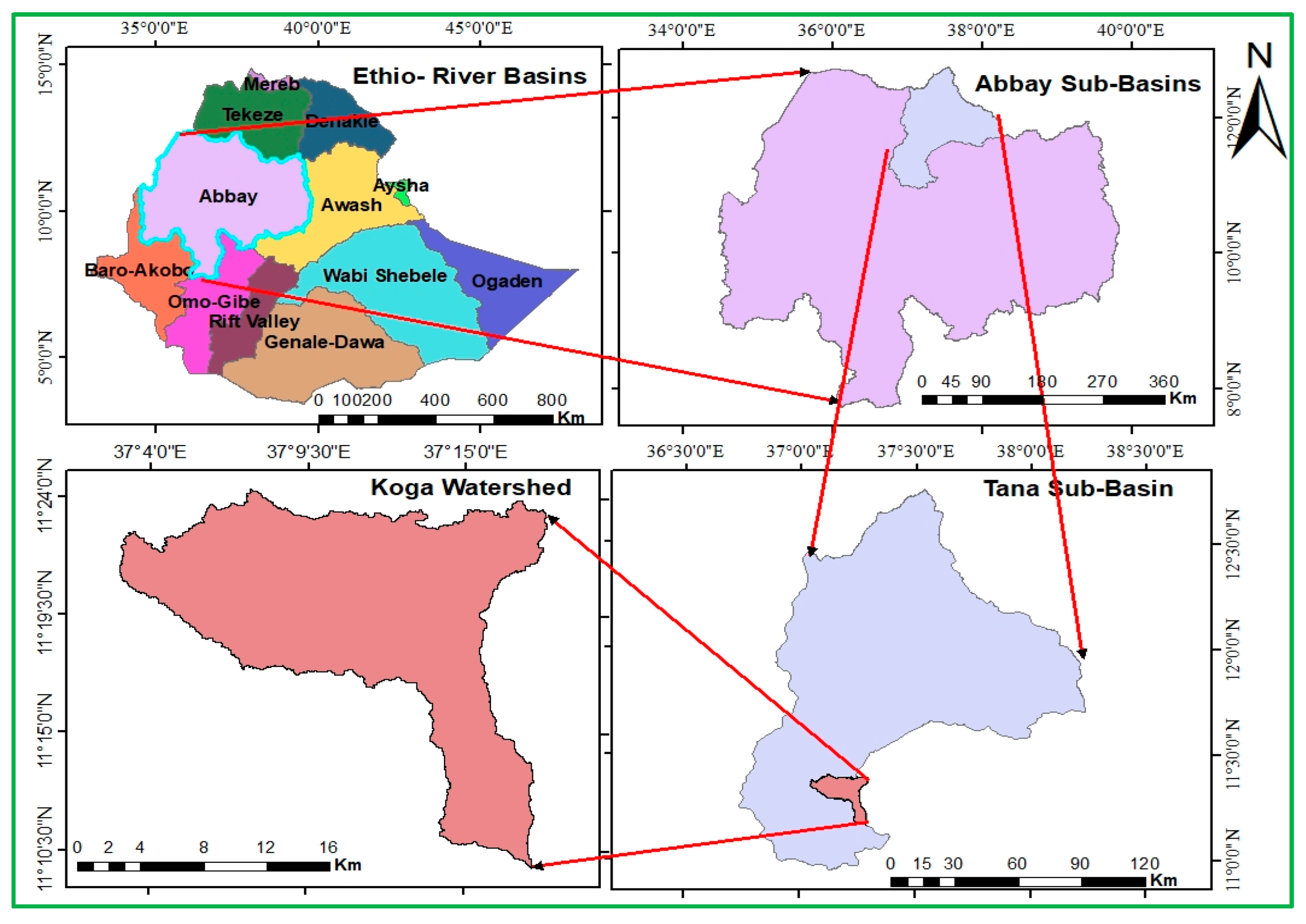
The Koga watershed has an approximate drainage area of about 301.20 Km2 and is located in the northern part of Ethiopia, from 11°10′ to 11°25′ N and 37°00′ to 37°20′ (Figure 1). In the region of the Blue Nile basin above, the Koga River joins the Gilgel Abbay River, a tributary of Lake Tana. The catchment is narrow and steep upstream while being wide and nearly flat downstream. Eutric vertisols, haplic luvisols, haplic alisols, haplic nitisols, and lithic leptosols are the primary types of soil found in the Koga watershed. Among these, haplic luvisol and haplic alisols cover the wider area of the watershed. The Koga catchment is situated in both the Woina Dega and Dega zones. The wider area from the catchment is enclosed in the Woina Dega zone [47]. The rainfall totals for the watershed range from 1247.07 to 1846.30 mm annually. The range for the average yearly highest and lowest temperatures is 22.25 to 27.44, and 9.45 to 12.70 °C, respectively. The Koga watershed’s LULC are primarily dominated by agricultural activity. Other land use/cover types included in the watershed are grassland, forest cover, wetland, bushland, settlement/built-up area, and water body.
2.2. Data Collection
2.2.1. Spatial Data
Digital Elevation Model
The USA Geology Survey acquired the Digital Elevation Model (DEM) from the Shuttle Radar Topography Mission utilizing the appropriate data required for the SWAT model.
Soil Data
The Ministry of Water Resources, Irrigation, and Electricity (MoWIE) provided the soil data, and it is highly relevant for the SWAT tool to provide both the distribution of soil types in the catchments and the various parameters describing the soil’s hydrological and textural properties. Among the soil types in the Koga watershed, haplic luvisol and haplic alisols cover the dominant part of the watershed. Haplic luvisols predominantly cover the downstream portion of the watershed, while haplic alsisols predominantly cover the upstream portion.
Land Use/Cover Data
The satellite images for the years 1991 (Landsat -5 TM), 2008 (Landsat -7 ETM+), and 2018 (Landsat -8 OLI) were acquired from USGS Earth Explorer. The preference for the reference years depended on the political and social conditions, e.g., 1991, the upcoming FDRE regime, and the occurrence of large-scale war with the Derg regime. There was extensive planting and reforestation during the Ethiopian Millennium in 2008. The year 2018 was the start of the Ethiopian Growth and Transformation Plan (GTP-II) to enhance the agricultural productivity of the country. Concerning the periodic intervals of LULC modification, the time could not be too short; thus, the years 1991, 2008, and 2018 were taken as the reference years for the LULC change quantification. Images with a 30 m ∗ 30 m resolution were utilized in this study.
2.2.2. The Weather and Hydrological Data
Weather Data
From 1987 to 2018, the National Meteorological Service Agency of Ethiopia provided the daily weather data. These data were collected at seven nearby stations of the Koga watershed (i.e., Bahir Dar, Dangila, Adet, Merawi, Bahir Dar airport, Sekela, and Wetet Abbay stations) (Table 1).
Hydrological Data
The calibration and validation of the SWAT prediction result depend on the daily/monthly discharge data. These daily data for the years 1991 through 2008 are provided by Ethiopia’s Ministry of Water Resources, Irrigation, and Electricity. The flow information (18-year period of daily flow data) on Koga from the Merawi gauging station is used for this study.
Instead of data for all months and days, the sediment data from Ethiopia’s Ministry of Water Resources, Irrigation, and Electricity (MoWIE) are a sample taken on a concentration basis in different seasons over different years. Therefore, it was crucial to establish a relationship between river discharge and sediment load to generate daily sediment loads using the information at hand (sediment rating curve).
2.3. Data Analysis
2.3.1. Image Processing and Classification
Image processing is a technique for implementing some operations to obtain an enhanced image or to extract some relevant data from it. All the downloaded satellite images are georeferenced, and the image pre-processing tasks, such as gap filling, layer stacking, haze reduction, and band color combination, are carried out using ERDAS IMAGINE 2015 v15.0 software.
Image classification is the process of assigning pixels from a continuous raster image to already existing land cover classes [48]. Image classification is relevant for grouping similar pixel values together. It is also important to transform the pixel values directly into the classes of land use [49]. There are several image classification techniques in remote sensing. In most cases, three classification methods are found: supervised, unsupervised, and hybrid. A supervised classification approach needs some prior information about all relevant land cover classes in the image, while an unsupervised classification approach can be carried out without this information. In the unsupervised classification method, the iterative self-organizing data analysis (ISODATA) clustering algorithm is utilized [50]. Meanwhile, the maximum likelihood classification (MLC) algorithm is significantly used in the supervised classification approach by assembling the training areas for the LULC classes [51]. The hybrid classification technique embodies an unsupervised classification technique followed by a supervised classification technique [52].
The supervised classification method using the maximum likelihood classifier is used for this study. This method of classification automatically groups all pixels with comparable spectral values into distinct land use/cover classes or themes [53]. For conveying the spectral signature of recognized features, a manual distinction of the point of interest areas as a ground truth or reference within the images is required. In addition to ERDAS imagine 2015, Arc GIS 10.4 software is used for mapping and raster and vector data analysis. After the supervised classification and recording, the initial classified LULC map is modified based on the ground verification of any questionable locations.
2.3.2. Image Classification Accuracy Assessment
Accuracy evaluation is necessary to know whether the pixels are assigned to the perfect land use/cover classes or not. It is also relevant for evaluation of the classification method, and it is important to quantify the error that might be involved during the classification processes [54]. Accuracy evaluation using a confusion matrix is the most widely utilized accuracy assessment approach, which can be used to produce a series of explanatory and analytical information [55]. Hence, the accuracy assessment in this study is evaluated in the form of an error matrix.
The ground truths are acquired from Google Earth in order to guarantee the representativeness of the classified maps on the ground. The data utilized to verify the correctness of the classified maps include the kappa coefficient, overall accuracy, producer’s accuracy, and user’s accuracy. The kappa statistics (K) prove the agreement between the classified maps and reference points/ground truths. According to Ref [56], the recommended value of the kappa statistics is tabulated below (Table 2).
Following the accuracy assessment, some land use types are recoded into their correct classes. After executing all the steps above, the major LULC types are identified, and the LULC map is represented with the four-letter SWAT codes for distinct classes of land use/cover to link with the grid values of the SWAT model land use/cover database.
2.3.3. Weather and Hydrological Data Analysis
Data Quality Tests
The model will produce inaccurate results if incorrect data are used as input. In order to ensure their accuracy before being used for further analysis, the meteorological and flow data are checked. Visual inspection, filling in of missing data, finding outliers, cumulative plot, and double mass curve analysis are used to assess the quality of the data. Before the data are used for further analysis, this analysis is used to identify any gaps in the data and fill them in.
In this research, both the missing values of flow and weather data were filled by XLSTAT Perpetual 2019.2.2 statistical software for Excel. During the analysis, both the flow and weather data are checked for their outliers by using the Grubbs test method [57]. Finally, the data that are evaluated as outliers are rejected and filled as a missing value. The rain records are examined and revised using the double mass curve technique to adjust for non-representative events, such as a shift in the placement or exposure of the rain gauge. The modifications in the data’s statistical traits related to rainfall are validated by the homogeneity test, and hence, the group stations selected were homogenous. Equation (2) below was used to calculate the homogeneity of the selected gauging stations’ monthly rainfall records.
where
is the dimensionless monthly rainfall value for station-I;
is the annualized monthly rainfall value for station-I;
is station-I annual rainfall data averaged over the years.
Following the qualitative analysis and preparation of the lookup table for the weather data, the weather generator generated the full and realistic long-period data for SWAT input.
Sediment Data Analysis
The sediment data obtained from the Ministry of Water Resources, Irrigation, and Electricity (MoWIE) are a sample taken on a concentration basis over various seasons within various years rather than data for all months and days. Due to this, it was necessary to establish a relationship between river discharge and silt concentration in order to produce the daily sediment loads using the data already available. As a result, the sediment–rating curve is created for the station as follows:
where Q is the flow discharge (m3/s), and Qs is the concentration of suspended sediment (ton/day).
Qs = 15.794 ∗ Q1.5515 with an R2 = 0.87
2.4. SWAT Model Description
The soil and water assessment tool (SWAT) is a physically based semi-distributed hydrologic tool, which estimates how varied soil, land use, and management conditions affect the flow and sediment regimes of the watershed over a longer period [45]. According to Ref [58], the model can analyze the spatial detail of the catchment, and different scenarios can be simulated in this model. In addition to this, SWAT uses the available land use, soil, weather, and topographic data as input for further analysis.
A watershed is divided up into several sub-watersheds in SWAT, and each sub-land watershed’s areas are then further divided up into one or more land units. These distinct land units, in terms of soil qualities, land use, and management, are known as hydraulic response units (HRUs). A better estimation of the loadings (streamflow, sediment, pollutants) from the sub-basins is made possible by the HRUs [59]. The catchment elements, such as weather, sedimentation, hydrology, soil temperature, crop growth, nutrient, pesticides, and agricultural practices, can be simulated by the SWAT model [45]. The streamflow of the watershed is determined by surface runoff and groundwater flow from shallow aquifers [60]. Other models have not proven as successful as the SWAT approach [61,62]. Furthermore, SWAT (i.e., a semi-distributed model) has a more physical-based nature than lumped models. This model is freely accessible and capable of analyzing the spatial detail of the watershed.
2.4.1. The Hydrological Components of SWAT
There are two portions of hydrologic predictions in a certain watershed. The first is the land phase, which regulates water flow in the land and the amount of water, sediment, nutrients, and pesticides that are transmitted into the stream [63]. SWAT simulates the hydrologic cycle based on the water balance principle [64].
where t is the number of days, Rday is the quantity of rainfall on day-I, SWt is the soil water content (mm), SWo is the beginning water content (mm), Qsurf is the day-I surface runoff amount (mm), Ea is equal to the evapotranspiration on day-I (mm). Wseep is the quantity of water that seeps into the earth on day-I (mm), and Qgw is the day-I return flow quantity (mm).
The second phase of the hydrological cycle is the routing phase, during which the water is channeled through the local channel networks delivering sediment, nutrients, and pesticides to the exit [63]. The discharge in the channels can be routed by two methods: the available storage method and the Muskingum method. The water volume in the available storage method can be routed using the concept of a simple continuity equation. The Muskingum routing method makes substantial use of the wedge and prism storage concepts. The equation of the available storage routing is stated as
where is the volume change (m3 water), is the inflow volume (m3 water), and is the outflow volume (m3 water).
2.4.2. Sediment Component of SWAT
SWAT predicts soil erosion and siltation by applying the modified universal soil loss equation (MUSLE) [65].
where Qsurf is the amount of surface runoff, and Sed is the daily sediment production (in metric tons) (in millimeters per hectare). is the HRU’s area (in hectares), Qpeak is the peak runoff rate (in meters per second), PUSLE is the support practice factor, LSUSLE is the topographic factor, CUSLE is the cover factor, and CFRG is the coarse fragment factor. KUSLE is the soil erodibility factor, which is 0.013 metric ton m2 h/(m3-metric ton cm).
2.5. SWAT Model Setup and Watershed Delineation
Before running the SWAT model, there should be a model set up after all the input data are collected. During model setup, there are some procedures to be followed. These include situating an outlet where the streamflow gauging station is positioned. The information acquired from this outlet/station is relevant for model calibration and validation. Unnecessary outlets were removed for better sub-basin classification.
A watershed is defined as all points contained inside a region of land from which rainfall will provide the water to the outlet. The five essential steps in the watershed delineation process are: setting up the DEM; identifying the stream network; defining the outlet and inlet points; determining the watershed outlet(s); and determining the sub-basin parameters. Following the implementation of the DEM setup and the specification of the outflow point, the model automatically generates the flow direction and flow accumulation. Finally, the model is used to determine the networks of the streams, sub-basins, and topographic factors.
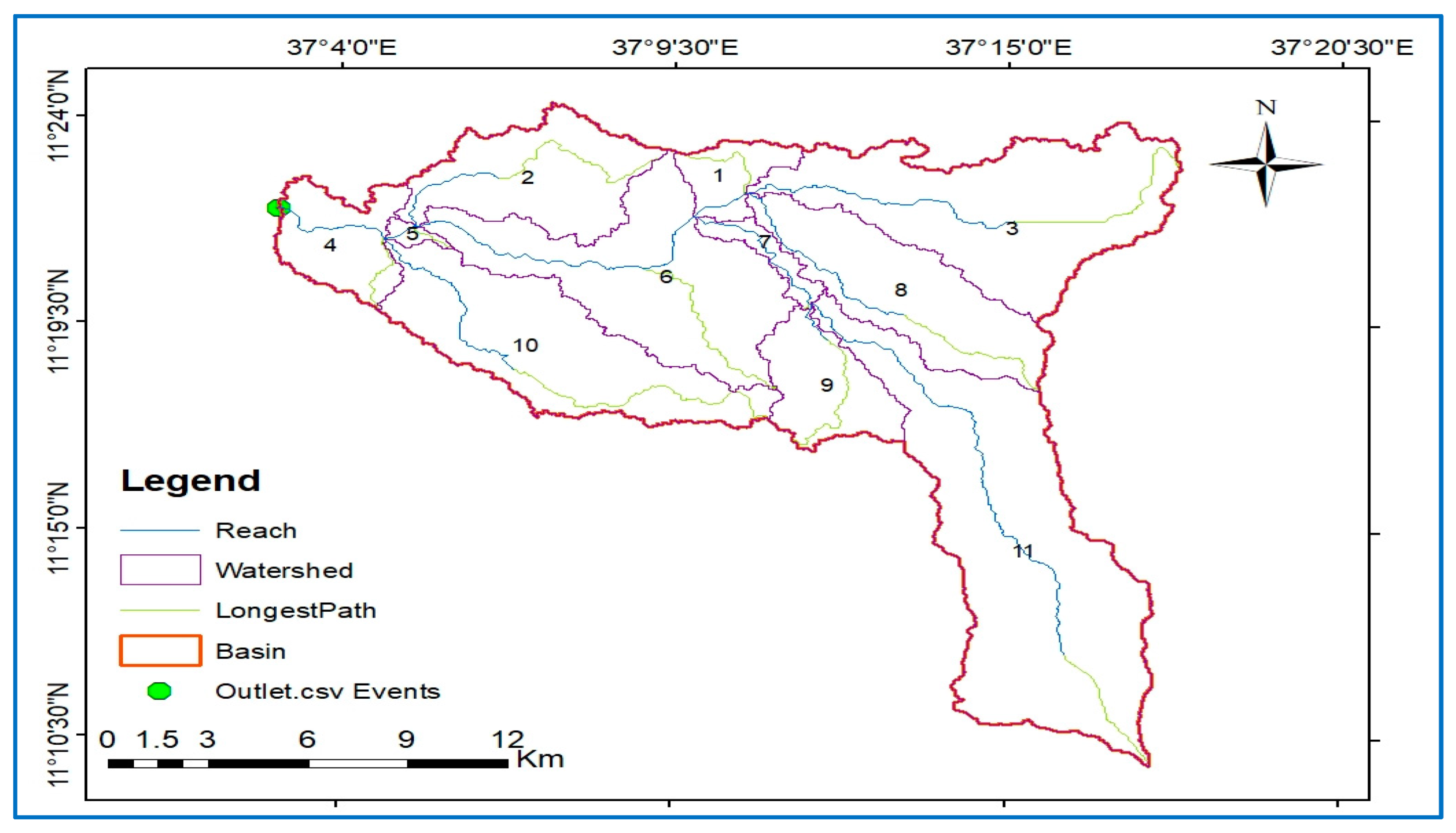
During the watershed delineation phase, the Koga River catchment was split into 11 sub-basins (Figure 2). The topographic components, such as the elevation (ranges from 1904 to 3092) and slope of the watershed, are specified during watershed delineation.
By dividing the watershed into regions with the same land use, soil, and slope combinations, it is possible to compare the differences in sediment yield and other hydrologic components for various land covers and soils. HRU definitions with several possibilities, which are taken into account for 1% threshold values for land use, 10% for soil, and 10% for slope, are employed in this study while simulating the hydrologic and sediment components.
2.6. Model Sensitivity Analysis, Calibration, and Validation
Sensitivity analysis is a method for identifying the model parameters that have the greatest impact on the result. By avoiding the parameters deemed to be insensitive, the objective is to reduce the number of parameters in the calibration procedure [66]. It is necessary to perform a sensitivity analysis, calibrate the model, and validate it before using the results of the model prediction directly for predicting the constituent streamflow and sediment output [66].
The SWAT CUP program uses two main sensitivity analysis techniques: one-at-a-time (OAT), or local sensitivity analysis, and all-at-once (AAT), or global sensitivity analysis. Of these, the global sensitivity analysis (AAT) type evaluation technique is used in this study. This is because this technique produces a more accurate result and works with the multiple regression techniques to determine the sensitivity of each parameter [66]. During the steps of sensitivity analysis, calibration, and validation, the semi-automated sequential uncertainty fitting (SUFI_2) is utilized. Because SUFI-2 is an iterative method, compared to PSO and generalized likelihood uncertainty estimation, it would not necessitate as many runs in each iteration (GLUE). In addition, it is useful in making the model result envelop most of the measurements well, and it encompasses the stochastic calibration. PSO and GLUE require too many numbers of iterations and simulations [66]. The parameters designated as the most sensitive during the sensitivity analysis are those with the highest absolute value of t-stat and the lowest p-value [66].
Fourteen of the eighteen flow parameters that underwent sensitivity analysis during the analysis are selected as the most sensitive parameters. Sixteen parameters that directly affect siltation and silt transport in the watershed are subjected to sensitivity analyses for sediment parameters. Based on their sensitivity rankings, the top ten sediment parameters are selected.
2.7. Model Performance Evaluation
3. Results and Discussion
3.1. Land Use/Cover Change Detection
The Koga River catchment’s land use and land cover change trend is evaluated during the years 1991–2018. Following systematic processing and land cover identification, the map for 1991, 2008, and 2018 only displayed seven classifications of land use/cover (Figure 3). The agricultural area, water body, grassland, bushland, built-up area, wetland, and forest area are the land use/cover classes available in the study area. Among these classes of LULC, the cultivated area covers the most abundant part of the catchment area. This implies that the life of the society living in the watershed was highly dependent on the cultivation activity.
3.2. Landsat Image Classification Accuracy Assessment
The accuracies of the classification in the land use and land cover maps of 1991, 2008, and 2018 are assessed with a confusion matrix using 480, 475, and 443 arbitrarily chosen control points, respectively. The maps’ overall accuracy and Kappa statistics both exceeded 85% during the accuracy testing. These figures imply that the overall classification and the method of classification used in this analysis were likewise accurate.
Overall accuracy: Overall accuracies of 93.56%, 93.60%, and 94.65% were achieved for the classified land use and land cover maps of 1991, 2008, and 2018, respectively. This value is in agreement with the minimum accuracy level (85%), as recommended by Ref [67].
Producer’s accuracy: The result of the producer’s accuracy for all the LULC maps was between 65.63% and 100%. The accuracy of the method is impacted by inaccurate classification because different land cover classes’ spectral values are comparable. For instance, a minimum procedure accuracy value (65.63%) was achieved for “Bushland”, and this value occurred due to the similar spectral properties of bushland with grassland and forest area.
User’s accuracy: The result of the user’s accuracy of the LULC maps ranges from 50% to 100%, as indicated in the table below. The minimum value achieved in the settlement area is, to some extent, incorrectly classified due to the similar spectral property of built-up area with cultivated land.
Kappa coefficient: The results of the Kappa statistics for the 1991, 2008, and 2018 maps are 0.90, 0.91, and 0.93, respectively. This implied that the classification and the method used were almost accurate based on the minimum fulfillment criteria recommended in Ref [56].
3.3. The Magnitude of Land Use/Cover Changes
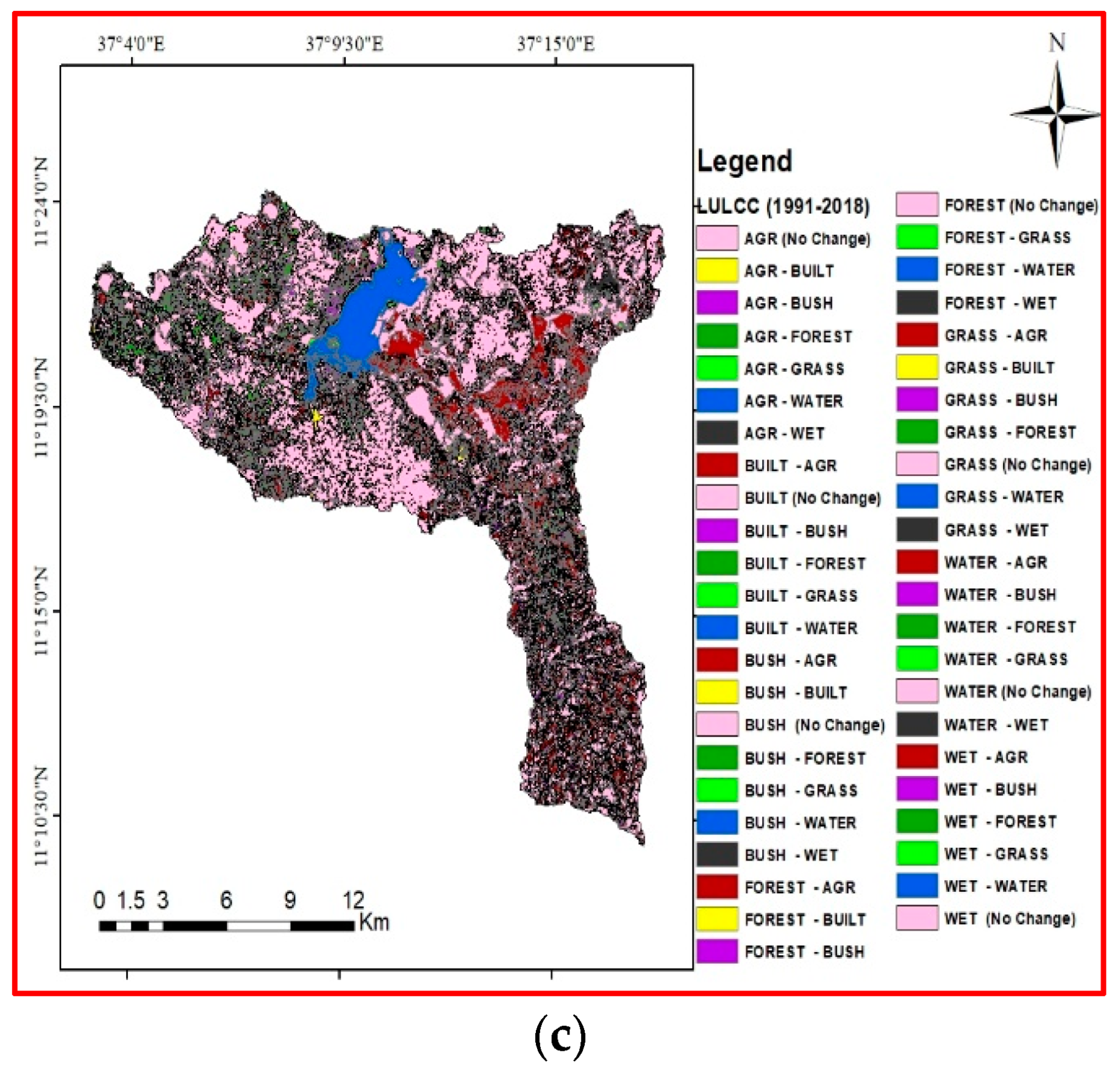
The land use and cover of the research area are clearly altered during the study period (Figure 4). The first study period (1991–2008) revealed a growing trend for the agricultural land, built-up area, forestland, water body, and wetland with 1.57%, 0.24%, 3.28%, 0.38%, and 1.35%, respectively. Meanwhile, grassland diminished by 4.52%, and the bush area was reduced by 2.30%. Similarly, in the second period (2008–2018), the agricultural land, built-up area, forestland, and water body increased by 12.64%, 0.15%, 3.08%, and 3.92%, respectively. On the contrary, grass area, bush area, and wetland diminished by 18.39%, 0.50%, and 0.89%, respectively (Figure 5 and Figure 6).
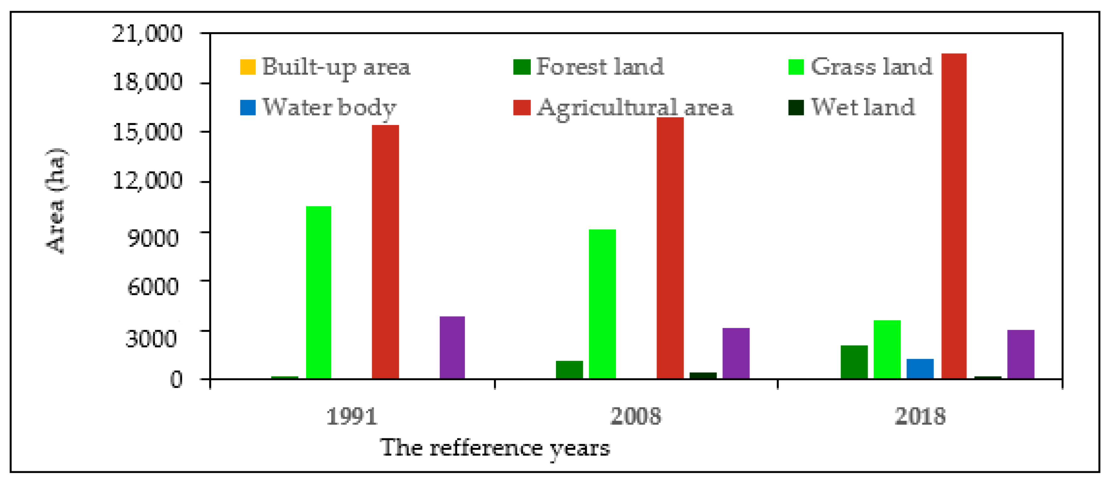
Throughout the study period, the major LULC modification occurred within the cultivated area and grass area. The area of cultivation expanded by 14.21%, and the grass area was reduced by 22.91%. Similar to this, due to the reforestation policy implemented during the Ethiopian millennium, forest area increased by 6.36%. The remaining LULC types (settlement area, water area, and wet area) expanded by 0.39%, 4.30%, and 0.46%, respectively. Contrarily, bushland decreased by 2.80%. These results implied that the modification in certain land use/cover types caused a decrease/increase in the other land use/cover types.
During the full study period, around 5132.17 ha of the grass area was converted to tillage land. Moreover, around 1139.67 hectares, 633.60 hectares, and 128.92 hectares of grassland were changed to water body, forestland, and wetland, respectively. Similarly, the wider context of bushland (around 2177.93 ha) was converted to cultivated land, and 1414.88 ha of bushland was changed into forest area.
The results generally implied that the watershed had clearly undergone LULC alteration over the previous 28 years. In this regard, the tendency points to a propensity for more land to be put to agricultural use. Thus, it is possible to say that the agricultural activity and built-up area were expanded at the expense of other LULC types (mainly grass and bushlands) to fulfill the needs of the drastically increased society in the watershed. In the watershed researched, forests (i.e., eucalyptus plantations) also gained importance and slightly expanded during the period of the study. In response to a dearth of fuel wood and other demands, a eucalyptus tree was planted in the watershed, which led to this outcome [68]. Due to the construction of the Koga dam in the watershed, the water body has significantly increased in size during the same time. On the other hand, the expansion of the agriculture area and the presence of the Koga dam, which were visible in the 2011 picture, have greatly reduced (down by 22.91%) the amount of grassland.
The watershed under study has a rapidly increasing population, similar to the rest of the nation [68]. It is anticipated that the study area’s natural resources will experience increased stress because of such unprecedented population growth. The major effects of changes in land use and land cover include soil erosion, land degradation, rural–urban migration, farmland fragmentation, climate change, and reduced crop yields [69]. Therefore, the implication of studying the impacts of land use and land cover change in a certain watershed is relevant for the decision makers in implimenting land management policies and governance practices [70].
Several studies on land use/cover change analyses were carried out in and around the Blue Nile Basin, especially in the Lake Tana sub-basin. Among these, Ref [35] assessed the changes in land use and cover in the Gilgel Abbay watershed and the Lake Tana sub-basin, and their findings were identical to those of this study. These researchers confirmed that there was an expansion of agricultural areas at the expense of bush and grasslands. Similarly, Ref [71] confirmed the result of this land use/cover study on the Gilgel Abbay watershed, as there was an increasing trend of cultivated land of 46% at the expense of other land use/covers. In the Koga watershed, Ref [68] evaluated the impact of changing land use and cover on watershed quality and concluded that there was an expansion of agricultural and forest area and a reduction in grassland and bushland. Hence, the results of Refs [68,71] were consistent with the findings of this study.
3.4. Sensitivity Analysis of the Flow and Sediment Yield Parameters
After pre-processing the required input for the SWAT_CUP software, simulations for a sensitivity analysis are performed using the thirteen years of flow data, starting from 1991 to 2003. Fourteen of the eighteen flow parameters that underwent sensitivity analysis are preferred as the most delicate parameters based on their p-value and t-statistic (Table 3). Similarly, a sensitivity analysis of the sediment parameters was undertaken using sixteen parameters that directly influence the siltation and silt transport in the watershed, and ten of them were determined as the most sensitive parameters (Table 4).
The SWAT Model Calibration and Validation
The task of calibration was performed with the parameters, which were determined as the most sensitive parameters. The parameter ranges used during calibration were directly applied for validation without further changes using an independently measured dataset.
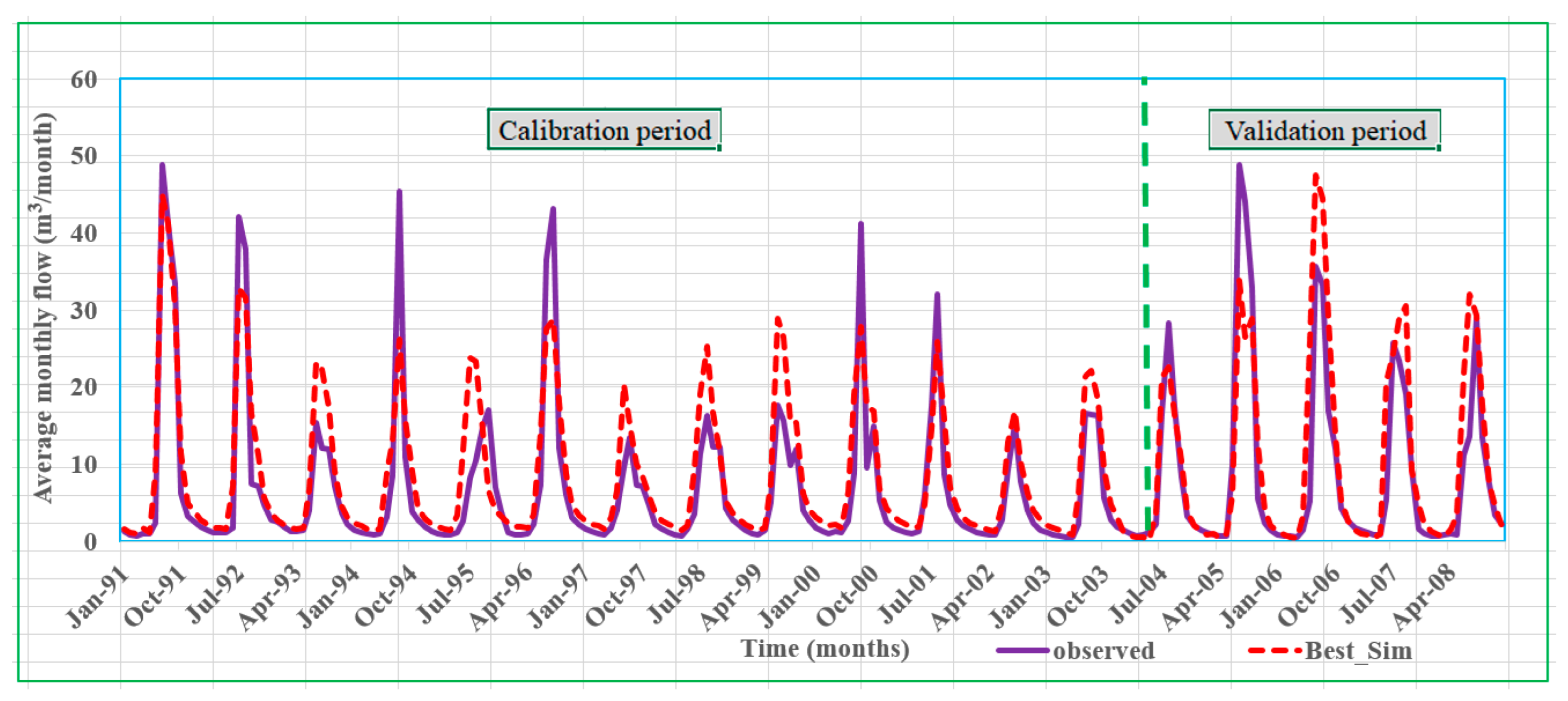
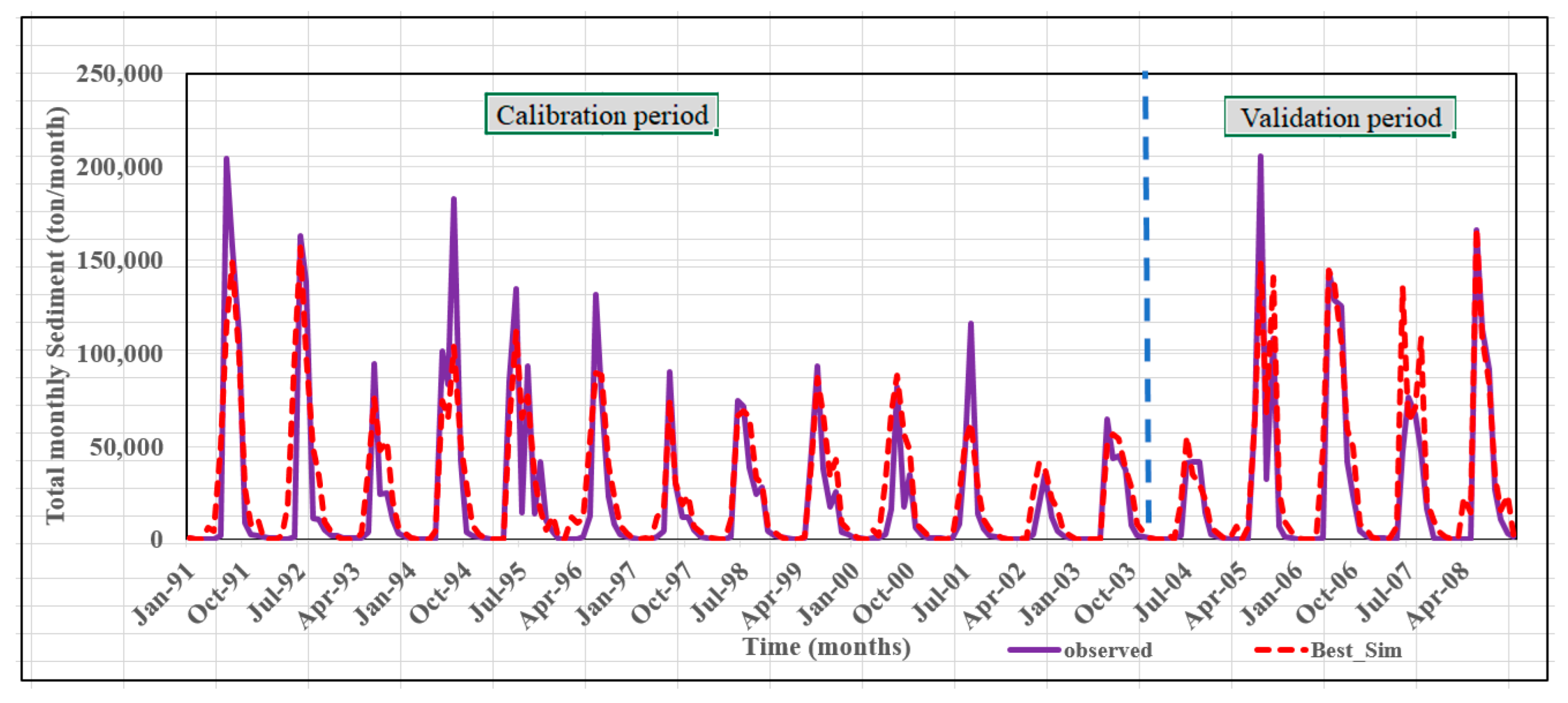
Utilizing the monthly observed data from the Merawi gauging station (outlet of the watershed), the flow and sediment yield calibration and validation are carried out. According to Ref [66], two-thirds of the river discharge and sediment data (1991–2003), excluding the three-year warm-up period, are utilized for calibration, and the remaining one-third (2004–2008) are utilized for validation. The evaluation parameters for measuring model efficiency are the coefficient of determination (R2), Nash–Sutcliffe efficiency (NSE), percent of bias (PBIAS), and RMSE observations–standard deviation ratio (RSR) (Table 5).
As indicated in the above Table 5, the measured and predicted data are in good agreement [23]. Hence, the model expresses the hydrological traits of the catchment at Merawi gauging station and may be used as a baseline for similar analysis. Finally, a month-to-month time setup of flow (Figure 7) and sediment output hydrograph (Figure 8) are formed to compare the recorded and simulated data.
3.5. The Effects of Land Use/Cover Change on the Streamflow
The dry season (from November to April), the rainy season (from May to October), and the average flow for the full year (from January to December) are used to analyze the change in streamflow caused by the change in land use and land cover (Table 6).
As indicated in the Table 6 above, in the years 1991 to 2008, the flow during the rainy months increased from 15.81 m3/s to 15.92 m3/s, and the flow decreased from 1.75 m3/s to 1.73 m3/s during the dry months. The mean monthly flow throughout the year (which is from January to December) also increasingly changed from 1991 to 2008. Hence, the increasing trend was from 8.78 m3/s to 8.83 m3/s. According to the analysis above, there was a 0.69% (0.11 m3/s) increase in the mean monthly streamflow during the wet months, and this change can be characterized as an increasing impact on the flow record due to the LULC changes in the catchment. The flow rate was, however, reduced by 0.95% (0.02 m3/s) during the dry season. This is because the shallow aquifer’s contribution to streamflow from groundwater that returns during the dry season was reduced. This finding showed that the LULC modification had a negative (declining) impact on the streamflow of the watershed during the research period’s dry season. In a similar fusion, the entire mean monthly streamflow (1991–2008) of the watershed increased by 0.57% (0.05 m3/s), and generally, the LULC alteration in the watershed implied an increasing impact on the discharge of the Koga river basin.
The increased streamflow is initiated by the excessive widening of agricultural activity in the watershed. This can be elaborated with the knowledge of crop and soil moisture needs. Crops require less soil moisture, and the storm provides sufficient water to saturate the soil in the cultivation land more quickly and releases more floods when the area under cultivation is wider. This idea is connected to the claim that the LULC type may predict both the infiltration and runoff aspects by monitoring how the storm events unfold [72]. While reducing infiltration lowers the base flow during the dry season, this lowers the amount of flow that can percolate to recharge the groundwater.
In general, the hydrological investigation’s response to the change in land use and cover within the Koga watershed indicated that the flow characteristics had changed (increased) because of the LULC change, which had taken place in the catchment.
Several studies were conducted in several watersheds of Ethiopia, specifically in the Blue Nile basin, to investigate the influences of LULC modification on streamflow. Among these, a modeling study of the Gilgel Abbay watershed by Ref [71] revealed that the streamflow increased as a result of the expansion of agricultural land in the watershed. Similarly, Ref [73], studying the Anger watershed in Ethiopia, stated that the flow increased from year to year because of the increase in agricultural land; this study was in agreement with those studies, as the flow in the Koga watershed increased due to the increase in agricultural land from year to year.
3.6. Land Use/Cover Change Effects on the Sediment Yield
The effect of land use/cover change on the watershed’s sediment production is measured using the two different land use/cover maps. Due to changes in land use and cover, the annual sediment production of the Koga watershed has marginally grown from year to year (Table 7).
Based on the results above (Table 7), the amount of average sediment yield per year had increased. An increase in the agricultural area (1991–2008) of 1.57% was a vital factor in the increase in siltation of 0.08 t/ha/yr. Although most of the supplying sub-catchments are significantly erodible and result in much of the coarse sediments, the sediment yield and the change in the sediment yield from year to year are relatively low. This may be due to the implementation of soil and water conservation strategies, such as check dams, terraces, cut-off drains, and canals, imposed on the watershed by the Rural Development Bureau, as stated by Ref [40]. On the other hand, during the years 1991–2008, there was a high level of afforestation, and thus, the forest area increased by 3.28% in the watershed. Moreover, among the watershed’s primary soil types, 33.76% of the soil cover consists mainly of vertisols. Vertisols are strong enough to resist detachment from the surface, since they are highly cohesive. Because of the aforementioned factors, the sediment production of the watershed in the two simulation years was within the acceptable range of soil loss levels for Ethiopia’s agro-ecological zones, which is from 2 t/ha/yr to 18 t/ha/yr, as stated by Ref [74].
These changes in the sediment yield implied that land use modification has a tangible effect on the siltation of the Koga watershed. In addition to the increased trend of cultivated land (generating more surface runoff), there was a decrease in grassland and shrub land, which ultimately led to an increase in sediment output. The soil layer was loosened by cultivation activity, which eventually allowed the soil layer to pass through water with ease, especially during times of high flow. This is because the sediment movement has a direct correlation with the river flow occurring in the watershed. In general, the change in cultivated land showed a proportional linkage with sediment yield. Meanwhile, grassland and shrub land showed an inverse relation with sedimentation in the watershed under study. Thus, it can be declared that the alteration in the LULC had an impact on the sediment regime of the Koga river basin (increased sediment yield) in the years 1991 to 2008.
This study has an equivalent result to the previous studies in the watershed. For instance, Refs [40,47,75] estimated the sediment output of the watershed and achieved a yield approximate to this study. Their outcomes were within the acceptable soil loss range of Ethiopia’s different agricultural and ecological environments.
3.7. The Spatial Distribution of Sediments in the Watershed
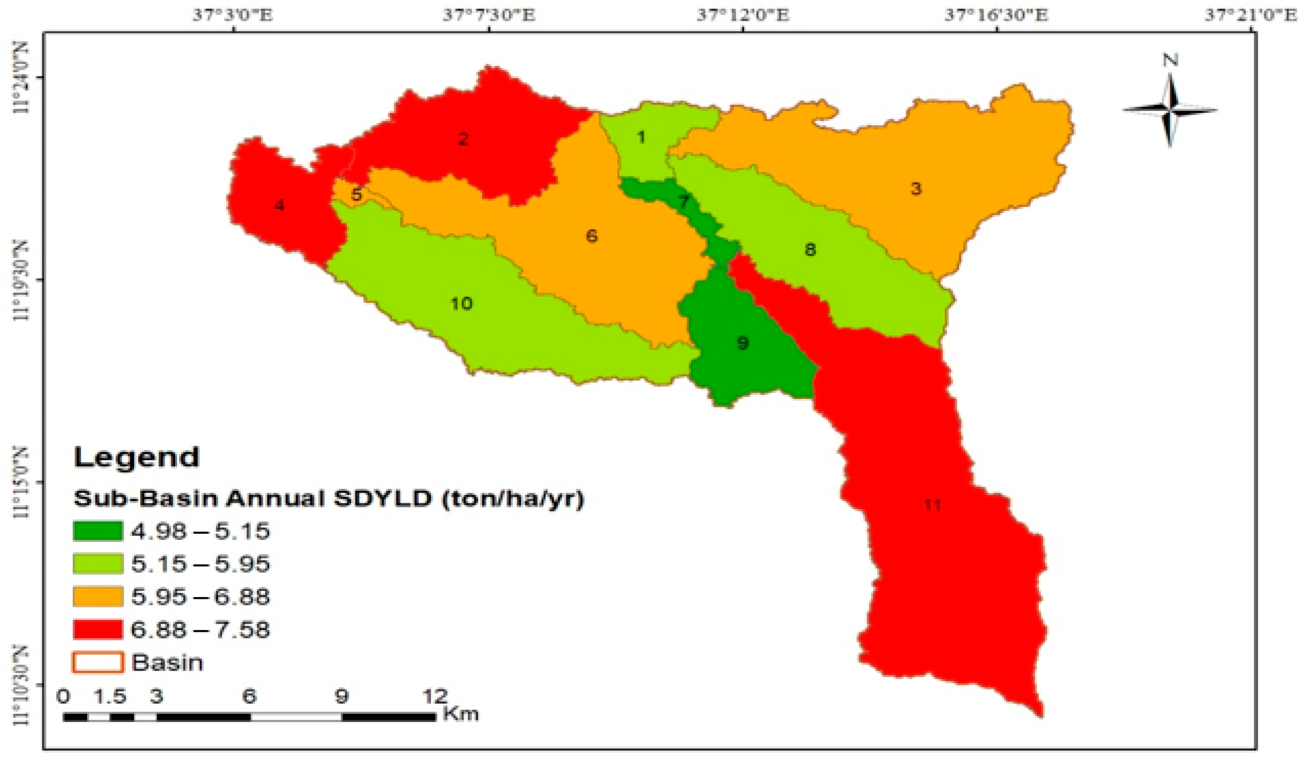
The Koga watershed’s spatial variation in sediment yield is identified from the validated sediment outputs. Analyzing the sediment variability of a watershed is also useful for identifying the potential erosion hotspot areas and applying watershed management measures within the erosion-severe areas to avoid siltation of the catchment. In order to identify which region has a high/low silt supply, the graphic below (Figure 9) shows the spatial visualization of sub-basin sediment yield in t/ha/yr.
After the model simulation phase, the areal distribution of sediment in each sub-basin of the Koga catchment is executed. Some downstream and upstream parts of the area were exposed to comparatively high erosion (Figure 9). This is due to the reason that the area is of a hilly and mountainous nature. The levels of soil erosion or sedimentation in the sub-basins are categorized in order to understand the distribution of sediments in the watershed. The categories are: very low (from 0 to 5 t/ha/yr), low (from 5 to 11 t/ha/yr), moderate (from 11 to 18 t/ha/yr), high (from 18 to 25 t/ha/yr), and very high (greater than 25 t/ha/yr). This category is based on the classification of Ref [76] applied near the study area.
The sediment output of each sub-basin is categorized into extremely low and low stages of sedimentation based on the sediment results of each sub-basin in the Koga watershed shown in the figure and table above (Table 8). Sub-basins 2, 4, and 11 are those with the highest yearly sediment generation; these sub-watersheds are interpreted as the highest sources of sediment in the watershed. All these sub-catchments have annual sediment distribution ranges from 6.88 tons/hectare/year to 7.58 tons/hectare/year. Additionally, sub-catchments 1, 7, 8, 9, and 10 in the research area have the lowest annual sediment generation, with year-to-year sediment output ranging from 4.98 to 5.95 t/ha/yr. The remaining sub-basins (3 and 6) generate an annual sediment yield ranging from 5.95 t/ha/yr to 6.88 t/ha/yr.
Refs [40,77] anticipated the sediment yield and reservoir siltation in highly dynamic regions, as in the case of the Koga reservoir in Ethiopia. This research declared that the predicted soil loss rate ranged from 0.10 t/ha/yr to 3.55 t/ha/yr. Similarly, Ref [76] examined the performance of the best management strategies in soil erosion minimization in the case of the Gumara watershed in the Abbay (Upper Blue Nile) basin. This study revealed that the sediment yield sourced from each sub-area of the watershed was between 0 and 38 t/ha/yr. Ref [40] achieved a yield approximate to this study. The sediment yields for sub-catchments in this investigation, however, were distinct from those in Ref [77]. This may be due to the combined effect of soil and water management structures implemented in the Koga watershed and the watershed characteristics, such as land use, soil type, and slope distribution.
3.8. Seasonal Variation of Sediment Yield in the Watershed
The catchment area, land use, soil type, slope, and climate all affect catchment siltation. After the model simulation for the flow and sediment regimes, the relationship among siltation, catchment runoff, and precipitation showed a direct linkage, whereby higher rainfall would result in higher runoff and sediment yield. As a result, a high sediment yield was observed in June, July, August, and September (Table 9). This occurred due to high/peak runoff occurring during these months, thereby leading to a higher rate of soil erosion. On the other hand, dry seasons with very little flow had a very low rate of soil erosion (sediment movement).
The amount of silt produced by the watershed grew year to year due to the tendency of cultivated land extension in the study area; the seasonal change of sediment became highly vivid. The mean monthly sediment load carried by the Koga River was computed as 0.17 t/ha. This result is similar to the result computed by Ref [75]. The figure below shows the seasonal fluctuation of sediment in the sub-basins under the Koga watershed.
A previous study by Ref [35] determined that there was a high seasonal variation of sediment in the Gilgel Abbay watershed in the Abbay basin, more specifically in the Gilgel Abbay watershed, after assessing the seasonal variation of sediment yield in the catchment. Similar to this study, large amounts of silt were produced in June, July, August, and September in the prior study.
4. Conclusions
This study aimed to assess the dynamics of changes in the land use/cover of the Koga watershed from 1991 to 2018 using the supervised image classification approach. From the analysis of land use/cover change, it can be summarized that the watershed under study had undergone a meaningful spatial and temporal change in land use/cover. In the years 1991 to 2018, the area of cultivation expanded by 14.21%, and the grass area was reduced by 22.91%. The remaining LULC types (settlement area, water area, and wet area) expanded by 0.39%, 4.30%, and 0.46%, respectively. Contrarily, bushland decreased by 2.80%. During the study period, most parts of the grass area were converted to a cultivation area, water body, and forest cover. Meanwhile, the abundant coverage of bushland was converted to a cultivation area and forest area. Even though the agricultural area increased significantly, 1246.42 hectares of the area was changed into forestland throughout the study period. This result showed that there was a significant LULC change in the Koga watershed from 1991 to 2008. Reduced crop yields, soil erosion, land degradation, rural–urban migration, farmland fragmentation, climate change, and land degradation are all significant repercussions of the changes in land use and land cover. The decision makers who implement land management policies and governance practices should therefore consider the implications of assessing the effects of changing land use and land cover in a particular watershed.
After effective model calibration and validation, the impact of land use/cover change on the streamflow and sediment yield was assessed. During the years 1991–2008, a significant change within the streamflow occurred both in the wet and dry periods. Hence, the flow rate in the dry months was reduced by 0.95% (0.02 m3/s), while the flow during the wet months increased by 0.76% (0.11 m3/s). The entire mean monthly streamflow (1991–2008) of the watershed increased by 0.57% (0.05 m3/s), and generally, the LULC alteration in the watershed implied an increasing impact on the discharge of the Koga river basin. Similarly, the sediment yield increased from 1991 to 2008 by 0.08 t/ha/yr due to the conversion of bushland and grassland into a cultivation area. This result implied that there was a change in the flow and sedimentation regime of the watershed due to the change in the LULC of the watershed.
The watershed’s areal and seasonal variations in sediment were assessed, and the significant sources of excess sediment were identified. As a result, the sub-watersheds generated an annual sediment yield ranging from 4.98 t/ha/yr to 7.58 t/ha/yr. In June, July, August, and September, there was a substantial amount of sediment.
Author Contributions
Conceptualization, H.A.A.; methodology; software; validation, H.A.A., L.B., T.W.W. and A.O.A.; formal analysis, H.A.A.; investigation, H.A.A.; resources, H.A.A.; data curation, H.A.A.; writing—original draft preparation, H.A.A.; writing—review and editing, A.O.A. and L.B.; visualization, A.O.A. and L.B.; supervision, T.W.W., A.O.A. and L.B.; project administration, H.A.A. and T.W.W.; funding acquisition, H.A.A. All authors have read and agreed to the published version of the manuscript.
Funding
This research was funded by the Bule Hora University College of engineering and Technology post graduate Research Project Fund.
Data Availability Statement
Data can be provided upon request.
Acknowledgments
We would like to thank the Ethiopian Ministry of Water and Energy (MoWE) and National Meteorological Agency (NMA) for providing the streamflow, sediment data, and climate data.
Conflicts of Interest
The authors declare that they have no conflict of interest.
References
- Kılıç, Z. The Importance of Water and Conscious Use of Water. Int. J. Hydrol. 2020, 4, 239–241. [Google Scholar] [CrossRef]
- Nigussie, A. Impact of Land Use Land Cover Change on Stream Flow (CASE STUDY GILGEL GIBE III). Master’s Thesis, Addis Ababa Institute of Technology, Addis Ababa, Ethiopia, 2007. [Google Scholar]
- Bogale, A. Review, Impact of Land Use/Cover Change on Soil Erosion in the Lake Tana Basin, Upper Blue Nile, Ethiopia. Appl. Water Sci. 2020, 10, 235. [Google Scholar] [CrossRef]
- Wang, J.; Sui, L.; Yang, X.; Wang, Z.; Ge, D.; Kang, J.; Yang, F.; Liu, Y.; Liu, B. Economic Globalization Impacts on the Ecological Environment of Inland Developing Countries: A Case Study of Laos from the Perspective of the Land Use/Cover Change. Sustainability 2019, 11, 3940. [Google Scholar] [CrossRef] [Green Version]
- Mango, L.M.; Melesse, A.M.; McClain, M.E.; Gann, D.; Setegn, S.G. Land Use and Climate Change Impacts on the Hydrology of the Upper Mara River Basin, Kenya: Results of a Modeling Study to Support Better Resource Management. Hydrol. Earth Syst. Sci. 2011, 15, 2245–2258. [Google Scholar] [CrossRef] [Green Version]
- Nyatuame, M.; Amekudzi, L.K.; Agodzo, S.K. Assessing the Land Use/Land Cover and Climate Change Impact on Water Balance on Tordzie Watershed. Remote Sens. Appl. Soc. Environ. 2020, 20, 100381. [Google Scholar] [CrossRef]
- Molina, A.; Vanacker, V.; Balthazar, V.; Mora, D.; Govers, G. Complex Land Cover Change, Water and Sediment Yield in a Degraded Andean Environment. J. Hydrol. 2012, 472–473, 25–35. [Google Scholar] [CrossRef]
- Aghsaei, H.; Mobarghaee Dinan, N.; Moridi, A.; Asadolahi, Z.; Delavar, M.; Fohrer, N.; Wagner, P.D. Effects of Dynamic Land Use/Land Cover Change on Water Resources and Sediment Yield in the Anzali Wetland Catchment, Gilan, Iran. Sci. Total Environ. 2020, 712, 136449. [Google Scholar] [CrossRef]
- Kefay, T.; Abdisa, T.; Chelkeba Tumsa, B. Prioritization of Susceptible Watershed to Sediment Yield and Evaluation of Best Management Practice: A Case Study of Awata River, Southern Ethiopia. Appl. Environ. Soil Sci. 2022, 2022, e1460945. [Google Scholar] [CrossRef]
- Dechasa, A.; Aga, A.O.; Dufera, T. Erosion Risk Assessment for Prioritization of Conservation Measures in the Watershed of Genale Dawa-3 Hydropower Dam, Ethiopia. Quaternary 2022, 5, 39. [Google Scholar] [CrossRef]
- Kenea, U.; Adeba, D.; Regasa, M.S.; Nones, M. Hydrological Responses to Land Use Land Cover Changes in the Fincha’a Watershed, Ethiopia. Land 2021, 10, 916. [Google Scholar] [CrossRef]
- Tolessa, T.; Senbeta, F.; Kidane, M. The Impact of Land Use/Land Cover Change on Ecosystem Services in the Central Highlands of Ethiopia. Ecosyst. Serv. 2017, 23, 47–54. [Google Scholar] [CrossRef]
- Sibanda, S.; Ahmed, F. Modelling Historic and Future Land Use/Land Cover Changes and Their Impact on Wetland Area in Shashe Sub-Catchment, Zimbabwe. Model. Earth Syst. Environ. 2021, 7, 57–70. [Google Scholar] [CrossRef]
- Mishra, V.; Rai, P.; Mohan, K. Prediction of Land Use Changes Based on Land Change Modeler (LCM) Using Remote Sensing: A Case Study of Muzaffarpur (Bihar), India. J. Geogr. Inst. Jovan Cvijic SASA 2014, 64, 111–127. [Google Scholar] [CrossRef]
- Mahamud, M.A.; Samat, N.; Tan, M.L.; Chan, N.W.; Tew, Y.L. Prediction Of Future Land Use Land Cover Changes Of Kelantan, Malaysia. ISPRS Int. Arch. Photogramm. Remote Sens. Spat. Inf. Sci. 2019, XLII-4/W16, 379. [Google Scholar] [CrossRef] [Green Version]
- Getahun, Y.S.; HAJ, V.L. Assessing the Impacts of Land Use-Cover Change on Hydrology of Melka Kuntrie Subbasin in Ethiopia, Using a Conceptual Hydrological Model. J. Waste Water Treat. Anal. 2015, 6, 1000210. [Google Scholar] [CrossRef] [Green Version]
- Hailemariam, S.N.; Soromessa, T.; Teketay, D. Land Use and Land Cover Change in the Bale Mountain Eco-Region of Ethiopia during 1985 to 2015. Land 2016, 5, 41. [Google Scholar] [CrossRef] [Green Version]
- Bekele, M. The Ethiopian Forest from Ancient Time to 1900: A Brief Account. Walia 1989, 1998, 3–9. [Google Scholar]
- Angassa, A. Effects of Grazing Intensity and Bush Encroachment on Herbaceous Species and Rangeland Condition in Southern Ethiopia. Land Degrad. Dev. 2014, 25, 438–451. [Google Scholar] [CrossRef]
- Rientjes, T.H.M.; Haile, A.T.; Kebede, E.; Mannaerts, C.M.M.; Habib, E.; Steenhuis, T.S. Changes in Land Cover, Rainfall and Stream Flow in Upper Gilgel Abbay Catchment, Blue Nile Basin—Ethiopia. Hydrol. Earth Syst. Sci. 2011, 15, 1979–1989. [Google Scholar] [CrossRef] [Green Version]
- Kidane, D.; Alemu, B. The Effect of Upstream Land Use Practices on Soil Erosion and Sedimentation in the Upper Blue Nile Basin, Ethiopia. Res. J. Agric. Environ. Manag. 2015, 4, 55–68. [Google Scholar] [CrossRef]
- Nyssen, J.; Poesen, J.; Moeyersons, J.; Deckers, J.; Haile, M.; Lang, A. Human Impact on the Environment in the Ethiopian and Eritrean Highlands—A State of the Art. Earth-Sci. Rev. 2004, 64, 273–320. [Google Scholar] [CrossRef]
- Endalamaw, N.T.; Moges, M.A.; Kebede, Y.S.; Alehegn, B.M.; Sinshaw, B.G. Potential Soil Loss Estimation for Conservation Planning, Upper Blue Nile Basin, Ethiopia. Environ. Chall. 2021, 5, 100224. [Google Scholar] [CrossRef]
- Yang, D.; Kanae, S.; Oki, T.; Koike, T.; Musiake, K. Global Potential Soil Erosion with Reference to Land Use and Climate Changes. Hydrol. Process. 2003, 17, 2913–2928. [Google Scholar] [CrossRef]
- Alemayehu, K.; Sheleme, B.; Schoenau, J. Characterization of Problem Soils in and around the South Central Ethiopian Rift Valley. J. Soil Sci. Environ. Manag. 2016, 7, 191–203. [Google Scholar] [CrossRef] [Green Version]
- Belayneh, L.; Dewitte, O.; Gulie, G.; Poesen, J.; O’Hara, D.; Kassaye, A.; Endale, T.; Kervyn, M. Landslides and Gullies Interact as Sources of Lake Sediments in a Rifting Context: Insights from a Highly Degraded Mountain Environment. Geosciences 2022, 12, 274. [Google Scholar] [CrossRef]
- Belayneh, L.; Bantider, A.; Moges, A. Road Construction and Gully Development in Hadero Tunto—Durgi Road Project, Southern Ethiopia. Ethiop. J. Environ. Stud. Manag. 2014, 7, 720–730. [Google Scholar] [CrossRef]
- Karnez, E.; Sagir, H.; Gavan, M.; SaidGolpinar, M.; Cetin, M.; Akgul, M.A.; Ibrikci, H.; Pintar, M. Modeling Agricultural Land Management to Improve Understanding of Nitrogen Leaching in an Irrigated Mediterranean Area in Southern Turkey; IntechOpen: London, UK, 2017; ISBN 978-953-51-2882-3. [Google Scholar]
- Dananto, M.; Aga, A.O.; Yohannes, P.; Shura, L. Assessing the Water-Resources Potential and Soil Erosion Hotspot Areas for Sustainable Land Management in the Gidabo Watershed, Rift Valley Lake Basin of Ethiopia. Sustainability 2022, 14, 5262. [Google Scholar] [CrossRef]
- Aga, A.O.; Melesse, A.M.; CHANE, B. An Alternative Empirical Model to Estimate Watershed Sediment Yield Based on Hydrology and Geomorphology of the Basin in Data-Scarce Rift Valley Lake Regions, Ethiopia. Geosciences 2020, 10, 31. [Google Scholar] [CrossRef] [Green Version]
- Aga, A.O.; Melesse, A.M.; Chane, B. Estimating the Sediment Flux and Budget for a Data Limited Rift Valley Lake in Ethiopia. Hydrology 2019, 6, 1. [Google Scholar] [CrossRef] [Green Version]
- Aliye, M.A.; Aga, A.O.; Tadesse, T.; Yohannes, P. Evaluating the Performance of HEC-HMS and SWAT Hydrological Models in Simulating the Rainfall-Runoff Process for Data Scarce Region of Ethiopian Rift Valley Lake Basin. OJMH 2020, 10, 105–122. [Google Scholar] [CrossRef]
- Aga, A.O. Modeling Sediment Yield, Transport and Deposition in The Data Scarce Region of Ethiopian Rift Valley Lake Basin. Ph.D. Dissertation, Addis Ababa Institute of Technology, Addis Ababa, Ethiopia, 2019. [Google Scholar]
- Aga, A.O.; Chane, B.; Melesse, A.M. Soil Erosion Modelling and Risk Assessment in Data Scarce Rift Valley Lake Regions, Ethiopia. Water 2018, 10, 1684. [Google Scholar] [CrossRef]
- Andualem, T.G.; Gebremariam, B. Impact Of Land Use Land Cover Change On Stream Flow And Sediment Yield: A Case Study Of Gilgel Abay Watershed, Lake Tana Sub-Basin, Ethiopia. Int. J. Technol. Enhanc. Emerg. Eng. Res. 2015, 3, 28. [Google Scholar]
- Bekele, T. Effect of Land Use and Land Cover Changes on Soil Erosion in Ethiopia. Int. J. Agric. Sci. Food Technol. 2019, 5, 26–34. [Google Scholar] [CrossRef] [Green Version]
- McColl, C.; Aggett, G. Land-Use Forecasting and Hydrologic Model Integration for Improved Land-Use Decision Support. J. Environ. Manag. 2007, 84, 494–512. [Google Scholar] [CrossRef] [PubMed]
- Lemma, E. Sedimentation Problem and Mitigation Measure of Koga Reservoir. Master’s Thesis, Addis Ababa University, Addis Ababa, Ethiopia, 2018. [Google Scholar]
- Assefa, T.T.; Jha, M.K.; Tilahun, S.A.; Yetbarek, E.; Adem, A.A.; Wale, A. Identification of Erosion Hotspot Area Using GIS and MCE Technique for Koga Watershed in the Upper Blue Nile Basin, Ethiopia. Am. J. Environ. Sci. 2015, 11, 245–255. [Google Scholar] [CrossRef] [Green Version]
- Ayele, G.T.; Kuriqi, A.; Jemberrie, M.A.; Saia, S.M.; Seka, A.M.; Teshale, E.Z.; Daba, M.H.; Ahmad Bhat, S.; Demissie, S.S.; Jeong, J.; et al. Sediment Yield and Reservoir Sedimentation in Highly Dynamic Watersheds: The Case of Koga Reservoir, Ethiopia. Water 2021, 13, 3374. [Google Scholar] [CrossRef]
- Andualem, Y. Water Delivery Performance Evaluation of Koga Irrigation Scheme. Master’s Thesis, Addis Ababa University, Addis Ababa, Ethiopia, 2018. [Google Scholar]
- Tewabe, D.; Dessie, M. Enhancing Water Productivity of Different Field Crops Using Deficit Irrigation in the Koga Irrigation Project, Blue Nile Basin, Ethiopia. Cogent Food Agric. 2020, 6, 1757226. [Google Scholar] [CrossRef]
- Ran, L.; Lu, X.X.; Xin, Z.; Yang, X. Cumulative Sediment Trapping by Reservoirs in Large River Basins: A Case Study of the Yellow River Basin. Glob. Planet. Chang. 2013, 100, 308–319. [Google Scholar] [CrossRef]
- Cunderlik, M.J. Hydrologic Model Selection Fort the CFCAS Project: Assessment of Water Resources Risk and Vulnerability to Changing Climatic Conditions. In Project Report I By University of Western Ontario; University of Waterloo and Upper Thames River Conservation Authority: Waterloo, ON, Canada, 2003. [Google Scholar]
- Neitsch, S.L.; Arnold, J.G.; Kiniry, J.R.; Williams, J.R. Soil and Water Assessment Tool Theoretical Documentation Version 2009; Texas Water Resources Institute: College Station, TX, USA, 2009. [Google Scholar]
- Engel, B.A.; Srinivasan, R.; Arnold, J.; Rewerts, C.; Brown, S.J. Nonpoint Source (NPS) Pollution Modeling Using Models Integrated with Geographic Information Systems (GIS). Water Sci. Technol. 1993, 28, 685–690. [Google Scholar] [CrossRef]
- Mulatu, C.A. Analysis of Reservoir Sedimentation Process Using Empirical and Mathematical Method: Case Study—Koga Irrigation and Watershed Management Project; Ethiopia. Main 2015, 5, 1–13. [Google Scholar]
- Wilkinson, G.G.; Kanellopoulos, I.; Liu, Z.K.; Folving, S. Integrated Land-Cover Mapping from Satellite Imagery Using Artificial Neural Networks. Ground Sens. 1993, 1941, 68–75. [Google Scholar] [CrossRef]
- Abburu, S.; Babu Golla, S. Satellite Image Classification Methods and Techniques: A Review. Int. J. Comput. Appl. 2015, 119, 20–25. [Google Scholar] [CrossRef]
- Gashaw, T.; Tulu, T.; Argaw, M.; Worqlul, A.W. Evaluation and Prediction of Land Use/Land Cover Changes in the Andassa Watershed, Blue Nile Basin, Ethiopia. Environ. Syst. Res. 2017, 6, 17. [Google Scholar] [CrossRef]
- Dibs, H.; Hasab, H.A.; Al-Rifaie, J.K.; Al-Ansari, N. An Optimal Approach for Land-Use/Land-Cover Mapping by Integration and Fusion of Multispectral Landsat OLI Images: Case Study in Baghdad, Iraq. Water Air Soil Pollut. 2020, 231, 488. [Google Scholar] [CrossRef]
- Kassa, H.; Dondeyne, S.; Poesen, J.; Frankl, A.; Nyssen, J. Transition from Forest-Based to Cereal-Based Agricultural Systems: A Review of the Drivers of Land Use Change and Degradation in Southwest Ethiopia. Land Degrad. Dev. 2017, 28, 431–449. [Google Scholar] [CrossRef] [Green Version]
- Gashaw, T.; Bantider, A.; Mahari, A. Evaluations of Land Use/Land Cover Changes and Land Degradation in Dera District, Ethiopia: GIS and Remote Sensing Based Analysis. Int. J. Sci. Res. Environ. Sci. 2014, 2, 199–208. [Google Scholar] [CrossRef]
- Abbas, Z.; Jaber, H.S. Accuracy Assessment of Supervised Classification Methods for Extraction Land Use Maps Using Remote Sensing and GIS Techniques. IOP Conf. Ser. Mater. Sci. Eng. 2020, 745, 012166. [Google Scholar] [CrossRef]
- Manandhar, R.; Odehi, I.O.A.; Ancevt, T. Improving the Accuracy of Land Use and Land Cover Classification of Landsat Data Using Post-Classification Enhancement. Remote Sens. 2009, 1, 330–344. [Google Scholar] [CrossRef] [Green Version]
- Monserud, R.A.; Leemans, R. Comparing Global Vegetation Maps with the Kappa Statistic. Ecol. Model. 1992, 62, 275–293. [Google Scholar] [CrossRef]
- Grubbs, F.E. Procedures for Detecting Outlying Observations in Samples. Technometrics 1969, 11, 1–21. [Google Scholar] [CrossRef]
- Arnold, J.G.; Srinivasan, R.; Muttiah, R.S.; Williams, J.R. Large Area Hydrologic Modeling and Assessment Part I: Model Development. J. Am. Water Resour. Assoc. 1998, 34, 73–89. [Google Scholar] [CrossRef]
- Orkodjo, T.P. Impact of Land Use/Land Cover Change on Catchment Hydrology (A Case Study of Awassa Catchment) by : Impact of Land Use/Land Cover Change on Catchment Hydrology (A Case Study of Awassa Catchment). Master’s Thesis, Arba Minch University, Arba Minch, Ethiopia, 2014. [Google Scholar]
- Geremew, A.A. Assessing the Impacts of Land Use and Land Cover Change on Hydrology of Watershed: A Case Study on Gilgel—Abbay Watershed, Lake Tana, Ethiopia. Master’s Thesis, Jaume I University, Castelló de la Plana, Spain, 2013. [Google Scholar]
- Sith, R.; Nadaoka, K. Comparison of SWAT and GSSHA for High Time Resolution Prediction of Stream Flow and Sediment Concentration in a Small Agricultural Watershed. Hydrology 2017, 4, 27. [Google Scholar] [CrossRef] [Green Version]
- Polanco, E.I.; Fleifle, A.; Ludwig, R.; Disse, M. Improving SWAT Model Performance in the Upper Blue Nile River Basin Using Meteorological Data Integration and Catchment Scaling. Hydrol. Earth Syst. Sci. Discuss. 2017, 21, 4907–4926. [Google Scholar] [CrossRef]
- Shi, P.; Ma, X.; Hou, Y.; Li, Q.; Zhang, Z.; Qu, S.; Chen, C.; Cai, T.; Fang, X. Effects of Land-Use and Climate Change on Hydrological Processes in the Upstream of Huai River, China. Water Resour. Manag. 2013, 27, 1263–1278. [Google Scholar] [CrossRef]
- Xie, X.; Cui, Y. Development and Test of SWAT for Modeling Hydrological Processes in Irrigation Districts with Paddy Rice. J. Hydrol. 2011, 396, 61–71. [Google Scholar] [CrossRef]
- Arekhi, S.; Shabani, A.; Rostamizad, G. Application of the Modified Universal Soil Loss Equation (MUSLE) in Prediction of Sediment Yield (Case Study: Kengir Watershed, Iran). Arab. J. Geosci. 2012, 5, 1259–1267. [Google Scholar] [CrossRef]
- Abbaspour, K.C.; Vaghefi, S.A.; Srinivasan, R. A Guideline for Successful Calibration and Uncertainty Analysis for Soil and Water Assessment: A Review of Papers from the 2016 International SWAT Conference. Water 2017, 10, 6. [Google Scholar] [CrossRef] [Green Version]
- Shao, G.; Wu, J. The Accuracy of Landscape Pattern Analysis Using Remote Sensing Data. Landsc. Ecol. 2008, 23, 505–511. [Google Scholar] [CrossRef]
- Sewnet, A.; Abebe, G. Land Use and Land Cover Change and Implication to Watershed Degradation by Using GIS and Remote Sensing in the Koga Watershed, North Western Ethiopia. Earth Sci. Inform. 2018, 11, 99–108. [Google Scholar] [CrossRef]
- Agidew, A.A.; Singh, K.N. The Implications of Land Use and Land Cover Changes for Rural Household Food Insecurity in the Northeastern Highlands of Ethiopia: The Case of the Teleyayen Sub-Watershed. Agric. Food Secur. 2017, 6, 56. [Google Scholar] [CrossRef]
- Getu Engida, T.; Nigussie, T.A.; Aneseyee, A.B.; Barnabas, J. Land Use/Land Cover Change Impact on Hydrological Process in the Upper Baro Basin, Ethiopia. Appl. Environ. Soil Sci. 2021, 2021, e6617541. [Google Scholar] [CrossRef]
- Abuhay, W. Modeling the Impacts of Land Use/Land Cover Changes on the Hydrological Processes of Upper Gilgel Abay Watershed, Abbay River Basin, Ethiopia. Master’s Thesis, Bahir Dar University, Bahir Dar, Ethiopia, 2021. [Google Scholar]
- Gebregiorgis, A.S.; Tian, Y.; Peters-Lidard, C.D.; Hossain, F. Tracing Hydrologic Model Simulation Error as a Function of Satellite Rainfall Estimation Bias Components and Land Use and Land Cover Conditions. Water Resour. Res. 2012, 48, W11509. [Google Scholar] [CrossRef] [Green Version]
- Sulaiman, H. The Impact of Land Use/Land Cover Change on Hydrological Components Due to Resettlement Activity: SWAT Model Approach The Impact of Land Use/Land Cover Change on Hydrological Components Due to Resettlement Activity: SWAT Model Approach. Int. J. Ecol. Environ. Sci. 2011, 37, 48–60. [Google Scholar]
- Tesfahunegn, G.B.; Mekonnen, K. Estimating Soil Loss Using Universal Soil Loss Equation (USLE) for Soil Conservation Planning at Medego Watershed, Northern Ethiopia. J. Am. Sci. 2009, 5, 58–69. [Google Scholar]
- Teklie, N.; Ashenafi, Y. Effect Of Land Use/Land Cover Management on Koga Reservoir Sedimentation. Nile Basin Capacit. Build. Netw. 2010, 1–60. Available online: https://www.nbcbn.net/wp-content/uploads/2021/10/ethiopia-local.pdf (accessed on 20 October 2022).
- Gashaw, T.; Dile, Y.T.; Worqlul, A.W.; Bantider, A.; Zeleke, G.; Bewket, W.; Alamirew, T. Evaluating the Effectiveness of Best Management Practices On Soil Erosion Reduction Using the SWAT Model: For the Case of Gumara Watershed, Abbay (Upper Blue Nile) Basin. Environ. Manag. 2021, 68, 240–261. [Google Scholar] [CrossRef]
- Ayele, G.T.; Teshale, E.Z.; Yu, B.; Rutherfurd, I.D.; Jeong, J. Streamflow and Sediment Yield Prediction for Watershed Prioritization in the Upper Blue Nile River Basin, Ethiopia. Water 2017, 9, 782. [Google Scholar] [CrossRef]
Figure 1.
Location of the study area.

Figure 2.
Watershed delineation with sub-basins.

Figure 3.
The classified land use/cover map of 1991 (a), 2008 (b), and 2018 (c).

Figure 4.
The land use/cover change detection map of (1991–2008) (a), (2008–2018) (b), and (1991–2018) (c).
Figure 4.
The land use/cover change detection map of (1991–2008) (a), (2008–2018) (b), and (1991–2018) (c).


Figure 5.
The magnitude (in ha) of land use/cover of the area.

Figure 6.
Graphical expression of LULC change detection from 1991 to 2018.

Figure 7.
The hydrograph expressing the flow calibration and validation results at Merawi gauging station.
Figure 7.
The hydrograph expressing the flow calibration and validation results at Merawi gauging station.

Figure 8.
Sediment yield calibration and validation at Merawi gauging station.

Figure 9.
Geographical distribution of sediment yield in the Koga catchment.


Table 1.
The weather stations chosen and the daily data they provide.
| Station | Adet | Bahir Dar (met) | Bahir Dar (AP) | Dangila | Merawi | Sekela | Wetet Abbay |
|---|---|---|---|---|---|---|---|
| Lat | 11.600 | 11.603 | 11.434 | 11.275 | 11.411 | 10.980 | 11.370 |
| Long | 37.417 | 37.322 | 36.846 | 37.493 | 37.164 | 37.210 | 37.040 |
| Elev | 1770 | 1827 | 2116 | 2179 | 2000 | 2690 | 1920 |
| PCP | √ | √ | √ | √ | √ | √ | √ |
| TMP | √ | √ | √ | √ | √ | √ | √ |
| HMD | √ | √ | √ | √ | X | X | X |
| SLR | X | √ | √ | √ | X | X | X |
| WND | √ | √ | √ | √ | X | X | X |
Where √ = Available, X = Non-available, Lat = Latitude, Long = Longitude, Elev = Elevation, TMP = Temperature, HMD = Relative humidity, SLR= Solar radiation, PCP = Precipitation, and WND = Wind speed. Wind speed is recorded at the height of 2 m using a standard anemometer. Five times a day, at 06:00, 9:00, 12:00, 15:00, and 18:00, relative humidity measurements are taken.
Table 2.
Kappa statistics ranges.
| Kappa Coefficient Range | Remark |
|---|---|
| <0.00 | Poor |
| 0.00–0.20 | Slight |
| 0.21–0.40 | Fair |
| 0.41–0.60 | Moderate |
| 0.61–0.80 | Substantial |
| 0.81–1.00 | Almost perfect |
Table 3.
The flow-sensitive parameters and their acceptable values.
| Rank | Parameter Name | Parameter Description | Fitted Value | Range Value | |
|---|---|---|---|---|---|
| Min | Max | ||||
| 1 | CN2 | Initial SCS CN II value (%) | 50.77 | 35.00 | 98.00 |
| 2 | SOL_BD | Moist bulk density | 0.91 | 0.00 | 2.50 |
| 3 | GW_REVAP | Groundwater “revap” coefficient | 0.13 | 0.02 | 0.20 |
| 4 | GW_DELAY | Groundwater delay (day) | 271.60 | 0.00 | 500 |
| 5 | SOL_K | Soil conductivity (mm/h) | 148.28 | 0.00 | 2000 |
| 6 | CH_N2 | Manning’s primary channel n value | 0.10 | −0.01 | 0.30 |
| 7 | SOL_AWC | Water supply capacity | 0.53 | 0.00 | 1.00 |
| 8 | RCHRG_DP | Aquifer percolation coefficient | 0.47 | 0.00 | 1.00 |
| 9 | ALPHA_BNK | Bank storage base flow alpha factor | 0.77 | 0.00 | 1.00 |
| 10 | DEP_IMP | Depth in the perched water level | 2786.95 | 0.00 | 6000 |
| 11 | GWQMN | Water depth in an unconfined aquifer | 653.22 | 0.00 | 5000 |
| 12 | SOL_ALB | Moist soil albedo | 0.19 | 0.00 | 0.25 |
| 13 | SURLAG | Surface runoff lag time | 3.25 | 0.05 | 24.00 |
| 14 | ALPHA_BF | Alpha base flow recession constant | 0.46 | 0.00 | 1.00 |
Table 4.
List of parameters sensitive to siltation and their acceptable values.
| Rank | Parameter Name | Parameter Description | Fitted Value | Range Value | |
|---|---|---|---|---|---|
| Max | Min | ||||
| 1 | USLE_K | USLE equation soil erodibility (K) factor | 0.21 | 0.00 | 0.65 |
| 2 | USLE_P | USLE support practice factor | 0.15 | 0.00 | 1.00 |
| 3 | LAT_SED | Sed. conc. in lateral and G.W flow | 786.5 | 0.00 | 5000 |
| 4 | USLE_C (AGRC) | Min. value of USLE land cover for Agri. area | 0.42 | 0.03 | 0.50 |
| 5 | USLE_C (RNGE) | Min. value of USLE land cover for grassland | 0.48 | 0.003 | 0.50 |
| 6 | CH_ERODMO | Jan. channel erodability factor | 0.56 | 0.00 | 1.00 |
| 7 | CH_COV2 | Channel cover factor | 0.80 | −0.001 | 1.00 |
| 8 | CH_COV1 | Channel erodibility factor | 0.33 | −0.05 | 0.6 |
| 9 | ADJ_PKR | Silt routing height free association component in sub-watersheds | 0.94 | 0.50 | 2.00 |
| 10 | SPEXP | Exponent re-entrainment parameter in sediment routing | 1.23 | 1.00 | 1.50 |
Table 5.
The streamflow and sediment yield calibration and validation results.
| Evaluation Criteria | Streamflow | Sediment Yield | ||
|---|---|---|---|---|
| Calibration (1991–2003) | Validation (2004–2008) | Calibration (1991–2003) | Validation (2004–2008) | |
| R2 | 0.82 | 0.77 | 0.77 | 0.85 |
| NSE | 0.80 | 0.71 | 0.76 | 0.82 |
| PBIAS | −22.00 | −19.20 | −21.70 | −23.00 |
| RSR | 0.45 | 0.54 | 0.49 | 0.42 |
Table 6.
Mean monthly simulated streamflow change due to the LULC change.
| Flow Seasons | Years of Simulation | 1991–2008 | % of Change | |
|---|---|---|---|---|
| 1991 | 2008 | |||
| Wet season (m3/s) | 15.81 | 15.92 | +0.11 | 0.76 |
| Dry season (m3/s) | 1.75 | 1.73 | −0.02 | 0.95 |
| Mean monthly flow (m3/s) | 8.78 | 8.83 | +0.05 | 0.57 |
Table 7.
Sediment yield result of Koga watershed (1991 and 2008).
| Years of Simulation | Sediment Yield Change Detection | ||
|---|---|---|---|
| 1991 | 2008 | 1991–2008 | |
| Annual Avg. Sed. Yield (t/ha/yr) | 6.23 | 6.31 | +0.08 |
Table 8.
The areal distribution of sediment yield in each sub-basin of the Koga watershed.
| Sub-Basins in the Koga Watershed | |||||||||||
|---|---|---|---|---|---|---|---|---|---|---|---|
| 1 | 2 | 3 | 4 | 5 | 6 | 7 | 8 | 9 | 10 | 11 | |
| Sed. Yield (tons/hectare/year) | 5.95 | 7.24 | 6.48 | 7.29 | 6.88 | 6.68 | 5.15 | 5.48 | 4.98 | 5.67 | 7.58 |
Table 9.
Average monthly variation of sediment yield.
| Months | Jan | Feb | Mar | Apr | May | Jun | Jul | Aug | Sep | Oct | Nov | Dec |
|---|---|---|---|---|---|---|---|---|---|---|---|---|
| Avg. Sed. load (tons/hectare/month) | 0.009 | 0.006 | 0.005 | 0.006 | 0.015 | 0.201 | 0.677 | 0.639 | 0.343 | 0.131 | 0.033 | 0.015 |
Disclaimer/Publisher’s Note: The statements, opinions and data contained in all publications are solely those of the individual author(s) and contributor(s) and not of MDPI and/or the editor(s). MDPI and/or the editor(s) disclaim responsibility for any injury to people or property resulting from any ideas, methods, instructions or products referred to in the content. |
© 2023 by the authors. Licensee MDPI, Basel, Switzerland. This article is an open access article distributed under the terms and conditions of the Creative Commons Attribution (CC BY) license (https://creativecommons.org/licenses/by/4.0/).
Share and Cite
MDPI and ACS Style
Ayele, H.A.; Aga, A.O.; Belayneh, L.; Wanjala, T.W. Hydrological Responses to Land Use/Land Cover Changes in Koga Watershed, Upper Blue Nile, Ethiopia. Geographies 2023, 3, 60-81. https://doi.org/10.3390/geographies3010004
AMA Style
Ayele HA, Aga AO, Belayneh L, Wanjala TW. Hydrological Responses to Land Use/Land Cover Changes in Koga Watershed, Upper Blue Nile, Ethiopia. Geographies. 2023; 3(1):60-81. https://doi.org/10.3390/geographies3010004
Chicago/Turabian StyleAyele, Habitamu Alesew, Alemu O. Aga, Liuelsegad Belayneh, and Tilahun Wankie Wanjala. 2023. "Hydrological Responses to Land Use/Land Cover Changes in Koga Watershed, Upper Blue Nile, Ethiopia" Geographies 3, no. 1: 60-81. https://doi.org/10.3390/geographies3010004