Article

Evaluation of the SWAT Model for the Simulation of Flow and Water Balance Based on Orbital Data in a Poorly Monitored Basin in the Brazilian Amazon

by
Paulo Ricardo Rufino
1,
Björn Gücker
2,
Monireh Faramarzi
3,
Iola Gonçalves Boëchat
2,
Francielle da Silva Cardozo
2,
Paula Resende Santos
1,
Gustavo Domingos Zanin
1,
Guilherme Mataveli
4 and
Gabriel Pereira
1,2,*
1
Department of Geography—PPGF, University of São Paulo, São Paulo 05508-000, Brazil
2
Department of Geosciences, Federal University of São João del-Rei, São João del-Rei 36307-352, Brazil
3
Department of Earth and Atmospheric Sciences, University of Alberta, Edmonton, AB T6G 2E3, Canada
4
Earth Observation and Geoinformatics Division, National Institute for Space Research, São José dos Campos 12227-010, Brazil
*
Author to whom correspondence should be addressed.
Geographies 2023, 3(1), 1-18; https://doi.org/10.3390/geographies3010001
Submission received: 31 October 2022 / Revised: 19 December 2022 / Accepted: 21 December 2022 / Published: 27 December 2022
(This article belongs to the Special Issue Feature Papers of Geographies in 2022)

Abstract

:
The Amazon basin, the world’s largest river basin, is a key global climate regulator. Due to the lack of an extensive network of gauging stations, this basin remains poorly monitored, hindering the management of its water resources. Due to the vast extension of the Amazon basin, hydrological modeling is the only viable approach to monitor its current status. Here, we used the Soil and Water Assessment Tool (SWAT), a process-based and time-continuous eco-hydrological model, to simulate streamflow and hydrologic water balance in an Amazonian watershed where only a few gauging stations (the Jari River Basin) are available. SWAT inputs consisted of reanalysis data based on orbital remote sensing. The calibration and validation of the SWAT model indicated a good agreement according to Nash-Sutcliffe (NS, 0.85 and 0.89), Standard Deviation Ratio (RSR, 0.39 and 0.33), and Percent Bias (PBIAS, −9.5 and −0.6) values. Overall, the model satisfactorily simulated water flow and balance characteristics, such as evapotranspiration, surface runoff, and groundwater. The SWAT model is suitable for tropical river basin management and scenario simulations of environmental changes.

1. Introduction

The Amazon River Basin (ARB) houses the world’s most biodiverse tropical forest [1]. It plays an essential role in the global hydrological and carbon cycles through precipitation recycling and as a carbon sink [2]. The ARB receives ~2200 mm of annual precipitation, and around 30–40% of this precipitation is recycled by local evaporation [3], contributing to ∼15% of global terrestrial evapotranspiration [4]. Moreover, the moisture transported from the ARB is responsible for more than 70% of the precipitation in central South America [5], especially over the Río de la Plata basin and Southeastern Brazil [6]. This precipitation is crucial for hydropower generation, human consumption, and agriculture [7].
In the ARB, the land use and land cover change (LULCC) associated with deforestation and climate changes due the global warming have increased the frequency of extreme climate events, such as the extreme droughts of 2010 and 2015/2016, and they have intensified forest water stress [8,9]. These changes make the forest more flammable and increase the severity of fires, threatening the ecological services provided by standing forests [8,9]. Moreover, alteration in these processes can drive positive feedback mechanisms as deforestation fragments forests, decreasing the water available for recycling and consequently intensifying dry seasons regionally. The drier the ARB becomes, the more deforestation tends to occur [10,11]. In addition, anthropogenic disturbances in the region, such as mining [12,13] and damming [4,14,15], can also affect the water cycle.
Hydrological models, such as the Soil and Water Assessment Tool (SWAT) [16], are among the most suitable tools for the monitoring and prognosis of the water cycle as they simulate surface runoff, vegetation growth, actual evapotranspiration, soil moisture, lateral subsurface flow, water percolation into shallow aquifers, and sediment yield [17,18]. Hydrological models are particularly critical in areas, such as the ARB, which are prone to limited data and sparse gauging station networks. They enable the development and examination of management scenarios for adapting to climate change and increased water demands [19]. Several studies have used hydrological models to estimate the effects of water resource management [20,21,22].
There are currently several hydrological modeling tools, such as MIKE SHE [23], Hec-HMS [24], and HYPE [25]. These models permit continuous or event-based hydrologic modeling, capable of simulating various specific processes related to hydrology and water balance. However, not all of these modeling tools are in open-source code and have limitations related to the spatial and temporal scale of representation or modeled processes [26]. Currently, several hydrological models are freely available, such as the Soil and Water Assessment Tool (SWAT). The SWAT model has been widely used in both global and regional scales for hydrological and environmental simulations [16,27,28]. The SWAT was developed by the Agricultural Research Service of the United States Department of Agriculture (ARS-USDA) and Texas A&M University [16,29]. SWAT is a semi-distributed, process-based, computer-efficient, and time-continuous model that can simulate long-time series of hydrological variables. Its key components are hydrology, climate, plant growth, pesticides, nutrients, and bacteria [16].
The development of SWAT began in the 1990s. Since then, several updates and new features have been implemented in SWAT, which has obtained wide international acceptance as a robust and powerful interdisciplinary watershed modeling tool [16,29,30]. The model has an excellent performance in terms of water quality simulation, future agricultural planning, and management and is capable of modeling data-scarce areas [28,29]. The SWAT model has some advantages, mainly that it is an open-source code model that allows customization of its functionality to the needs of each user’s application, thus making it highly effective in resolving environmental problems. Furthermore, it is well documented in the literature [29,31]. SWAT can be helpful in environmental assessment and understanding how LULCC and climate change directly influence the hydrological cycle in ungauged watersheds.
An example of the potential of SWAT is Tuo’s study examining the impact of different precipitation inputs on modeling results [32]. This study modeled alpine basins using different daily precipitation sets and showed that Climate Hazards Group Infrared Precipitation with Station (CHIRPS) data provided a satisfactory estimate of the flow rate, illustrating the model’s suitability for alpine regions. Accordingly, Zhang [33] used SWAT to perform monthly simulations of flow and evapotranspiration in the upper Shiyang River Basin of Northwest China. In this application, three open-access precipitation datasets and temperature datasets from the Climate Prediction System Reanalysis (CFRS) were used, and CHIRPS was the best-performing precipitation product, and when used in conjunction with the CFSR temperature data, produced satisfactory results regarding the simulation of flow and evapotranspiration.
Considering the complexity and importance of the Amazon region, the innovation of the present study is in the evaluation of SWAT to simulate hydrological processes to generate the components of the water balance as well as flows based on orbital remote sensing data in the ARB. Moreover, we assessed SWAT’s capability to simulate an Amazonian watershed that is highly preserved and poorly monitored, to better understand the applicability of this model based on estimates from orbital products. SWAT model performance was evaluated based on measured monthly stream flow data from one gauging station, and additional meteorological data (CHIRPS and reanalysis) were used as inputs. This approach has not been applied to the Amazon region previously, and its results can contribute to the verification of the applicability of these databases in other Amazonian catchments, considering the shortage of measured data in the ARB. We hypothesize that using the above data with a powerful modeling tool, such as SWAT, enables simulations in tropical areas with sparse precipitation data.

2. Methodology and Data
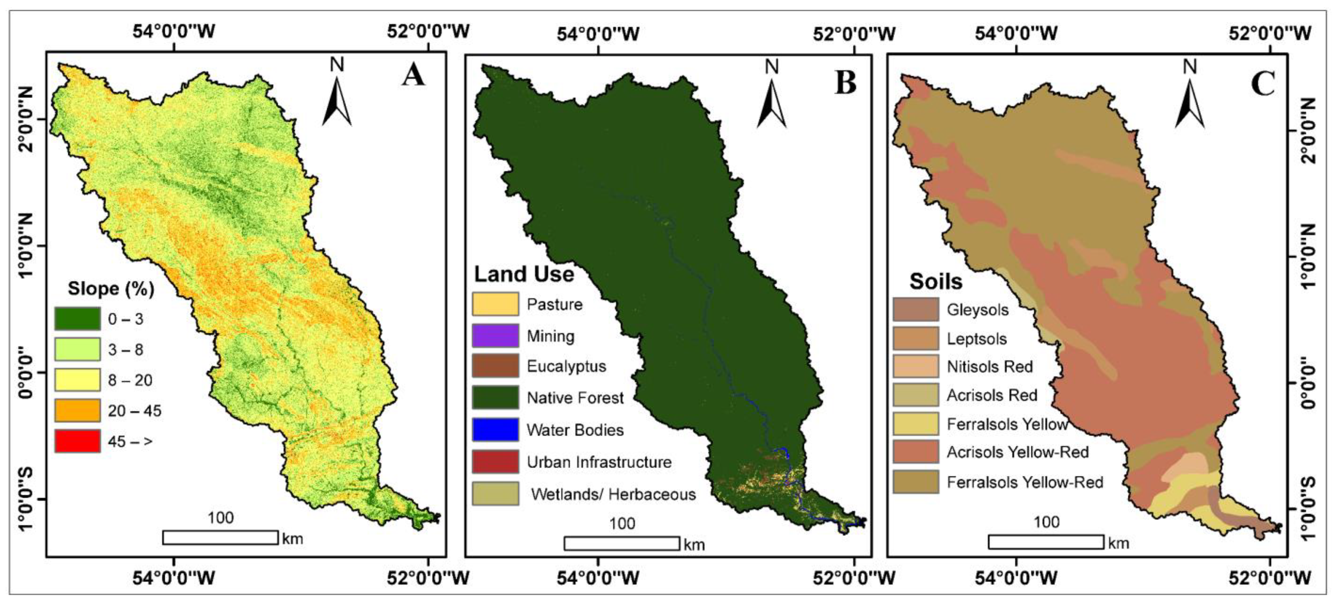
2.1. Study Area

The Jari River Watershed (JRW; Figure 1) covers 57,000 km2 and is located on the Brazilian border, between the Brazilian states Pará and Amapá, and Suriname, and French Guiana, between the latitudes 02°39′02″ N and 01°26′24″ S and the longitudes 51°47′24″ W and 55°07′48″ W. The Jari River has its source at the border with Suriname in a region called “Colinas do Amapá” and has a meandering course with an extension of approximately 950 km. It is a left-bank tributary to the Amazon River. Regarding vegetation cover, dense ombrophilous forests, crossed by alluvial forests, dominate the JRW. Other forest formations occur depending on environmental factors, such as geomorphology and altitude. The vegetation of the JRW is considered preserved in most of the basin [34,35].
Regarding human occupation, human interference and impacts are minimal in the upper and middle JRW, and pristine forests are frequent. In the lower JRW, i.e., the south, the municipalities Laranjal do Jari, Vitória do Jari, and Monte Dourado are the most human-impacted areas with large-scale industrial complexes, such as the Jari Cellulose company and Santo Antônio do Jari Hydroelectric Power Plant [34,36,37].
The prevailing climate in the JRW is humid tropical, according to the Köppen-Geiger classification [38]. The JRW has a warm climate, with a short annual dry period of one to two months (September and October) and an intense rainfall regime during the rest of the year (total average annual precipitation > 1500 mm) (Figure 2). The highest rainfall occurs in the southeast and northeast portions, exceeding 2200 mm per year, while the lowest rainfall occurs in the northwest and southwest portions of the basin (Figure 2). The main climatic systems affecting precipitation and temperature in the region are (i) the Intertropical Convergence Zone (ITCZ), which is considered to be the principal atmospheric system acting over the equatorial region in precipitation generation, and (ii) lines of instability, considered to be Convective Mesoscale Systems (MCSs) responsible for a significant part of the precipitation in the basin by the formation and excess of rainfall at the border region between Amapá and Pará states, mainly during summer [39,40,41].

2.2. Digital Elevation Model (DEM)

To delineate the JRW and its drainage system, we utilized the Digital Elevation Model (DEM) based on the Shuttle Radar Topography Mission (SRTM) [42]. This data comprises locations between 60° North and 56° South, with an original spatial resolution of 90 m refined to 30 m. SRTM data can be downloaded from the United States Geological Survey (USGS) at: https://earthexplorer.usgs.gov/ (accessed on 21 January 2019) [42]. The altimetry of the JRW, derived from SRTM, is shown in Figure 1 (Study area), and the slope is presented in Figure 3A.

2.3. Land Use and Land Cover

We used the MapBiomas annual Land Use Land Cover (LULC) maps collection 6.0 provided at a spatial resolution of 30 m to represent LULC in SWAT for HRU delineation. MapBiomas LULC maps are available for the Brazilian territory since 1985 based on Landsat-derived images. We used one annual LULC map corresponding to the year 2018 to run SWAT. For each land use type, a total of eight physical parameters were obtained from the literature [43,44,45,46,47,48,49] to characterize land use for hydrologic modeling of the study region. Examples of these parameters are Manning’s “n” value for overland flow, the maximum potential leaf area index, the maximum canopy height (m), the maximum root depth (m), the fraction of total potential heat units for the first and second point of leaf area development, and the fraction of the maximum leaf area index for the first and second point of leaf area development [50]. The map used in this project for the year 2018 can be found at: https://mapbiomas.org/ (accessed on 22 June 2020) and downloaded for the Google Earth Engine Platform [51,52]. The spatial distribution of LULC in the study area is shown in Figure 3B.

2.4. Soil

For HRU delineation, SWAT required the representation of soils across the JRW. This information was obtained from the Empresa Brasileira de Pesquisa Agropecuária (EMBRAPA) soil map for 2011, provided at a scale of 1:5,000,000 following the Brazilian Soil Classification System of 2006 [53]. For each soil type, a total of 19 physical parameters were obtained from the literature [54,55,56] to characterize soils for hydrologic modeling of the study region. Examples of these parameters are soil name, soil hydrologic group (A, B, C, or D), the maximum rooting depth of the soil profile (mm), the depth from soil to the bottom of layer (mm), and the saturated hydraulic conductivity (mm/h). More information about these parameters is given in the SWAT documentation [50]. The spatial distribution of the soil types in the study area is shown in Figure 3C.

2.5. Climate Data

Daily climate data are necessary to run SWAT, which includes precipitation, the maximum and minimum temperature (°C), air relative moisture (%), wind speed (m/s), and solar radiation (MJ/m2). Except for precipitation, all other climate input data were obtained from the global climate database Global Weather Data for SWAT (GWDS), which is based on the National Centers for Environmental Prediction (NCEP) for a period of 36 years (1979–2014), denominated Climate Forecast System Reanalysisv3 (CFSR.v3) (available at: https://globalweather.tamu.edu/ (accessed on 23 May 2019)) [57].
The precipitation input to hydrological models is one of the most important. It controls the representation of the flow simulation and the water balance of the watershed. Therefore, accurate precipitation data considering temporal and spatial variability is the key to the simulation process, evaluation of water variability, and forecasting [58,59,60,61,62]. The daily precipitation data for SWAT modeling of the study region was extracted from the Climate Hazards Group Infrared Precipitation with Stations (CHIRPS) dataset [63]. CHIRPS consists of global daily precipitation estimates based on infrared Cold Cloud Duration (CCD) observations, with a spatial resolution of 5 km, covering 50° S–50° N latitudes and all longitudes. This dataset offers daily estimates since 1981 and has been developed jointly by the United States Geological Survey (USGS) and the Climate Hazards Group (CHG). CHIRPS estimates are based on numerous datasets, including ground station data [63]. This dataset was used to represent precipitation in the study area because there were only a few meteorological stations in the JRW. Moreover, CHIRPS was previously assessed in the ARB and accurately represented precipitation patterns in this region [64]. Gridded climatological points were used for the climatic data due to the inexistence of conventional weather stations. Fifty points were established across the basin, providing representative climate data stations for the simulation.

2.6. Flow Data

For the calibration and validation of SWAT simulations, we used monthly streamflow data from the Agência Nacional de Águas (ANA) [65]. We used historical flow data series corresponding to the period from 1981 to 2013 from the São Francisco station (ANA code: 19150000) (Figure 1) [65]. This gauge is the only gauging station in the JRW that offers daily and monthly flow data for the entire simulation period (1981–2013). Throughout the entire historical series analyzed, no significant LULCC was identified in the area influencing this station [52].

2.7. SWAT Model

In the configuration of the SWAT Model, the JRW was initially delineated into sub-basins based on a detailed topographic map of the region (see Section 3.2) and subsequently into multiple hydrological response units (HRUs). These HRUs were formed to represent homogeneous areas with similar characteristics related to soil, LULC, and topography. These combinations in each sub-basin enable the model to simulate land phase physical processes, such as surface runoff, evapotranspiration, and other water balance components. Initially, the model calculates the water balance for each HRU and then aggregates the estimates for each sub-basin [18,66]:
S W t = S W 0 + i = 1 t ( R d a y Q s u r f E a W s e e p Q g w )
where: SWt is the final soil water content (mm H2O); SW0 is the initial soil water content on day i (mm H2O); Rday is the amount of precipitation on day i (mm H2O); Qsurf is the amount of surface runoff on day i; Wseep is the amount of water entering the vadose zone from the soil profile on day i (mm H2O); Qgw is the amount of return flow on day i (mm H2O); Ea is the amount of evapotranspiration on day i and t is the time (days) [16,18].
Subsequently, the model simulates the in-stream or routing phase processes that are associated with the propagation of water, sediment, nutrients, or pesticides through the channels and out of the watershed [18,66].

2.8. Configuration of the Model

To run simulations, we used SWAT version 2012 coupled with the geographic information system ArcGIS version 10.5. In the first step, we outlined the watershed with its drainage network based on the STRM DEM, and 126 sub-basins were obtained. Subsequently, we defined HRUs based on singular combinations of soils, LULC, and slope (Figure 3). The MapBiomas-derived LULC was reclassified based on the SWAT LULC classes. The slope classes were defined as: (i) flat (0–3%); (ii) gently wavy (3–8%); (iii) undulating (8–20%); (iv) heavy wavy (20–45%); and (v) mountainous (>45%) according to classifications defined by EMBRAPA [53]. During this initial step, a reduction factor of 5% was applied. After these procedures, we defined 856 HRUs in the study area.
Subsequently, we inserted the climate data derived from meteorological data in the model. The 50 gridded climatological points across the WJR were based on CHIRPS and Reanalysis data. Historical data was available from 1981 to 2013 (33 years), considering that reanalysis data finished in mid-2014 on the SWAT website. The period from 1981 to 1983 was used as the equilibrium warm-up period for the model to simulate the water balance adequately. These years were excluded from the model results [50,66]. Therefore, we used a simulation period of 30 years, from 1984 to 2013. The method for calculating potential evapotranspiration, utilizing Priestley-Taylor, is based on previous tests of the equations available in the SWAT model.
After finishing the basic configuration of the SWAT model, we set other supplementary configurations, aiming at improving the simulation of the study area, following Arroio Junior [49]. First, the parameters related to LULC (Topic 2.2), which SWAT uses to estimate plant growth under ideal conditions, were modified. These parameters were based on the development of the leaf area and the interception and conversion of sunlight into biomass. More information about these parameters is given in the SWAT theoretical documentation [18].

2.9. Calibration and Validation

In this step, the flow simulation derived from SWAT was calibrated and validated [67]. These procedures were conducted with the Calibration and Uncertainty Procedures—SWAT CUP version 5.2.1.1 software [68]. This independent software calibrates, validates, and evaluates the uncertainties of SWAT-derived simulations. In this program, it is possible to utilize approaches such as the Generalized Likelihood Uncertainty Estimation (Glue), Particle Swarm Optimization (PSO), Parameter Solution (ParaSol), Sequential Uncertainty Fitting version 2 (SUFI-2), and Markov Chain Monte Carlo (MCMC) to evaluate the simulations derived from SWAT [67,68]. In this research, we utilized SUFI-2 since this approach is more efficient for calibrating large basins such as the JRW [67].
In SUFI-2, the input parameter uncertainty is expressed in the form of uniform distributions, while the uncertainty of the outputs is represented and evaluated by the probability distribution uncertainty of 95 percent (95%PPU) [69]. The 95PPU is calculated from the 2.5% and 97.5% levels based on cumulative distributions of the output variables obtained from Latin Hypercube Sampling (LHS) [69,70]. The LHS is the sampling method used in SUFI-2 to obtain new parameter ranges for the calibration iterations. For uncertainty evaluations, two statistical metrics were calculated; the p-factor and the r-factor. The p-factor indicates the percentage of the measured data (plus their error) that can be reproduced by the model predictions. The r-factor indicates the thickness of the envelope of 95PPU. The combination of these two factors indicates the power of the calibration and the evaluation of uncertainty associated with the model. As a recommendation, the p-factor for large-scale modeling should be greater than 0.75 and the r-factor should be lower than 1.5 for these metrics [67,68,69].
To calibrate the model, we first performed a sensitivity analysis to identify the parameters that strongly affect the performance of the model [71]. We performed Global Sensitivity Analysis, which determines changes in the multiple regression from the input variables where the sensitivities are changes in the average of the objective function derived from changes in each parameter. This method provides the relative sensitivities based on linear approaches from the t-stat and p-value, where the higher the absolute value of the t-stat (ratio of the coefficient of a parameter to its standard error) and the lower the p-value (the null hypothesis is that the coefficient is equal to zero, i.e., no effect), the more sensitive the parameter [68]. The selection of the parameters utilized for this step and the following calibration and validation steps were based on the model’s initial outputs and the calibration protocols for large-scale distributed models suggested by Abbaspour [67] and used in previous studies in Amazonian watersheds, such as [72,73]. In addition, this step determined the objective function, which utilized the function bR2 [74], described in Equation (2).
= { | b | R 2     i f   | b | 1     | b | 1 R 2   i f   | b | > 1
where R2 is the coefficient of determination, b is the regression coefficient between measured and simulated data. For the determination of bR2, the coefficient of determination R2 is multiplied by the regression coefficient [74]. More information can be found on [68,74].
The inclusion of b also ensures that the predictions of under- and overestimates of the flow are reflected. The major advantage of this criterion is its range from 0 to 1, which can vary considerably in other metrics, for example, to −∞ in NS [67,74,75].
Subsequently, the model was calibrated for the 1984–2003 period by executing multiple iterations, with 1000 runs in each iteration until the simulated results were statistically satisfactory, according to the metrics proposed by Moriasi [76]. Satisfactory results were achieved in terms of the p-factor (>0.75) and r-factor (<1.5) or when there was no significant increase in the results obtained by the objective function, as suggested by Abbaspour [67]. Then, the model was considered calibrated [67]. After calibration, started the validation process, in which the model performance was tested against an independent data series not used during the calibration step. For the validation procedure, we utilized hydrologic data from 2004–2013 [67].
For evaluating the resulting calibration and validation, we utilized the statistical metrics (Table 1) for a monthly time step of stream flow, as recommended by Moriasi [76].
The percent bias (PBIAS) represents the simulated data tendency data and its deviation from observed values. In this metric, low values indicate a satisfactory model simulation [77]. The PBIAS is calculated according to Equation (3).
P B I A S = i = 1 n ( q i o b s q i s i m ) i = 1 n ( q i o b s ) × 100
where q is a model variable (e.g., stream flow, sediments), obs is the ground truth measurement, and sim is the simulated value [77].
The Nash-Sutcliffe coefficient (NS) is a normalized metric representing the change in relative magnitude data compared to measured variance data and ranges between −∞ and 1 [78]. The NS is calculated according to Equation (4).
N S = 1 i ( Q m Q s ) i 2 i ( Q m , i Q ¯ m ) 2
The standard deviation ratio (RSR) is a metric that incorporates the benefits of the root-mean-square error index (RMSE) with a normalization factor, where the resulting statistics and the described values can be applied to various components. This metric ranges from an excellent value of 0 to a great value, where 0 indicates no residual variation and, consequently, a perfect simulation of the model [76]. The RSR is calculated according to Equation (5).
R S R = i = 1 n ( Q m Q s ) i 2 i = 1 n ( Q m , i Q ¯ m ) 2
In addition, we utilized the coefficient of determination (R2), a statistical metric that describes the degree of collinearity between simulated and measured data [76,79,80]. The R2 is calculated according to Equation (6).
R 2 = [ i ( Q m , i Q ¯ m ) ( Q s , i Q ¯ s ) ] 2 i ( Q m , i Q ¯ m ) 2 i ( Q s , i Q ¯ s ) 2

3. Results

This section describes the results obtained from running SWAT in the study area. Initially, we describe the sensitivity analyses, followed by the model calibration and validation results. Then, we show the results regarding the statistical metrics for assessing the model runs and the spatial distribution of the model outputs in the JRW.

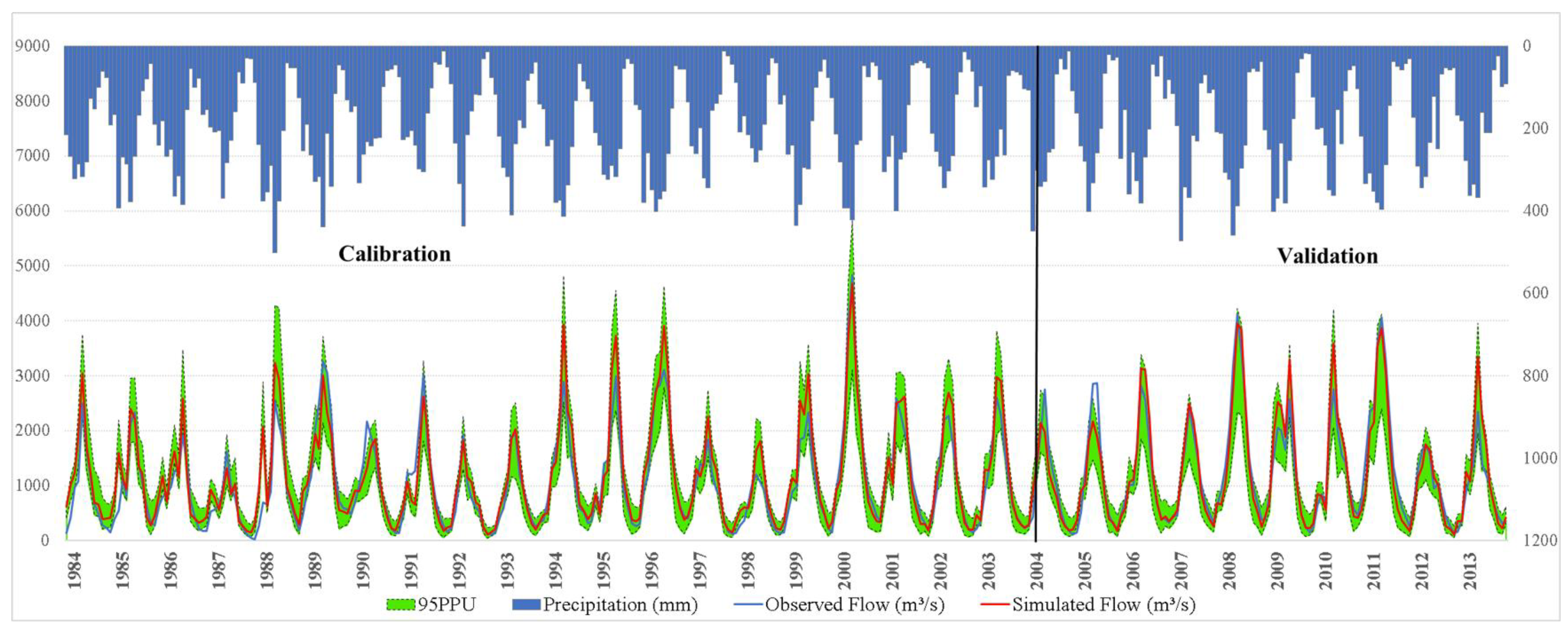
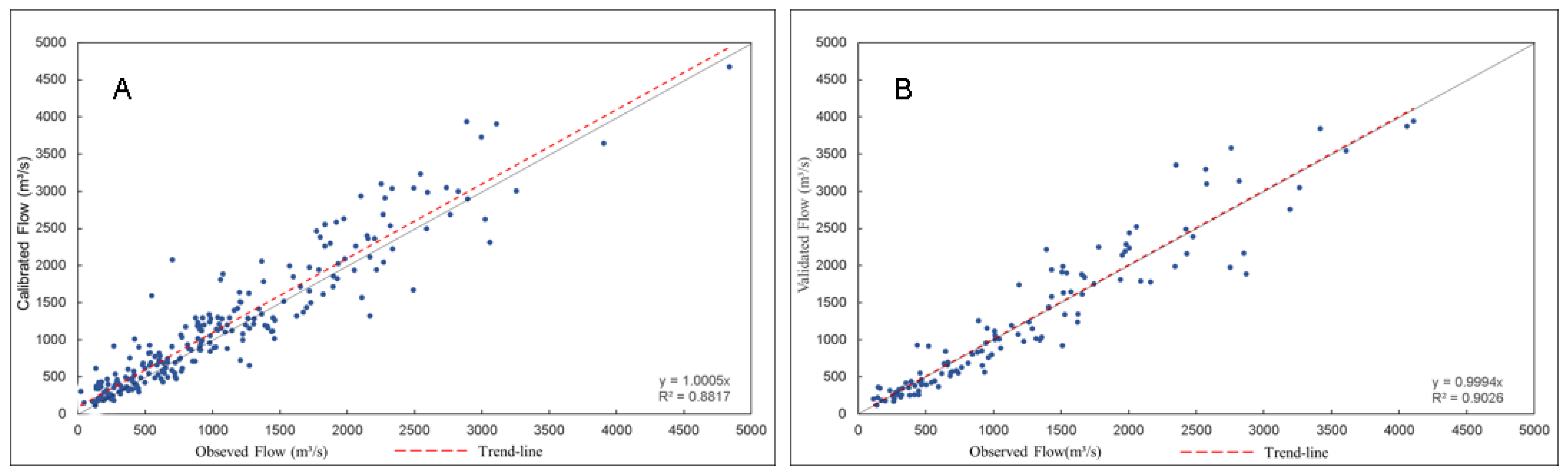
3.1. Sensitivity Analyses, Calibration, and Validation

For the execution of the sensitivity analyses, we selected 18 parameters based on the initial model results, as determined by the intervals of variation for each parameter (minimum and maximum) with the same range as that used in calibration (Table 2). The parameter change methods used were the substitution method, in which the default value of the parameter was replaced by a given value, and the multiplication method, in which the parameter value is multiplied by 1+ a given value [68]. In the sensitivity analysis step, the hydrological years 1984–2003 were used, and this period was utilized later in the calibration. The results of this analysis are summarized in Table 3. The most sensitive parameter was v_RCHRG_DP.gw, followed by r_CN2.mgt, v_GW_DELAY.gw, r_SOL_AWC().sol, and r_SOL_K().sol. The other parameters, v_ALPHA_BF, v_GW_REVAP, v_CANMX.hru_FRSE, v_CH_N2.rte, v_CH_K2.rte, v_ESCO.hru, and v_REVAPMN.gw, showed a decrease in sensitivity. The parameters v_EPCO.hru and r_SOL_ALB().sol had the lowest sensitivity. Consequently, they had little influence on the model outputs.
After the sensitivity analysis, the model was calibrated. We used the same period (1984–2003, 20 hydrological years) during the calibration. Additionally, we used the 1981–1983 period for the model warm-up using the parameters of the previous step. We realized two repetitions with 1000 simulations each. The model was considered calibrated due to the good statistical results based on the statistical metrics described in Moriasi and Abbaspour [67,76] (Table 1), where no further improvements on the objective function results were found. Following calibration, we performed the validation based on different and independent data series of 10 hydrological years (2004–2013).
The model obtained very good results during the calibration and validation process according to the statistical metrics proposed by Moriasi [76] (Table 2). A good agreement with NS (0.85 and 0.89), RSR (0.39 and 0.33), and PBIAS (−9.5 and −0.6) was found for the calibration and validation steps, respectively. Additionally, the model achieved R2 values of 0.88 and 0.90 for the calibration and validation, respectively. Regarding bR2, the metric utilized to evaluate the objective function, values obtained were similar to R2. The SWAT model generally performed well, even when running the model based on meteorological data. The p-factor and r-factor metrics were 0.84 and 0.93, and 0.84 and 0.78 for the calibration and validation, respectively. These results showed the robustness of the SWAT model.
The hydrograph in Figure 4 shows the flow simulation after calibration and validation with 95PPU uncertainty bands. The model expressed the flow more satisfactorily after the calibration procedure due to peak flow reduction and a better baseflow adjustment. In the validation period 2004–2013, these improvements outperformed the calibration results, and the peak flow and baseflow had a good adjustment with the observed flow.
The dispersion diagram (Figure 5) reinforced the results described above, and strong correlations between the simulated flow and observed flow were found (significant at 0.05 level by student t-test).

3.2. Water Balance Components

After the calibration of the model, we obtained the monthly water balance of the JRW for 1984–2013. Additionally, we calculated annual estimates based on the monthly estimates to interpret the results better. For precipitation, we obtained a monthly average of 184.38 mm and an annual average of 2212.56 mm. For evapotranspiration, average monthly and annual values were 109.85 mm and 1318.25 mm, respectively. For percolation, we observed average values of 36.08 mm (monthly) and 432.96 mm (annual). The average baseflow was 16.72 mm (monthly) and 200.7 mm (annual). Finally, the water balance component with the lowest observed values, with average values of 4.24 mm (monthly) and 50.89 mm (annual), was the surface runoff.

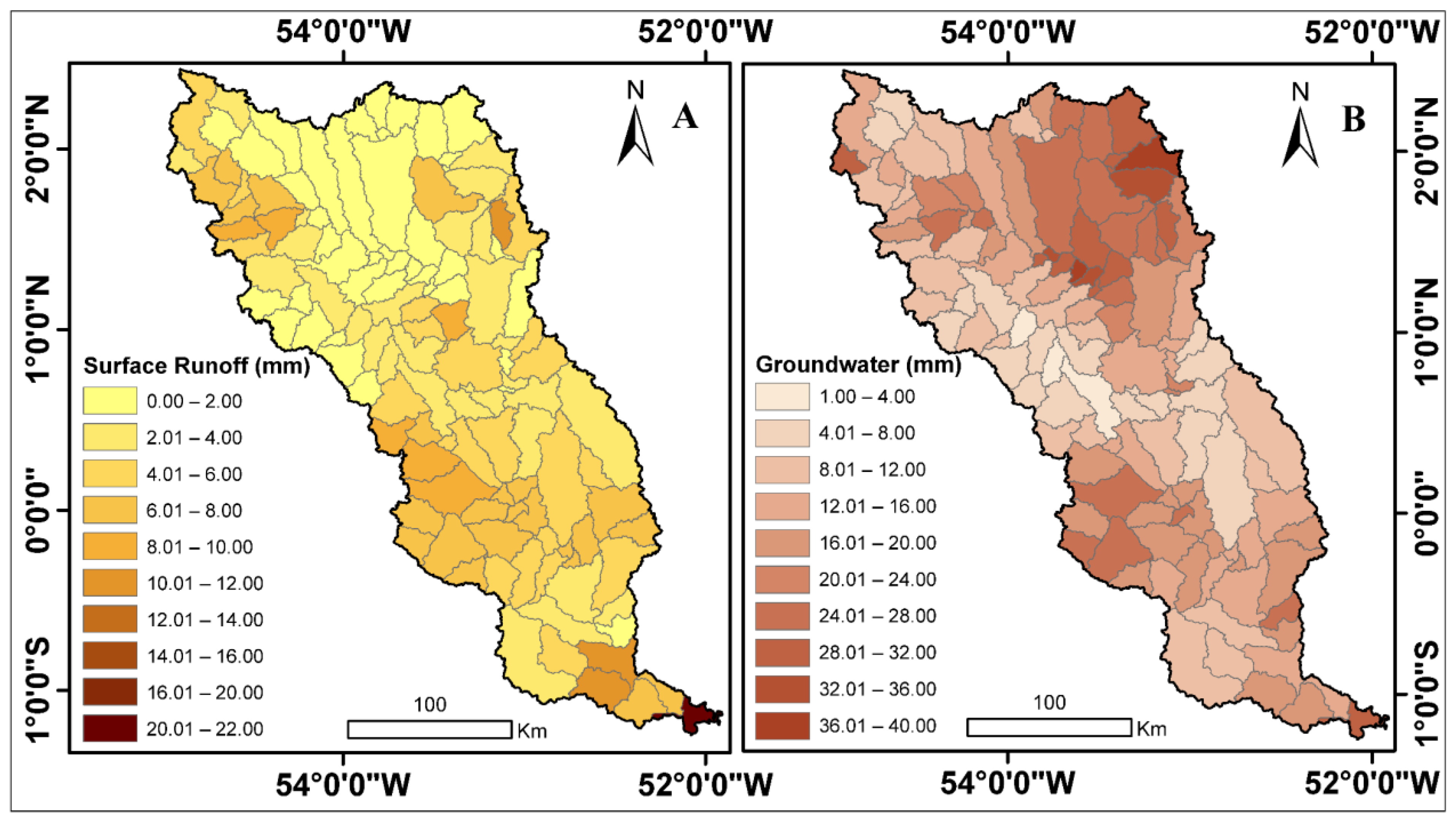
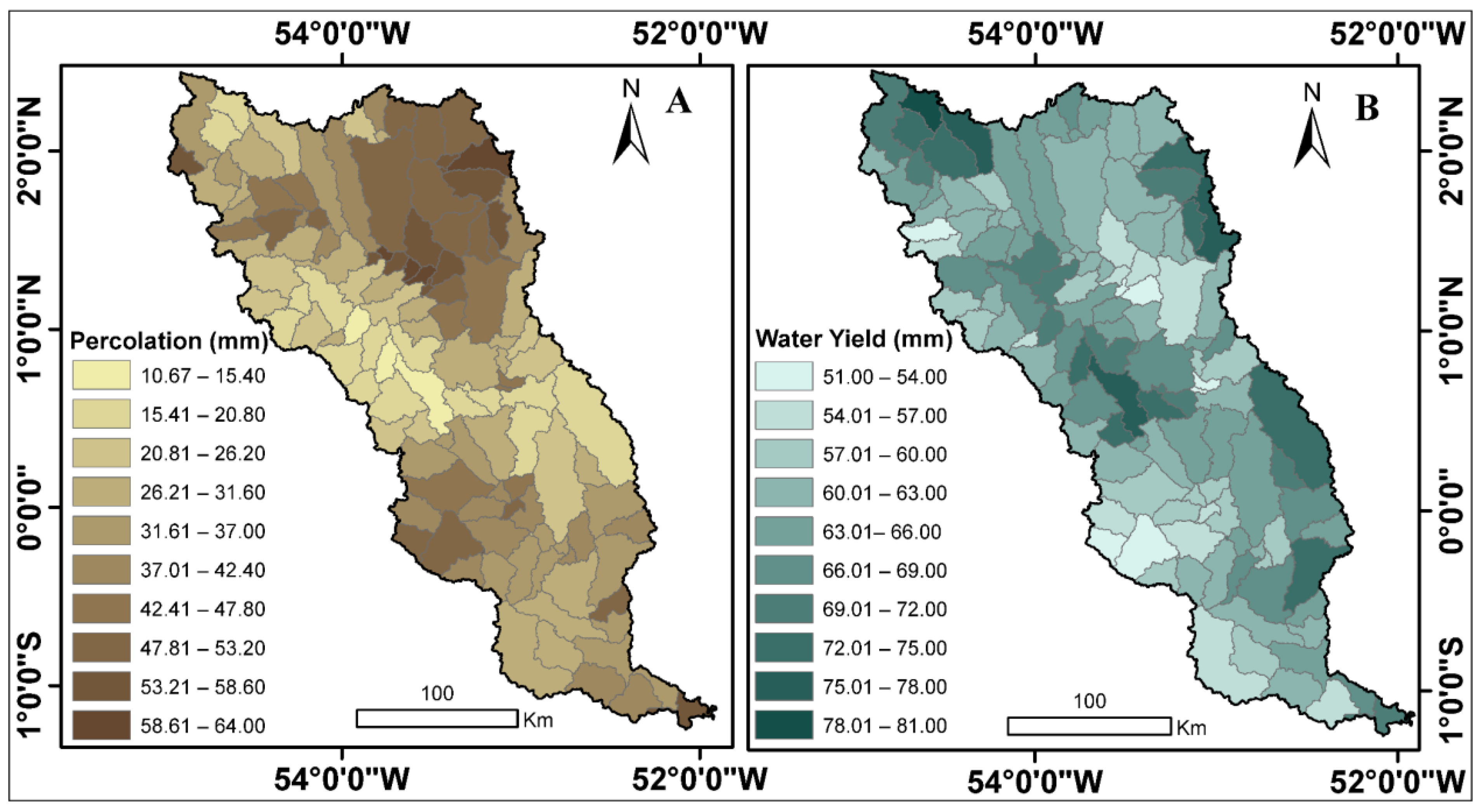
3.3. Spatial Distribution of Water Balance Components

The spatial distribution of the water balance components is shown in Figure 6, Figure 7 and Figure 8. Figure 6A shows the spatial distribution of the simulated precipitation for the sub-basins of the JRW estimated using CHIRPS from 1984 to 2013. The monthly average values were higher than 160 mm in all sub-basins, reaching a maximum average of 200 mm per month. These higher values were concentrated in the north, northeast, southeast, and south of the JRW. On the other hand, the western part of the JRW showed the lowest values. Figure 6B shows the spatial distribution of the results for evapotranspiration in the JRW. This water balance component had monthly average values higher than 60 mm in all sub-basins, reaching a maximum average of 121 mm per month. The highest values were found in the study area’s northern, northeastern, and southern regions. The central and western regions had the lowest values for this component.
Figure 7A shows the spatial distribution of the surface runoff simulation results in the JRW. This component showed a low average when compared with other water balance components. The monthly average values ranged from less than 1 to 22 mm in the southern portion of the basin. Figure 7B shows the spatial distribution of the groundwater simulation results. This component had a monthly average value higher than 1 mm in all sub-basins, reaching the maximum average of 40 mm per month. The highest values were concentrated in the northern and southern-central regions of the JRW.
Figure 8A shows the spatial distribution of the simulated percolation in the JRW. The monthly average percolation ranged from 10 to 64 mm, with higher values in the northern, northeastern, south-central, and southern regions of the JRW. Other regions, such as the northwestern and central regions, showed lower average values. Finally, Figure 8B shows the spatial distribution of the simulated water yield in the study area. This component had monthly average values higher than 51 mm in all basins, reaching a maximum average of 81 mm in the northern and central regions. The southern and southwestern regions had the lowest values for this component.

4. Discussion

The present study assessed the efficiency of the SWAT model for simulating water flow and balance components in a poorly monitored Amazonian basin based on orbital data. The results showed that the SWAT model efficiently executed these simulations. Regarding sensitivity analysis, the most prominent parameters were RCHRG_DP, CN2, and GW_DELAY. These parameters are strongly related to the controls of groundwater processes and surface runoff. Singh [81] used SWAT to simulate the water flow and hydrologic balance components of the Ib River watershed (India) and obtained similar results. RCHRG_DP and CN2 were the most sensitive parameters. However, according to the authors, the CN2 parameter indicated rapid LULCC, while the RCHRG_DP indicated rapid water movement to the deep aquifer.
Schmalz [82] used the same approach in catchments located in Germany. In this study, the most sensitive parameters were groundwater-related, including RCHRG_DP. According to the authors, this indicated that water flow in the studied lowland region was heavily influenced by infiltration. Considering the previous results and that the JRW is composed of low slopes and highly preserved, the infiltration process should predominate over runoff, which can influence the sensitivity of the parameters.
Regarding the calibration and validation steps, the results showed a good agreement between the simulated and the observed flow (Figure 4), as corroborated by the statistical results obtained (Table 2) and according to the metrics proposed by Abbaspour [67] for the calibration of large basins as well as the statistical metrics proposed by Moriasi [76]. Similar results were reported in Lopes [83] using SWAT to model the availability of water, hydrological regime, and the impacts of LULC in the Teles Pires River, in the Southern Brazilian Amazon. The results of this study showed that SWAT performed well, with good results regarding statistical terms. SWAT was able to generate flow data efficiently, even in a basin with scarce data. Similarly, Serrão [84] used SWAT to assess the impacts of LULCC on hydrological processes in the Itacaúnas River in the eastern Amazon region of Brazil and demonstrated agreement between simulated and observed flow regarding seasonality.
It is evident that the methodological choices made, i.e., the choice of data, the selection of calibration parameters, and the choice of the objective function have considerable influence on the results. According to the comparison with the only gauging station in the JRW, the model was considered very efficient in simulating the water flow in the study area. Due to the lack of observational data in the JRW, as pointed out by Bressiani [85], the approach of this work was successful. The challenges discussed so far stress the importance of hydrological modeling for the ARB and similar watersheds.
In terms of water balance, similar results were obtained in other basins in the Amazon, e.g., by Abe [71], when using SWAT to model the Upper Creposi River basin located in the ARB. The authors obtained a mean annual evapotranspiration of 1300 mm, surface runoff was less than 50 mm, and the shallow aquifer had values below 1200 mm annually in 1973. Other components of the water balance were not evaluated in this study. Another example is the work of Santos [73], using SWAT to model the Iriri River watershed, also in the ARB. This study reported that about 50% of the rainfall over the watershed returned to the atmosphere as evapotranspiration. However, the surface runoff showed values below 10% of the rainfall recorded in the basin.
Comparing the results of the JRW with those of the Upper Creposi River basin [72] and the Iriri River basin [73], there was good agreement between evapotranspiration results, ranging from 50 to 60% of the estimated precipitation of the three basins. However, lower values were found for other hydrologic water balance components, such as the shallow aquifer and surface runoff. This difference may be related to specific and intrinsic factors related to the physical characteristics of the basins. Although all three watersheds are in the ARB, they have different types of soils and LULC that play an important role in the hydrological dynamics of these watersheds.

5. Conclusions

This study aimed to analyze hydrological processes in a poorly monitored Amazon basin with a high degree of preservation based on orbital data such as reanalysis data and CHIRPS. This research showed that SWAT was efficient in the simulation of water balance and flow, representing their spatiotemporal dynamics adequately. We demonstrated the suitability of SWAT for the Amazon region and the good accuracy of this model in simulations with only one calibration point. Furthermore, calibration and validation results corroborated the efficiency of SWAT applied to the ARB. Statistically, the results of this research showed a good performance for the calibration and validation, obtaining results considered “very good” according to the metrics used. Consequently, it represented the water balance in an equatorial environment.
The importance of this study is in the evaluation of the efficiency of SWAT in conjunction with input data from unconventional sources, i.e., data not measured in the field (CHIRPS and Reanalysis) for other Amazonian basins that lack field data. Our results enable the use of SWAT in other hydrological studies, including those related to the water balance, sediment transport, water quality, and evaluations of the impacts of climate change and deforestation. Considering that SWAT is a powerful modeling tool and allows numerous environmental applications, we highlight its great importance for studies in the Amazon, which acts as a climate regulator and lacks studies that use modeling for such assessments.
Additionally, considering precipitation as the main water input to the basin and responsible for water balance controls, other data sources, such as other reanalysis products, should be evaluated for the execution of future simulations. Such sources could represent the basin’s climate more precisely, considering the generally good model performance for tropical basins based on orbital data.

Author Contributions

Conceptualization, P.R.R. and G.P.; methodology, P.R.R., G.P., B.G. and M.F.; formal analysis, P.R.R. and G.P.; writing—original draft preparation, P.R.R., G.P., G.D.Z. and P.R.S.; writing—review and editing, P.R.R., G.P., P.R.S., F.d.S.C., B.G., I.G.B. and G.M.; visualization, P.R.R. and G.P.; supervision, G.P. and B.G. All authors have read and agreed to the published version of the manuscript.

Funding

P.R.R. thanks the Coordenação de Aperfeiçoamento de Pessoal de Nível Superior (CAPES, grant 88882.461730/2019-01), G.M. thanks the São Paulo Research Foundation (FAPESP, grant 2019/25701-8), G.P. thanks the National Council for Scientific and Technological Development (CNPq, grants 307004/2020-1 and 441934/2018-8).

Data Availability Statement

All data and code used in the current study are available from the corresponding author on reasonable request.

Acknowledgments

The authors are grateful to the Federal University of São João del-Rei (UFSJ) and to the Programa de Pós-Graduação em Geografia (PPGeog) of UFSJ for supporting the development of this research. We are also grateful to the Watershed Science and Modelling Laboratory (WSML) at the Department of Earth and Atmospheric Sciences for supporting the development of this research.

Conflicts of Interest

The authors declare no conflict of interest.

References

  1. Ritter, C.D.; Zizka, A.; Barnes, C.; Nilsson, R.H.; Roger, F.; Antonelli, A. Locality or Habitat? Exploring Predictors of Biodiversity in Amazonia. Ecography 2019, 42, 321–333. [Google Scholar] [CrossRef] [Green Version]
  2. Paredes-Trejo, F.; Barbosa, H.; Giovannettone, J.; Kumar, T.V.L.; Kumar Thakur, M.; de Oliveira Buriti, C. Drought Variability and Land Degradation in the Amazon River Basin. Front. Earth Sci. 2022, 10, 1–16. [Google Scholar] [CrossRef]
  3. Fassoni-Andrade, A.C.; Fleischmann, A.S.; Papa, F.; de Paiva, R.C.D.; Wongchuig, S.; Melack, J.M.; Moreira, A.A.; Paris, A.; Ruhoff, A.; Barbosa, C.; et al. Amazon Hydrology From Space: Scientific Advances and Future Challenges. Rev. Geophys. 2021, 59, e2020RG000728. [Google Scholar] [CrossRef]
  4. Chaudhari, S.; Pokhrel, Y. Alteration of River Flow and Flood Dynamics by Existing and Planned Hydropower Dams in the Amazon River Basin. Water Resour. Res. 2022, 58, e2021WR030555. [Google Scholar] [CrossRef]
  5. Van Der Ent, R.J.; Savenije, H.H.G. Length and Time Scales of Atmospheric Moisture Recycling. Atmos. Chem. Phys. 2011, 11, 1853–1863. [Google Scholar] [CrossRef] [Green Version]
  6. Keys, P.W.; Wang-Erlandsson, L.; Gordon, L.J. Revealing Invisible Water: Moisture Recycling as an Ecosystem Service. PLoS ONE 2016, 11, e0151993. [Google Scholar] [CrossRef] [PubMed]
  7. O’Connor, J.C.; Santos, M.J.; Dekker, S.C.; Rebel, K.T.; Tuinenburg, O.A. Atmospheric Moisture Contribution to the Growing Season in the Amazon Arc of Deforestation. Environ. Res. Lett. 2021, 16, 084026. [Google Scholar] [CrossRef]
  8. Silva, C.V.J.; Aragão, L.E.O.C.; Barlow, J.; Espirito-Santo, F.; Young, P.J.; Anderson, L.O.; Berenguer, E.; Brasil, I.; Brown, I.F.; Castro, B.; et al. Drought-Induced Amazonian Wildfires Instigate a Decadal-Scale Disruption of Forest Carbon Dynamics. Philos. Trans. R. Soc. B Biol. Sci. 2018, 373, 20180043. [Google Scholar] [CrossRef] [Green Version]
  9. Libonati, R.; Pereira, J.M.C.; Da Camara, C.C.; Peres, L.F.; Oom, D.; Rodrigues, J.A.; Santos, F.L.M.; Trigo, R.M.; Gouveia, C.M.P.; Machado-Silva, F.; et al. Twenty-First Century Droughts Have Not Increasingly Exacerbated Fire Season Severity in the Brazilian Amazon. Sci. Rep. 2021, 11, 4400. [Google Scholar] [CrossRef]
  10. Staal, A.; Flores, B.M.; Aguiar, A.P.D.; Bosmans, J.H.C.; Fetzer, I.; Tuinenburg, O.A. Feedback between Drought and Deforestation in the Amazon. Environ. Res. Lett. 2020, 15, 044024. [Google Scholar] [CrossRef]
  11. Zemp, D.C.; Schleussner, C.F.; Barbosa, H.M.J.; Hirota, M.; Montade, V.; Sampaio, G.; Staal, A.; Wang-Erlandsson, L.; Rammig, A. Self-Amplified Amazon Forest Loss Due to Vegetation-Atmosphere Feedbacks. Nat. Commun. 2017, 8, 14681. [Google Scholar] [CrossRef] [PubMed] [Green Version]
  12. Villén-Pérez, S.; Moutinho, P.; Nóbrega, C.C.; De Marco, P. Brazilian Amazon Gold: Indigenous Land Rights under Risk. Elem. Sci. Anthr. 2020, 8, 31. [Google Scholar] [CrossRef]
  13. Mataveli, G.; Chaves, M.; Guerrero, J.; Escobar-Silva, E.V.; Conceição, K.; de Oliveira, G. Mining Is a Growing Threat within Indigenous Lands of the Brazilian Amazon. Remote Sens. 2022, 14, 4092. [Google Scholar] [CrossRef]
  14. Furtado Louzada, A.; Ravena, N. Dam Safety and Risk Governance for Hydroelectric Power Plants in the Amazon. J. Risk Res. 2019, 22, 1571–1585. [Google Scholar] [CrossRef]
  15. Freitas, C.E.; de Almeida Mereles, M.; Pereira, D.V.; Siqueira-Souza, F.; Hurd, L.; Kahn, J.; Morais, G.; Sousa, R.G.C. Death by a Thousand Cuts: Small Local Dams Can Produce Large Regional Impacts in the Brazilian Legal Amazon. Environ. Sci. Policy 2022, 136, 447–452. [Google Scholar] [CrossRef]
  16. Arnold, J.G.; Srinivasan, R.; Muttiah, R.S.; Williams, J.R. Large Area Hydrologic Modeling and Assessment Part I: Model Development. J. Am. Water Resour. Assoc. 1998, 34, 73–89. [Google Scholar] [CrossRef]
  17. Yamini Priya, R.; Manjula, R. A Review for Comparing SWAT and SWAT Coupled Models and Its Applications. Mater. Today Proc. 2020, 45, 7190–7194. [Google Scholar] [CrossRef]
  18. Neitsch, S.L.; Arnold, J.; Kiniry, J.; Williams, J. Soil & Water Assessment Tool Theoretical Documentation Version 2009. Texas Water Resour. Inst. 2011, 543, 591–600. [Google Scholar] [CrossRef]
  19. Belvederesi, C.; Zaghloul, M.S.; Achari, G.; Gupta, A.; Hassan, Q.K. Modelling River Flow in Cold and Ungauged Regions: A Review of the Purposes, Methods, and Challenges. Environ. Rev. 2022, 30, 159–173. [Google Scholar] [CrossRef]
  20. Khan, S.R.; Khan, S.R. Assessing Poverty-Deforestation Links: Evidence from Swat, Pakistan. Ecol. Econ. 2009, 68, 2607–2618. [Google Scholar] [CrossRef]
  21. Lucas-Borja, M.E.; Carrà, B.G.; Nunes, J.P.; Bernard-Jannin, L.; Zema, D.A.; Zimbone, S.M. Impacts of Land-Use and Climate Changes on Surface Runoff in a Tropical Forest Watershed (Brazil). Hydrol. Sci. J. 2020, 65, 159–173. [Google Scholar] [CrossRef]
  22. Nazari-Sharabian, M.; Taheriyoun, M.; Ahmad, S.; Karakouzian, M.; Ahmadi, A. Water Quality Modeling of Mahabad Dam Watershed-Reservoir System under Climate Change Conditions, Using SWAT and System Dynamics. Water 2019, 11, 394. [Google Scholar] [CrossRef] [Green Version]
  23. DHI MIKE SHE. User Manual. Volume 2: Reference Guide; MIKE SHE: Hørsholm, Denmark, 2017; Volume 2, pp. 1–372. [Google Scholar]
  24. USACE. Hydrologic Modeling System HEC-HMS User’s Manual CPD-74A; USACE: Washington, DC, USA, 2016; 598p. [Google Scholar]
  25. Lindström, G.; Pers, C.; Rosberg, J.; Strömqvist, J.; Arheimer, B. Development and Testing of the HYPE (Hydrological Predictions for the Environment) Water Quality Model for Different Spatial Scales. Hydrol. Res. 2010, 41, 295–319. [Google Scholar] [CrossRef]
  26. Dhami, B.S.; Pandey, A. Comparative Review of Recently Developed Hydrologic Models. J. Indian Water Resour. Soc. 2013, 33, 34–41. [Google Scholar]
  27. Tan, M.L.; Gassman, P.W.; Yang, X.; Haywood, J. A Review of SWAT Applications, Performance and Future Needs for Simulation of Hydro-Climatic Extremes. Adv. Water Resour. 2020, 143, 103662. [Google Scholar] [CrossRef]
  28. Akoko, G.; Le, T.H.; Gomi, T.; Kato, T. A Review of Swat Model Application in Africa. Water 2021, 13, 1313. [Google Scholar] [CrossRef]
  29. Gassman, P.W.; Reyes, M.R.; Green, C.H.; Arnold, J.G. The Soil and Water Assessment Tool: Historical Development, Applications, and Future Research Directions. Trans. ASABE Am. Soc. Agric. Biol. Eng. 2007, 50, 1211–1250. [Google Scholar] [CrossRef] [Green Version]
  30. Arnold, J.G.; Fohrer, N. SWAT2000: Current Capabilities and Research Opportunities in Applied Watershed Modelling. Hydrol. Process. 2005, 19, 563–572. [Google Scholar] [CrossRef]
  31. Gassman, P.W.; Sadeghi, A.M.; Srinivasan, R. Applications of the SWAT Model Special Section: Overview and Insights. J. Environ. Qual. 2014, 43, 1–8. [Google Scholar] [CrossRef]
  32. Tuo, Y.; Duan, Z.; Disse, M.; Chiogna, G. Evaluation of Precipitation Input for SWAT Modeling in Alpine Catchment: A Case Study in the Adige River Basin (Italy). Sci. Total Environ. 2016, 573, 66–82. [Google Scholar] [CrossRef] [Green Version]
  33. Zhang, G.; Su, X.; Ayantobo, O.O.; Feng, K.; Guo, J. Remote-Sensing Precipitation and Temperature Evaluation Using Soil and Water Assessment Tool with Multiobjective Calibration in the Shiyang River Basin, Northwest China. J. Hydrol. 2020, 590, 125416. [Google Scholar] [CrossRef]
  34. EPE, Empresa de Pesquisa Energética. Bacia Hidrográfica Do Rio Jari/PA-AP Estudos de Inventário Hidrelétrico, AAI—Avaliação Ambiental Integrada Volume 1/2; EP518.RE.JR204 JAR-A-62-000.001-RE-R0; Empresa de Pesquisa Energética: Rio de Janeiro, Brazil, 2011; p. 320. [Google Scholar]
  35. Silveira, J.d.S.d. Aspectos Hidroclimatológicos Da Bacia Do Rio Jari No Periodo de 1968 a 2012. Bachelor’s Thesis, Universidade Federal do Amapá, Macapá, Brazil, 2014; pp. 1–60. Available online: http://repositorio.unifap.br/handle/123456789/502 (accessed on 23 May 2019).
  36. EDP; UHE. Santo Antônio Do Jari. Available online: https://brasil.edp.com/pt-br/uhe-jari (accessed on 4 November 2019).
  37. Oliveira, A.M.; da Cunha, A.C. Indicadores de Vulnerabilidade e Risco Como Subsídios à Prevenção de Impactos à Sociobiodiversidade Na Bacia Do Rio Jari (AP-PA)/Brasil. In Conhecimento e Manejo Sustentável da Biodiversidade Amapaense; Bastos, A.M., Junior, J.P.M., Silva, R.B.L.e., Eds.; Editora Edgard Blücher Ltda.: São Paulo, Brazil, 2017; pp. 161–182. ISBN 978-85-8039-219-7. [Google Scholar]
  38. Alvares, C.A.; Stape, J.L.; Sentelhas, P.C.; De Moraes Gonçalves, J.L.; Sparovek, G. Köppen’s Climate Classification Map for Brazil. Meteorol. Z. 2013, 22, 711–728. [Google Scholar] [CrossRef] [PubMed]
  39. Kodama, Y. Large-Scale Common Features of Subtropical Precipitation Zones (the Baiu Frontal Zone, the SPCZ, and the SACZ) Part I: Characteristics of Subtropical Frontal Zones. J. Meteorol. Soc. Jpn. 1992, 70, 813–836. [Google Scholar] [CrossRef] [Green Version]
  40. Kidd, C.; Huffman, G. Global Precipitation Measurement. Meteorol. Appl. 2011, 18, 334–353. [Google Scholar] [CrossRef]
  41. Ferraro, R.R.; Weng, F.; Grody, N.C.; Zhao, L. Precipitation Characteristics over Land from the NOAA-15 AMSU Sensor. Geophys. Res. Lett. 2000, 27, 2669–2672. [Google Scholar] [CrossRef]
  42. Farr, T.G.; Rosen, P.A.; Caro, E.; Crippen, R.; Duren, R.; Hensley, S.; Kobrick, M.; Paller, M.; Rodriguez, E.; Roth, L.; et al. The Shuttle Radar Topography Mission. Rev. Geophys. 2007, 45, 1–33. [Google Scholar] [CrossRef] [Green Version]
  43. McCuen, R.H. Hydrologig Analysis and Design, 2nd ed.; Pearson Education: Upper Saddle River, NJ, USA, 1998; ISBN 0-13-134958-9. [Google Scholar]
  44. de Almeida, A.C.; Soares, J.V. Comparação Entre Uso de Água Em Plantações de Eucalyptus Grandis e Floresta Ombrófila Densa (Mata Atlântica) Na Costa Leste Do Brasil. Rev. Árvore 2003, 27, 159–170. [Google Scholar] [CrossRef] [Green Version]
  45. Roberts, J.M.; Cabral, O.M.R.; da Costa, J.P.; McWilliam, A.L.C.; Sá, T. An Overview of the Leaf Area Index and Physiological Measurements during ABRACOS. In Amazonian Deforestation and Climate; Gash, J.H.C., Nobre, C.A., Roberts, J.M., Victoria, R.L., Eds.; Wiley and Sons: New York, NY, USA, 1996; pp. 287–305. [Google Scholar]
  46. Samanta, A.; Knyazikhin, Y.; Xu, L.; Dickinson, R.E.; Fu, R.; Costa, M.H.; Saatchi, S.S.; Nemani, R.R.; Myneni, R.B. Seasonal Changes in Leaf Area of Amazon Forests from Leaf Flushing and Abscission. J. Geophys. Res. Biogeosci. 2012, 117, 1–13. [Google Scholar] [CrossRef] [Green Version]
  47. Muller, M.M.L.; Guimarães, M.d.F.; Desjardins, T.; Martins, P.F.d.S. Degradação de Pastagens Na Região Amazônica: Propriedades Físicas Do Solo e Crescimento de Raízes. Pesqui. Agropecuária Bras. 2001, 36, 1409–1418. [Google Scholar] [CrossRef]
  48. Santos, R.S.; Oliveira, I.P.; Morais, R.F.; Urquiaga, S.C.; Boddey, R.M.; Alves, B.J.R. Componentes Da Parte Aérea e Raízes de Pastagens de Brachiaria Spp. Em Diferentes Idades Após a Reforma, Como Indicadores de Produtividade Em Ambiente de Cerrado. Pesq. Agropec. Trop. 2007, 37, 119–124. [Google Scholar]
  49. Arroio Junior, P.P. Aprimoramento Das Rotinas e Parâmetros Dos Processos Hidrológicos Do Modelo Computacional Soil and Water Assessment Tool—SWAT. Master’s Thesis, Universidade de São Paulo, Sao Paulo, Brazil, 2016. [Google Scholar]
  50. Arnold, J.G.; Kiniry, J.R.; Srinivasan, R.; Williams, J.R.; Haney, E.B.; Neitsch, S.L. Soil Water Assessment Tool (SWAT) Input/Output Documentation Version 2012; Texas Water Resources Institute: Forney, TX, USA, 2012. [Google Scholar]
  51. Souza, C.M.; Shimbo, J.Z.; Rosa, M.R.; Parente, L.L.; Alencar, A.A.; Rudorff, B.F.T.; Hasenack, H.; Matsumoto, M.; Ferreira, L.G.; Souza-Filho, P.W.M.; et al. Reconstructing Three Decades of Land Use and Land Cover Changes in Brazilian Biomes with Landsat Archive and Earth Engine. Remote Sens. 2020, 12, 2735. [Google Scholar] [CrossRef]
  52. MapBiomas. Projeto MapBiomas. Available online: https://mapbiomas.org/ (accessed on 8 September 2020).
  53. Santos, H.G.; Jacomine, P.K.T.; Anjos, L.H.C.d.; Oliveira, V.Á.d.; Lumbreras, J.F.; Coelho, M.R.; Almeida, J.A.d.; Filho, J.C.d.A.; Oliveira, J.B.d.; Cunha, T.J.F. Sistema Brasileiro de Classificação de Solos; Embrapa: Rio de Janeiro, Brazil, 2018; 355p. [Google Scholar]
  54. Baldissera, G.C. Aplicabilidade Do Modelo de Simulação Hidrológica SWAT (Soil And Water Assessment Tool), Para a Bacia Hidrográfica Do Rio Cuiabá/MT. Master’s Thesis, Universidade Federal do Mato Grosso, Cuiaba, Brazil, 2005. [Google Scholar]
  55. Dias, V.d.S. Simulação de Vazão Aplicada Ao Reservatório Da UHE Furnas Utilizando Modelo SWAT; Pontifícia Universidade Católica de Goiás: Goias, Brazil, 2017. [Google Scholar]
  56. Rosa, D.R.Q. Modelagem Hidrossedimentológica Na Bacia Hidrográfica Do Rio Pomba Utilizando o SWAT. Ph.D. Thesis, Universidade Federal de Viçosa, Viçosa, Brazil, 2016. [Google Scholar]
  57. NCAR. National Centers for Environmental Prediction (NCEP). Available online: https://climatedataguide.ucar.edu/climate-data/climate-forecast-system-reanalysis-cfsr (accessed on 8 September 2020).
  58. Dhanesh, Y.; Bindhu, V.M.; Senent-Aparicio, J.; Brighenti, T.M.; Ayana, E.; Smitha, P.S.; Fei, C.; Srinivasan, R. A Comparative Evaluation of the Performance of CHIRPS and CFSR Data for Different Climate Zones Using the SWAT Model. Remote Sens. 2020, 12, 3088. [Google Scholar] [CrossRef]
  59. Pang, J.; Zhang, H.; Xu, Q.; Wang, Y.; Wang, Y.; Zhang, O.; Hao, J. Hydrological Evaluation of Open-Access Precipitation Data Using SWAT at Multiple Temporal and Spatial Scales. Hydrol. Earth Syst. Sci. 2020, 24, 3603–3626. [Google Scholar] [CrossRef]
  60. Galván, L.; Olías, M.; Izquierdo, T.; Cerón, J.C.; Fernández de Villarán, R. Rainfall Estimation in SWAT: An Alternative Method to Simulate Orographic Precipitation. J. Hydrol. 2014, 509, 257–265. [Google Scholar] [CrossRef]
  61. Lobligeois, F.; Andréassian, V.; Perrin, C.; Tabary, P.; Loumagne, C. When Does Higher Spatial Resolution Rainfall Information Improve Streamflow Simulation? An Evaluation Using 3620 Flood Events. Hydrol. Earth Syst. Sci. 2014, 18, 575–594. [Google Scholar] [CrossRef] [Green Version]
  62. Roth, V.; Lemann, T. Comparing CFSR and Conventional Weather Data for Discharge and Soil Loss Modelling with SWAT in Small Catchments in the Ethiopian Highlands. Hydrol. Earth Syst. Sci. 2016, 20, 921–934. [Google Scholar] [CrossRef] [Green Version]
  63. Funk, C.; Peterson, P.; Landsfeld, M.; Pedreros, D.; Verdin, J.; Shukla, S.; Husak, G.; Rowland, J.; Harrison, L.; Hoell, A.; et al. The Climate Hazards Infrared Precipitation with Stations—A New Environmental Record for Monitoring Extremes. Sci. Data 2015, 2, 150066. [Google Scholar] [CrossRef] [Green Version]
  64. Costa, J.; Pereira, G.; Siqueira, M.E.; Cardozo, F.; da Silva, V.V. Validação Dos Dados de Precipitação Estimados Pelo Chirps Para o Brasil. Rev. Bras. Climatol. 2019, 15-V, 228–243. [Google Scholar] [CrossRef] [Green Version]
  65. ANA. Agência Nacional de Águas. Available online: http://www.snirh.gov.br/hidroweb/apresentacao (accessed on 19 March 2020).
  66. Arnold, J.G.; Moriasi, D.N.; Gassman, P.W.; Abbaspour, K.C.; White, M.J.; Srinivasan, R.; Santhi, C.; Harmel, R.D.; Van Griensven, A.; Van Liew, M.W.; et al. SWAT: Model Use, Calibration, and Validation. Trans. ASABE 2012, 55, 1491–1508. [Google Scholar] [CrossRef]
  67. Abbaspour, K.C.; Rouholahnejad, E.; Vaghefi, S.; Srinivasan, R.; Yang, H.; Kløve, B. A Continental-Scale Hydrology and Water Quality Model for Europe: Calibration and Uncertainty of a High-Resolution Large-Scale SWAT Model. J. Hydrol. 2015, 524, 733–752. [Google Scholar] [CrossRef] [Green Version]
  68. Abbaspour, K.C. SWAT-CUP: SWAT Calibration and Uncertainty Programs—A User Manual; EAWAG: Dübendorf, Switzerland, 2015; 100p. [Google Scholar]
  69. Abbaspour, K.C.; Yang, J.; Maximov, I.; Siber, R.; Bogner, K.; Mieleitner, J.; Zobrist, J.; Srinivasan, R. Modelling Hydrology and Water Quality in the Pre-Alpine/Alpine Thur Watershed Using SWAT. J. Hydrol. 2007, 333, 413–430. [Google Scholar] [CrossRef]
  70. Olsson, A.; Sandberg, G.; Dahlblom, O. On Latin Hypercube Sampling for Structural Reliability Analysis. Struct. Saf. 2003, 25, 47–68. [Google Scholar] [CrossRef]
  71. Song, X.; Zhang, J.; Zhan, C.; Xuan, Y.; Ye, M.; Xu, C. Global Sensitivity Analysis in Hydrological Modeling: Review of Concepts, Methods, Theoretical Framework, and Applications. J. Hydrol. 2015, 523, 739–757. [Google Scholar] [CrossRef] [Green Version]
  72. Abe, C.; Lobo, F.; Dibike, Y.; Costa, M.; Dos Santos, V.; Novo, E. Modelling the Effects of Historical and Future Land Cover Changes on the Hydrology of an Amazonian Basin. Water 2018, 10, 932. [Google Scholar] [CrossRef] [Green Version]
  73. dos Santos, V.C.; Laurent, F.; Abe, C.; Messner, F. Hydrologic Response to Land Use Change in a Large Basin in Eastern Amazon. Water 2018, 10, 429. [Google Scholar] [CrossRef] [Green Version]
  74. Krause, P.; Boyle, D.P.; Bäse, F. Comparison of Different Efficiency Criteria for Hydrological Model Assessment. Adv. Geosci. 2005, 5, 89–97. [Google Scholar] [CrossRef] [Green Version]
  75. Faramarzi, M.; Abbaspour, K.C.; Adamowicz, W.L.; Lu, W.; Fennell, J.; Zehnder, A.J.B.; Goss, G.G. Uncertainty Based Assessment of Dynamic Freshwater Scarcity in Semi-Arid Watersheds of Alberta, Canada. J. Hydrol. Reg. Stud. 2017, 9, 48–68. [Google Scholar] [CrossRef]
  76. Moriasi, D.N.; Arnold, J.G.; Van Liew, M.W.; Bingner, R.L.; Harmel, R.D.; Veith, T.L. Model Evaluation Guidelines For Systematic Quantification Of Accuracy in Watershed Simulations. Trans. ASABE 2007, 50, 885–900. [Google Scholar] [CrossRef]
  77. Gupta, H.V.; Sorooshian, S.; Yapo, P.O. Status of Automatic Calibration For Hydrologic Models: Comparison With Multilevel Expert Calibration. J. Hydrol. Eng. 1999, 4, 135–143. [Google Scholar] [CrossRef]
  78. Nash, J.E.; Sutcliffe, J.V. River Flow Forecasting through Conceptual Models 1. A Discussion of Principles. J. Hydrol. 1970, 10, 282–290. [Google Scholar] [CrossRef]
  79. Van Liew, M.W.; Arnold, J.G.; Garbrecht, J.D. Hydrologic Simulation on Agricultural Watersheds: Choosing Between Two Models. Trans. ASAE Am. Soc. Agric. Eng. 2003, 46, 1539–1551. [Google Scholar] [CrossRef]
  80. Santhi, C.; Arnold, J.G.; Williams, J.R.; Dugas, W.A.; Srinivasan, R.; Hauck, L.M. Validation of The SWAT Model on A Large River Basin With Point and Nonpoint Sources. JAWRA J. Am. Water Resour. Assoc. 2001, 37, 1169–1188. [Google Scholar] [CrossRef]
  81. Singh, L.; Saravanan, S. Simulation of Monthly Streamflow Using the SWAT Model of the Ib River Watershed, India. HydroResearch 2020, 3, 95–105. [Google Scholar] [CrossRef]
  82. Schmalz, B.; Fohrer, N. Comparing Model Sensitivities of Different Landscapes Using the Ecohydrological SWAT Model. Adv. Geosci. 2009, 21, 91–98. [Google Scholar] [CrossRef] [Green Version]
  83. Lopes, T.R.; Zolin, C.A.; Mingoti, R.; Vendrusculo, L.G.; Almeida, F.T.d.; Souza, A.P.d.; Oliveira, R.F.d.; Paulino, J.; Uliana, E.M. Hydrological Regime, Water Availability and Land Use/Land Cover Change Impact on the Water Balance in a Large Agriculture Basin in the Southern Brazilian Amazon. J. South Am. Earth Sci. 2021, 108, 103224. [Google Scholar] [CrossRef]
  84. Serrão, E.A.d.O.; Silva, M.T.; Ferreira, T.R.; Paiva de Ataide, L.C.; Assis dos Santos, C.; Meiguins de Lima, A.M.; de Paulo Rodrigues da Silva, V.; de Assis Salviano de Sousa, F.; Cardoso Gomes, D.J. Impacts of Land Use and Land Cover Changes on Hydrological Processes and Sediment Yield Determined Using the SWAT Model. Int. J. Sediment Res. 2022, 37, 54–69. [Google Scholar] [CrossRef]
  85. Bressiani, D.d.A.; Gassman, P.W.; Fernandes, J.G.; Garbossa, L.H.P.; Srinivasan, R.; Bonumá, N.B.; Mendiondo, E.M. A Review of Soil and Water Assessment Tool (SWAT) Applications in Brazil: Challenges and Prospects. Int. J. Agric. Biol. Eng. 2015, 8, 1–27. [Google Scholar]
Figure 1. Location and geographic extent of the study area, the Jari River Watershed, within the Amazon River Basin.
Geographies 03 00001 g001
Figure 2. Average annual precipitation (1981–2013) based on CHIRPS.
Geographies 03 00001 g002
Figure 3. Spatial distribution of input data used to run SWAT for the Jari River Watershed. Slope (A), Land Use and Land Cover (B), and Soils (C).
Geographies 03 00001 g003
Figure 4. Observed and simulated flow rate and 95PPU.
Geographies 03 00001 g004
Figure 5. Dispersion of the simulated and measured flow (blue dot). Calibration (A) and validation (B).
Geographies 03 00001 g005
Figure 6. Spatial distribution of precipitation (A) and evapotranspiration (B) from SWAT simulations of the study area.
Geographies 03 00001 g006
Figure 7. Spatial distribution of surface runoff (A) and groundwater (B) simulation results.
Geographies 03 00001 g007
Figure 8. Spatial distribution of percolation (A) and water yield (B) simulation results.
Geographies 03 00001 g008
Table 1. Statistical metrics for assessment of the SWAT model in a monthly time step.
PerformancePBIASNSRSR
Very goodPBIAS < ±100.75< NS ≤ 1.000.00 ≤ RSR ≤ 0.50
Good±10 ≤ PBIAS < ±150.65< NS ≤ 0.750.50 ≤ RSR ≤ 0.60
Satisfactory±15 ≤ PBIAS < ±250.50< NS ≤ 0.650.60 ≤ RSR ≤ 0.70
UnsatisfactoryPBIAS ≥ ±25NS ≤ 0.50RSR ≤ 0.70
Metrics recommended by Moriasi [76].
Table 2. Description and values for the eighteen parameters assessed during model calibration.
Sensitivity RankParameterDescriptionRangeFinal Value
1v_RCHRG_DP.gwDeep aquifer percolation fraction010.22
2r_CN2.mgtInitial SCS runoff curve number for moisture condition II−0.20.2−0.07
3v_GW_DELAY.gwGroundwater delay time (days)045046.73
4r_SOL_AWC().solAvailable water capacity of the soil layer (mm H2O/mm soil)−0.50.50.22
5r_SOL_K().solSaturated hydraulic conductivity (mm/h)−0.50.70.55
6v_ALPHA_BF.gwBaseflow alpha factor (1/days)010.56
7v_GW_REVAP.gwGroundwater “revap” coefficient0.020.20.04
8v_CANMX.hru_FRSEMaximum canopy storage (mm H2O)04017.92
9v_CH_N2.rteManning’s “n” value for the main channel.0.020.20.09
10v_CH_K2.rteEffective hydraulic conductivity in main channel alluvium01304.13
11v_ESCO.hruSoil evaporation compensation factor0.0110.29
12v_REVAPMN.gwThreshold depth of water in the shallow aquifer for “revap” or percolation to the deep aquifer to occur (mm H2O)050083.74
13v_GWQMN.gwThreshold depth of water in the shallow aquifer required for return flow to occur (mm H2O)050004570.37
14v_BIOMIX.mgtBiological mixing efficiency0.210.72
15v_CANMX.hru_EUCAMaximum canopy storage (mm H2O)0304.21
16v_SURLAG.bsnSurface runoff lag coefficient1242.37
17v_EPCO.hruPlant uptake compensation factor0.0110.69
18r_SOL_ALB().solMoist soil albedo−0.50.50.08
Where: v_is replaced by a given value and r_ is multiplied by 1+ a given value.
Table 3. Calibration performance.
NSPBIASRSRR2bR2p-Factorr-Factor
0.85−9.50.390.880.880.840.84
0.89−0.60.330.900.900.930.78
Very GoodVery GoodVery GoodGoodGood--
Disclaimer/Publisher’s Note: The statements, opinions and data contained in all publications are solely those of the individual author(s) and contributor(s) and not of MDPI and/or the editor(s). MDPI and/or the editor(s) disclaim responsibility for any injury to people or property resulting from any ideas, methods, instructions or products referred to in the content.

