
A Simple, Efficient Method for an Automatic Adjustment of the Lumbar Curvature Alignment in an MBS Model of the Spine


1
Institute for Computational Visualistics, University of Koblenz, 56070 Koblenz, Germany
2
Institute of Medical Technology and Information Processing, University of Koblenz, 56070 Koblenz, Germany
*
Author to whom correspondence should be addressed.
†
These authors contributed equally to this work.
Biomechanics 2023, 3(2), 166-180; https://doi.org/10.3390/biomechanics3020015
Submission received: 9 January 2023
/
Revised: 10 March 2023
/
Accepted: 15 March 2023
/
Published: 3 April 2023
(This article belongs to the Section Gait and Posture Biomechanics)
Abstract
:In many fields of spinal health care, efforts have been made to offer individualized products and therapy tailored to the patient. Therefore, the prevailing alignment of the spine must be considered, which varies from person to person and depends on the movement and loading situation. With the help of patient-specific simulation models of the spine, the geometrical parameters in a specific body position can be analyzed, and the load situation of the spinal structures during dynamic processes can be assessed. However, to enable the future usability of such simulation models in medical reality, as many patient-specific conditions as possible need to be considered. Another critical requirement is that simulation models must be quickly and easily created for use in clinical routine. Building new or adapting existing spine multibody simulation (MBS) models is time-consuming due to their complex structure. To overcome this limitation, we developed a simple, efficient method by which to automatically adjust the lumbar curvature orientation of the spine model. The method extracts a new 3D lordosis curve from patient-specific data in the preprocessing step. Then the vertebrae and all linked spinal structures of an existing spinal simulation model are transformed so that the lumbar lordosis follows the curve obtained in the first part of the method. To validate the proposed approach, three independent experts measured the Cobb angle in the source and the generated spine alignments. We calculated a mean absolute error of 1.29° between the generated samples and the corresponded ground truth. Furthermore, the minor deviation in the root mean square error (RMSE) of 0.0012 m2 between the areas under the alignment curves in the original and target lordosis curvatures indicated the accuracy of the proposed method. The proposed method demonstrated that a new patient-specific simulation model can be generated in a short time from any suitable data source.
1. Introduction
In the sagittal plane, the human spine is characterized by its physiological curvature, lordosis in the cervical and lumbar regions, and kyphosis in the thoracic region. However, the degree of formation of the spinal curvature varies from person to person. In particular, the alignment of the lumbar spine is subject to a high variance. This is underpinned by the high deviations in the measurements when spinopelvic parameters, e.g., lumbar lordosis, pelvic tilt, or pelvic incidence, are determined [1,2,3,4]. Furthermore, the alignment of the lumbar spine also depends on the current situational position. For example the curvature of the spine in a lying position differs considerably from that of a standing or sitting posture [5,6].
Thus, the alignment of the spine also impacts the load situation of the spinal structures. Unfavorable body positions can cause unwanted overloading of spinal structures. Beck et al. [7] reported that the risk of developing certain pathologies, such as lumbar disc herniation (LDH), is influenced by the sagittal profile of the spine. With the help of biomechanical simulation models of the spine, loads within the spinal structures can be analyzed, and the effects of different alignments of the spine can be examined. Because biomechanical spine models are usually complex, the adaption of the spine alignment can be a tedious and time-consuming process.
In the field of biomechanical simulation, no standardized methods have been proposed for adjusting spine alignment. Some researchers have developed semiautomated approaches including all the necessary steps of model creation, from computer-aided design (CAD) geometry generation to actual simulation. The following two methods generate a simulation model with patient-specific spinal alignment in combination with the EOS imaging system. Bassani et al. [8] designed a method by which to reconstruct a 3D subject-specific musculoskeletal model of the thoracolumbar spine from an EOS imaging system. They used 38 standing adolescents with mild idiopathic scoliosis for this study. For each vertebra, a set of landmarks was manually identified on the radiographic images. The landmark coordinates were processed to calculate the location, dimensions, and rotations of the vertebral geometries in 3D space. Fasser et al. [9] focused on patient-specific scaling and alignment of the spinal geometry as well as an individualized mass distribution. Here, the vertebral bodies template served as the basis of the surface models. The pipeline included three main steps: (i) annotation of biplanar EOS radiographs by an experienced medical professional; (ii) determination of vertebrae scaling and cubic spline through the centers of the vertebrae via landmarks on vertebral body endplates; and (iii) approximation of the patient-specific alignment of the spine by the resulting best-fit curve. The correct position of the scaled vertebral meshes along the spline was ensured by positioning the centroids of the template vertebral bodies on the respective centroids on the spline.
In the previously described methods, the spinal alignment was determined once. The possibility of subsequent changes in the spine’s alignment in the simulation model is not considered. However, a simple and fast adaption of the sagittal spinal configuration would contribute to understand the load situation in different body positions. This ability to rapidly change lordosis alignment would be an essential feature of biomechanical models in the preoperative setting. In particular, simulation models could add value to the planning of surgical procedures such as spinal fusion, where fusion is planned based on standing radiographs but neglecting the fact that patients spend most of their day sitting.
Therefore, solutions are needed for a simple and efficient creation and adaption of personalized spinal simulation models. Simulation models should be able to be adapted to the defined alignment of the spine without significant expenditure of time. This need is evidenced by the fact that while the focus of research is on analyzing the effects of standing upright, the basis for modeling is supine medical spine imaging [10]. In addition, the benefits offered by simulation models suitable for preoperative biomechanical analysis for spine surgery planning are currently negated by the time and effort required to create them. This compromises their applicability in the clinical setting [11].
The desired solution should meet the following core requirements:
- automatic alignment of the lumbar model should consider the patient’s lordosis;
- the simulation model should be created in a time-efficient manner;
- subsequent changes to the lumbar alignment should be possible;
- input alignment for simulation model should be source-independent;
- the implementation of the spinal model should be simulation-software-invariant;
- the step of the lordosis curvature fitting of the simulation model should be performed independent of the step of lordosis extraction from medical data; and
- adaption of spinal alignment should be simulation-software-invariant.
Once these core requirements are met, this method for spine alignment adaption may be used in surgical planning to restore sagittal balance or to realign the lumbar spine in defined lumbar lordosis. In addition, target lordosis curves, which prevail during a specific physical activity, may be able to serve as input. By using these curves as a basis for simulation models, the loads in the spinal structures can be analyzed.
In this study, we designed a simple and efficient method that quickly creates simulation models with different sagittal spine alignments. The goal of the proposed approach was to transform the initial alignment of the lumbar spine to a defined alignment with less effort and time.
2. Methods
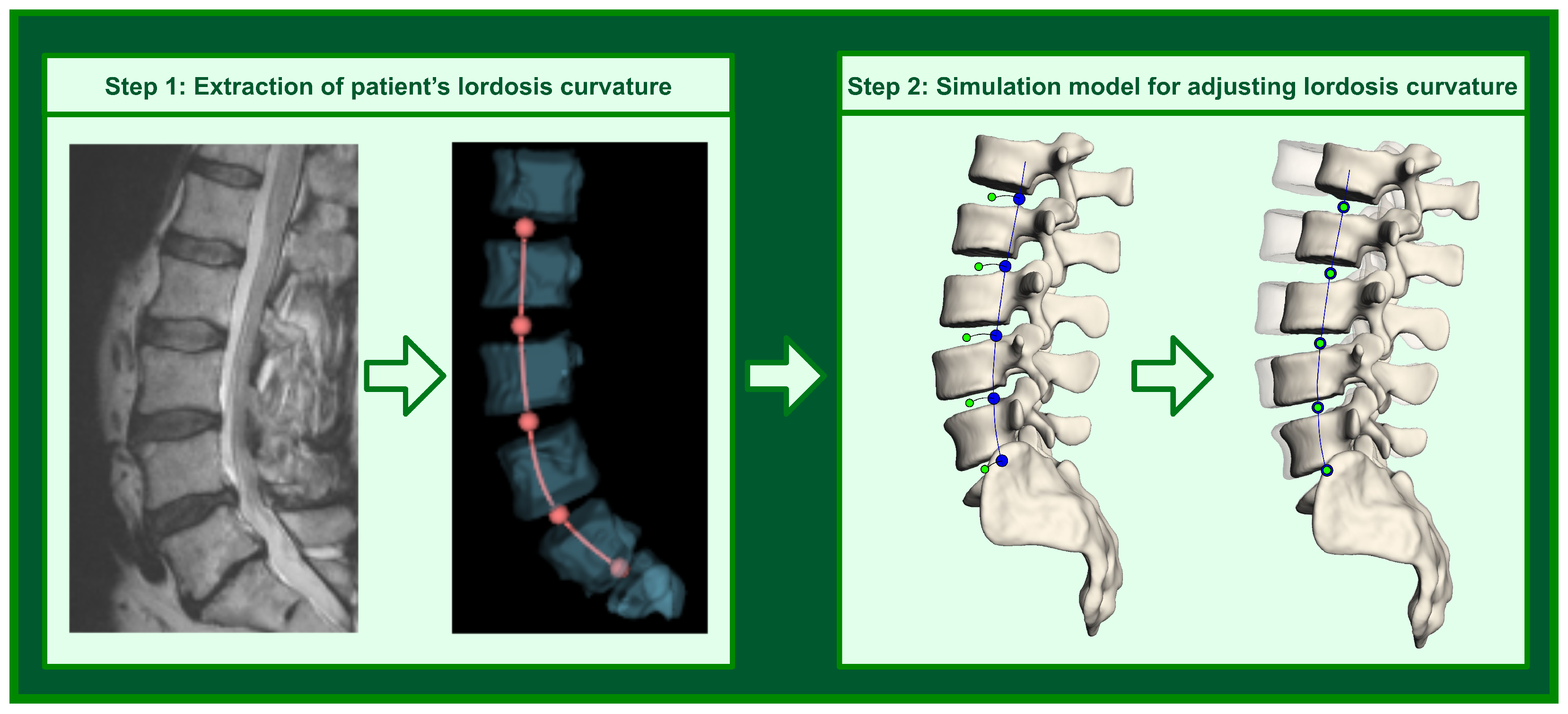
The proposed method includes two steps: extracting the patient’s lordosis curvature from medical data (step 1) and aligning the existing biomechanical spine model to the obtained curvature in the simulation software (step 2). In this section, we show how an individual 3D curve can be derived from 3D vertebral bodies, which are segmented in the spinal magnet resonance images (MRIs) (see Figure 1). Additionally, we explain how the existing spine model is transformed into a new lordosis by applying the obtained lordosis curvature and means of MBS.
2.1. Lordosis Curve Extraction from Medical Data
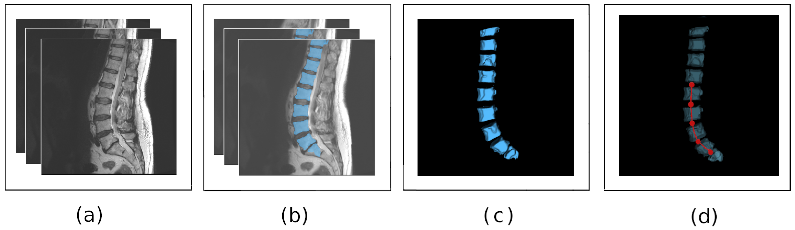
To generate individual lumbar lordosis in the simulation model, a 3D lordosis curve serves as the input. To obtain this 3D curve, medical images can be used. For this purpose, we utilized MRI scans of the lower spine. Furthermore, we trained a deep learning network based on 2D U-Net architecture [12] for the automated localization of the vertebral bodies in the MRI of the lower spine. In the subsequent step, we derived the lordosis curve by fitting the cubic spline through the centers of the segmented 3D vertebral bodies. Four steps of the lordosis curve estimation are depicted in Figure 2a–d.
To train the neural network, we built the training dataset by using publicly available and annotated MR images of the lower spine from different sources. The MyoSegmenTum dataset provided by Burian et al. [13] contains 54 T2*-weighted MRI scans of manually segmented lumbar vertebral bodies (L1 to L5). The dataset released by Zukić et al. [14] includes 17 anonymized MR images of the lower spine (T11 to L5 vertebrae) with the corresponding segmentations. The dataset proposed by Chu et. al. [15] consists of T2-weighted MR spine images of 23 patients, where each image contains at least seven vertebral bodies of the T11–L5 region. Furthermore, we added a custom dataset with MRIs of L5–T10 vertebrae to the training database. Each scan with the volume size around px and image spacing mm contained eight vertebrae from L5 to T10, which we manually segmented and verified through medical experts.
The final dataset resulted in 101 MRI volumes with corresponding annotations, where we randomly selected 70% of the scans for the training and 30% for the validation. We applied Z-score [16] normalization to each of the MRI scans using the mean value of the average pixel intensity of segmented vertebral bodies. Additionally, we applied 0–1 normalization [17], which refers to normalizing the data to approximately the same scale. After that, we extracted 2D sagittal slices from the normalized scans and augmented them. For increased model generalization, we used various augmentation approaches including horizontal flip, elastic transformation [18], translation, scaling, rotation, and the addition of noise. Finally, we interpolated slices to pixels to standardize the neural network input layer.
We trained the neural network model on the lumbar MRI for a maximum of 300 epochs with an initial learning rate of 0.001. To adjust the learning rate based on the relationship between the current epoch number and the maximal count of epochs, we used the PolyLR scheduler proposed by Chen et al. [19].
We trained the neural network on an Nvidia GeForce 2060 RTX GPU with 8192 MB of shader memory. The segmentation result of the trained network is shown in Figure 2a,b. Our implementation of the 2D U-Net is available publicly (https://github.com/VisSim-UniKo accessed on 9 March 2023) and can be used to reproduce the experiments.
In the next step, we derived the 3D lordosis curve by using the segmented vertebral bodies.
To estimate the 3D lordosis curve, we extracted the segmented vertebral bodies (VBs) as 3D volumetric surface meshes (Figure 2c). A 3D lordosis curve was then calculated. To do so, we approximated the lordotic curvature by fitting a cubic spline through the 3D centroids of the segmented VBs. After fitting the curve, the centers of the intervertebral discs as the middle points on the subcurves between the endplates of the adjacent vertebra were determined. In Figure 2d, the estimated curve and the corresponding positions of the intervertebral discs are marked red. Finally, the curve was stored by using 66 points sampled from the fit cubic spline. Hence, the number of the sampled point varies due to the extraction method and can be adopted to the needs of the simulation model. The segments that were considered for the building of the lordosis curvature were the vertebrae from L1 to L5.
2.2. Lordosis Curvature Fitting for Simulation Model
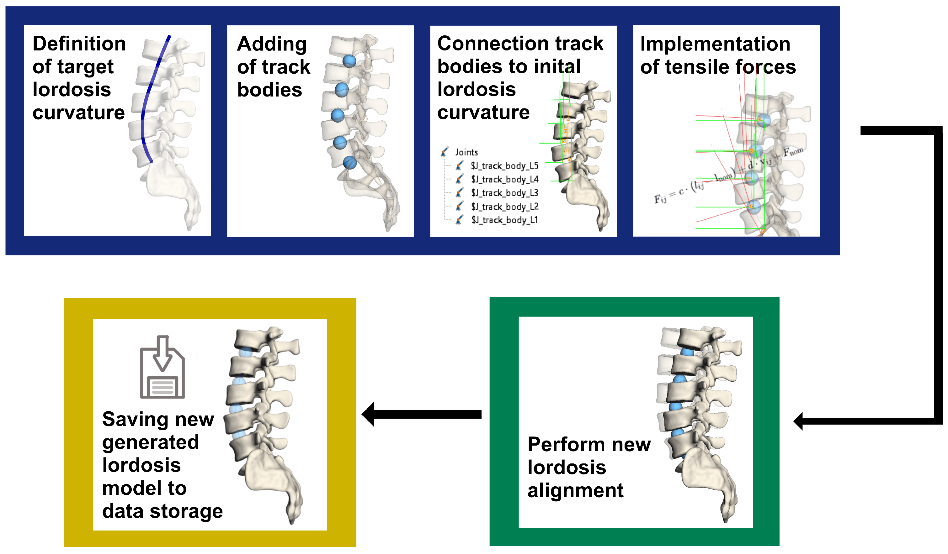
After the 3D lordosis curve is determined from the medical data, it provides the basis in the pipeline for generating a new lordosis in the spine model (Figure 3). The model pipeline consists of three main components: the modeling of the new lordosis (blue), performance of the spine alignment (green), and saving of the generated lordosis models in storage (yellow).
The core aspect of the proposed pipeline is the modeling of the target lordosis curvature. First, the 3D target lordosis curve extracted from the medical image is implemented into the model. In the simulation model, the curve origin is set to the center of the lower endplate of L5. After that, track bodies are created with negligible mass and inertia in the origin of the target intervertebral disc axes of rotation. Thereby, the number of track bodies to be created depends on the model. In our current model, we inserted five track bodies representing five intervertebral discs in the target spine model. In the pipeline depicted in Figure 3, the target lordosis curve is marked dark blue, and the track bodies are visualized by using blue spheres.
By using the track bodies, the entire simulation model with all its components, such as CAD geometries, attachment points for the transmission of ligament and muscle forces, translation and rotation axes of intervertebral discs is transferred to the new positions specified by the target lordosis curvature. To ensure that the defined positions of the track bodies do not deviate from that of the target lordosis curvature, they articulate with this target lumbar curve. It was defined that the track bodies can only move along this predetermined spatial target lordosis curve.
The corresponding intervertebral discs are connected with the associated track bodies by a tensile force. The tensile force can be imagined as a rubber band between a track body and an intervertebral disc, and is implemented as a spring-damper force in the simulation model. The equation describing the tensile force (see Equation (1)) is determined by the stiffness terms , , , , , and damping terms , , . The variable c defines the stiffness and d the damping constants in the three coordinate axis directions. The distance between the center points of the track body and the corresponding intervertebral disc is represented by the variables x, y, and z and the velocity of the interaction points by , , and (see Equation (1)). In the process, each track body pulls the part of the spine connected to it toward itself. As a result of the acting force, all spinal model components are transferred from their initial positions to the new locations so that the lumbar lordosis of the resulting spine model follows the target lordosis curvature, and the position of the intervertebral discs’ centers match the position of the track points along the target curve. We have
The last step of the pipeline is the saving of the new generated lordosis model in storage. The steps described can be repeated if necessary. Any number of models with different lordosis can be made available for simulation. In turn, the effects of these different lordosis may be analyzed in defined simulation scenarios, including dynamic processes such as walking, lifting heavy loads, etc.
3. Results
3.1. Segmentation of Vertebral Bodies from Medical Data
The extraction of the 3D lordosis curve depends on the quality of the segmented vertebral bodies. Therefore, the performance of the trained neural network needed to be evaluated. To validate the segmentation method, we used a confusion matrix and several well-established metrics to describe the relationship between the predicted segmented data and corresponding ground truth. We calculated the metrics on the validation dataset.
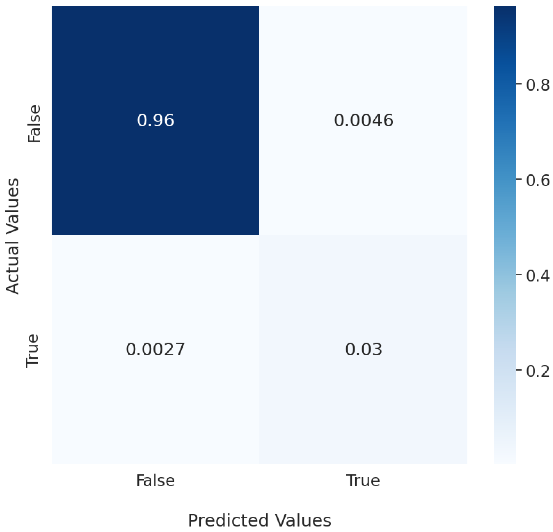
The confusion matrix in Figure 4 shows that the segmentation neural network performed well. The neural network recognized 96% of all segmentation data as true negatives, i.e., regions in the MRI with no vertebral bodies. Furthermore, 3% of the data were correctly predicted by the deep learning model as vertebral bodies. This significant disparity was caused by the high-class imbalance between the foreground, which resembled the lumbar vertebral bodies, and the background. Approximately 0.46% of the background was incorrectly associated with vertebral bodies, whereas 0.27% of vertebral bodies were not recognized as such.
To further evaluate the model performance, we used the accuracy (Acc) and dice score coefficient (DCS) [20]. Accuracy is the ratio between all correctly segmented data to the total segmentations. We have
where TP is the true positive prediction, FP is the false positive prediction, and FN is the false negative prediction. The accuracy of the segmentation result was very high at 99.26%.
To analyze the segmentations in terms of similarity between the annotated and predicted values, we calculated the DSCs:
The neural network achieves a 89.15% DSC. The segmentation result of the trained network is shown in Figure 2b.
3.2. Creation of New Lordosis Model from 3D Curvature
We performed the entire pipeline on three randomly selected patient-specific MRI scans of the lower spine. To determine the degree of lumbar lordosis curve, we used the Cobb angle [21,22], which is a scientifically accepted method from clinical practice. The Cobb angle defines the lumbar lordosis as the sagittal angle between the upper endplate of vertebra L1 and the endplate of the sacrum (Figure 5a). For the measurements, we applied the sagittal image of three different patients and the corresponding generated 3D lumbar spine models. The lordosis values for three selected spines are presented in Table 1.
To ensure that the target lordosis in the simulation model matches the lordosis obtained from the patient data, three independent experts separately annotated the Cobb angles in the MRI data of the three test persons (TPs) as well as in the corresponding generated 3D spine models by using the open-source software 3D Slicer [23] (Figure 5). Furthermore, regarding the interrater reliability of the assigned angle values, we determined a Krippendorff alpha [24] coefficient of .
To determine the error in the degrees between the original and generated lordosis angles, we calculated a mean absolute error (MAE),
where [°] is the lordosis angle measured in the medical image of the patient, [°] is the lordosis angle assigned to the simulation model, and N is the sample size. In our case, we incorporated all raters’ measurements to calculate the MAE, resulting in .
The measured lordosis angle in the medical image and the simulation model showed no significant differences, with an MAE of 1.29. Based on the results presented in Table 1, the mean lordosis angle in the medical images was 44.4° and 44.6° in the simulation model. These values showed that the proposed method could sufficiently reproduce the target lordosis.
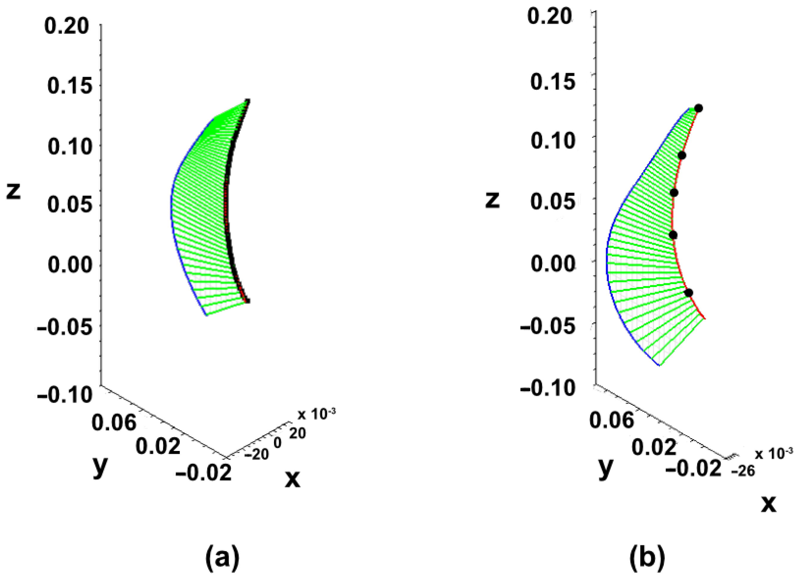
To examine whether the spine in the source simulation model followed the original patient-specific lordosis, we compared the input (Figure 6a) and generated (Figure 6b) lordosis curves. To this end, we analyzed the centroids of five intervertebral disc positions in the newly generated spine model. Of these positions, we approximated the new lordosis curve (Figure 6b).
To quantify the similarity of the original to the target curves, we first calculated the area under the curve (AUC) of the corresponding lordosis curves and then we determined the root mean square error (RMSE) between the corresponding curves. Specifically, we applied the composite Simpson’s formula [25] to estimate the area under the given curve by approximating a value of the definite integral of the function on the interval ,
where and m are the number of subintervals, and a and b are the start and end of the subintervals, respectively. For the required start and end of the integral intervals, we applied the highest and lowest points of the corresponding curves.
Once we determined the AUC values, we used the root mean square error (RMSE) of the validation data to measure the differences between the areas under the given curves (see Equation (6)),
where is the AUC of the target lordosis curve generated in the simulation software, is the area under the original curve derived from medical data of the patient, and N is the number of test samples. This selected metric is commonly used in model evaluation, because it describes the error in units (or squared units) of the component of interest. For simplicity of calculation, we considered the approximated lordosis curves in two planes: sagittal and coronal. Therefore, we needed to determine two RMSE errors: one for the curve in sagittal and one in the coronal axis of the 3D lordosis curve. The results of the RMSE calculation (Table 2) showed a minor difference between the original and generated lordosis curvature areas of 0.0012 m2 in terms of AUC in the sagittal plane (Figure 7a), as well as 0.0001 m2 in the coronal plane (Figure 7b).
The execution time for the two proposed steps of building a new lordosis alignment in the spine model, including the segmentation and generation of the patient-specific curve, was 15 s on an NVIDIA GeForce GTX 1080 Ti with 8 GB VRAM, and up to 25 s wall-clock time for the fitting the target curve in the simulation software (Simpack 2023 (Dassault Systemes Simula GmbH, Germany)) with an Intel(R) Core(TM) i5-5300U CPU @2.30 GHz and four threads. In general, up to 40 s was required for the procedure to transfer the existing generic lumbar spine model to a new lordosis alignment derived from the medical data.
4. Discussion
The adaption of the spinal alignment in the simulation spine models requires an accurate estimation of the patient-specific lordosis curvature in the first step. Nowadays, the patient’s lordosis curve is extracted by using image-processing algorithms and deep learning models on medical images. For example, Grigorieva et al. [26] proposed an approach by which to construct an individualised 3D model of the spine based on X-ray images by using a deep learning convolutional neural network. The 3D spine model was constructed to later determine the extent of scoliosis to design the Cheneau corset. The benefit of our proposed method is, that the 3D target lordosis curve imported into the biomechanical spine model can be extracted from any suitable source of patient data. Therefore, the approach proposed in [26] can be used as an extension of the current method for the further analysis of abnormal spinal curvatures.
Another method that extracts the lumbar lordosis alignment from X-ray data and transfers the lordosis into a simulation model was proposed by Caprara et al. [11]. Combining deep learning techniques with finite element models, they developed a method for generating functional spine units (FSUs). However, compared with their method, our pipeline considers the generation of the the whole lumbar spine model instead of generating only one FSU. To the best of our knowledge, no additional comparable studies exist in the literature with which we could compare our results. If such a method exists in the future, we will validate our proposed method against it.
Our proposed method meets the requirements outlined in the introduction. The current method efficiently extracts the lumbar curvature from medical data without any human effort and then directly transforms the given lordosis into the desired target lordosis alignment in the simulation software. In addition, our method benefits from the MBS, which is more time-efficient than FE simulation [27]. Another fulfilled requirement is that the target lordosis curvature can be taken from any kind of medical data, and the curve can be artificially generated. The method enables a simulation model to use lordosis curvatures from different sources. Furthermore, the extraction of the lordosis curve from medical data and the lordosis curvature fitting for the simulation model can be used as independent steps. Additionally, the proposed method is software-invariant as the lordosis of the spine can be directly adjusted in the simulation model without needing to manually adapt the vertebrae geometries. For the implementation of the spine model in the proposed approach, we used multibody simulation software Simpack 2023 (Dassault Systemes Simula GmbH, Germany). However, other simulation software, e.g., Opensim (https://simtk.org/projects/opensim/ accessed on 9 March 2023) or MATLAB, after a suitable implementation of the tensile force elements was done, can also be applied.
In terms of obtained results, we have shown that the proposed method can precisely reproduce patient-specific lordosis. It is generally accepted that the lower RMSE value indicates better method performance, where a perfect fit is given by the RMSE value of 0. By comparing the RMSE of the areas under the curve in the sagittal and coronal planes of the corresponding lumbar curvatures (Figure 7), we observed negligible deviations between the original and generated lordosis curves in the coronal (0.0001 m2) and sagittal (0.0012 m2) planes. The experimental results showed that the average Cobb angle in the medical data, which was annotated by experts, deviated by 0.2° from the average Cobb angle calculated in the target spinal model. Bassani et al. [28] confirmed that the global sagittal alignment, lumbar typology, and sacral inclination affect the intervertebral loads in the lumbar spine. In future studies, we will clarify to what extent a minor Cobb angle deviation, such as the one given in our method, can affect the spinal load distribution along different vertebral levels.
Supine medical images, such as MRI or CT scans, are commonly used as a valid source in patient-specific modeling because they provide detailed information about the internal structures of the spine, including the vertebrae and intervertebral discs. Therefore, the simulation models created from this data represent the spinal curvature in a supine position. However, the supine position of the spine does not reflect the loads and forces that the spine experiences during upright activities. Suppose the spinal curvature data that differs from the supine position is available in addition to MRI or CT scans. Our method can quickly convert the supine spine model to a standing or situation-adapted spine (target curvature). The target curvature data for this can be obtained from radiographs of a standing person or, for example, by reconstructing the spinal alignment from vision-based measurements [29] of the human back during everyday movements or common postures.
To demonstrate the effectiveness and versatility of the presented pipeline (see Figure 3), we applied the proposed method to standing spine data. To do this, we manually extracted a spinal curvature from a full spine radiograph of a standing person. The initial MBS spine model was then adapted, so that the model lordosis curve matched the input curvature. The input curvature and adapted lumbar spine model are shown in Figure 8. To measure the difference between the adapted curve in the MBS model and the original curve obtained from the radiograph we again calculated the RMSE by setting in sagittal and coronal anatomical planes. Although the full spine curve (C1-Sacrum) was extracted from the radiograph, only the lumbar spine (L1–L5) was considered as an input for the curvature adaption in the MBS model. The difference between the AUC values of the original (taken from the radiograph image) and transformed (from MBS model) lordosis curves is 0.000628 m2 in sagittal and 0.000002 m2 in coronal view correspondingly.
The ability to accurately transform the spinal alignment from a supine to a standing position indicates a high clinical value of the proposed method. Spinal MBS models built from MRI or CT data can be easily extended with appropriate parameters to simulate degenerative processes or surgical procedures such as fusion or implantation. The new knowledge gained from simulation with adjusted spine alignment can provide valuable insight into predicting the load situation of a surgical procedure before it is performed. This preoperative information can then be used to optimize the surgical procedure and improve the clinical outcome for the patient.
In general, demographic information about the patients is not necessary to use our method. In our case, this was not available either. However, patient-specific demographic data can help to draw conclusions about correlations between, e.g., age or lumbar pathology or spinal alignment, and thus should be incorporated in the model generation pipeline in future studies. Furthermore, to advance the building of patient-specific lumbar spine models, the scaling of the initial generic spine model based on the segmented surfaces of the medical images should be incorporated into the proposed pipeline. This feature should also be implemented in the models generating workflow in future studies. Considering the patient-specific characteristics of the spinal structures, such as those of the intervertebral discs, ligaments, etc., individualized therapy and surgery planning can especially benefit from the proposed method.
The load distribution of the spinal structures can then be precisely quantified with patient-specific simulation models. Furthermore, due to the fast and efficient lordosis curvature adaption in the simulation directly, the biomechanical research can benefit from our proposed method in any study that includes the generation of new spinal models. For instance, our approach can be applied in investigating the alternation of the aging lumbar lordosis [30,31] and the consecutive postural changes, which requires implementing multiple patient-specific models for analysis. Additionally, by using our proposed method, researchers can run exhaustive experiments, which may include the generation of new spinal models, thus providing new insights into the mechanism of structural compensations in the spine and throughout the entire body.
5. Conclusions
In this study, we designed a simple and effective method of directly generating a new lordosis alignment in the lumbar spine model in the simulation model without needing to manually adapt the vertebrae alignment. By using this method, the time required for the generation of the new spinal model by an expert, which can take from hours to days depending on the given data and the quality of the segmentation, can be reduced to less than one minute. As a basis for the patient-specific lumbar curvature, we used medical images in this study, which were automatically segmented with a previously trained neuronal network. Then, the lumbar lordosis curvature was approximated by using predicted vertebral bodies. After that, the patient-specific curvature was passed to the simulation model, and five tracking bodies were placed on that curve. Tracking bodies produced a tensile force on the corresponding intervertebral discs and allowed the spine to follow the curvature of the new lordosis alignment. The experimental results show that our proposed approach can be used for the time-efficient generation of MBS spinal models with a defined sagittal alignment.
With the help of the presented method, it is possible to implement the patient-specific alignment of the spine in existing simulation models, and also to convert the prevailing spinal curvature into a different alignment adapted to the movement situation. For example, if in addition to the supine images the curvature of the standing spine can also be included, then the vertebrae in the existing MBS model can be transferred to the new upright alignment.
In conclusion, the proposed approach has been shown to work effectively on different types of data, such as MRI data in a supine position and X-ray data in a standing position, demonstrating the versatility and usefulness of the approach in different applications.
Author Contributions
Methodology, I.K., S.B., and V.K.; validation, I.K. and S.B.; model creation, S.B. and V.K.; automation, script creation: I.K.; writing—original draft preparation: I.K. and S.B.; writing—review and editing: I.K. and S.B.; project administration: I.K. and S.B. All authors have read and agreed to the published version of the manuscript.
Funding
This research was funded by German Federal Ministry of Economic Affairs and Energy, grant number ZF4365203SK9.
Institutional Review Board Statement
The study was conducted in accordance with the Declaration of Helsinki.
Informed Consent Statement
Informed consent was obtained from all subjects involved in the study. Written informed consent has been obtained from the subject to publish this paper.
Data Availability Statement
The medical images used for the training of the deep learning model are publicly available at https://osf.io/3j54b/?view_only=f5089274d4a449cda2fef1d2df0ecc56 accessed on 9 March 2023. Our implementation of the 2D U-Net is available publicly (https://github.com/VisSim-UniKo accessed on 9 March 2023).
Conflicts of Interest
The authors declare no conflict of interest.
Abbreviations
The following abbreviations are used in this manuscript in alphabetical order:
| AUC | Area under the curve |
| CAD | Computer-aided design |
| DCS | Dice score coefficient |
| FE | Finite element |
| LDH | Lumbar disc herniation |
| MAE | Mean absolute error |
| MRI | Magnet resonance images |
| MBS | Multibody simulation |
| RMSE | Root mean square error |
| TP | Test person |
| VB | Vertebral body |
References
- Le Huec, J.C.; Faundez, A.; Dominguez, D.; Hoffmeyer, P.; Aunoble, S. Evidence showing the relationship between sagittal balance and clinical outcomes in surgical treatment of degenerative spinal diseases: A literature review. Int. Orthop. 2014, 39, 87–95. [Google Scholar] [CrossRef]
- Jackson, R.; McManus, A. Radiographic analysis of sagittal plane alignment and balance in standing volunteers and patients with low back pain matched for age, sex, and size. A prospective controlled clinical study. Spine 1994, 19, 1611–1618. [Google Scholar] [CrossRef] [PubMed]
- Boulay, C.; Tardieu, C.; Hecquet, J.; Benaim, C.; Mouilleseaux, B.; Marty, C.; Prat-Pradal, D.; Legaye, J.; Duval-Beaupère, G.; Pélissier, J. Sagittal alignment of spine and pelvis regulated by pelvic incidence: Standard values and prediction of lordosis. Eur. Spine J. Off. Publ. Eur. Spine Soc. Eur. Spinal Deform. Soc. Eur. Sect. Cerv. Spine Res. Soc. 2006, 15, 415–422. [Google Scholar] [CrossRef] [PubMed] [Green Version]
- Legaye, J.; Duval-Beaupère, G. Sagittal plane alignment of the spine and gravity A radiological and clinical evaluation. Acta Orthop. Belg. 2005, 71, 213–220. [Google Scholar] [PubMed]
- Hasegawa, K.; Okamoto, M.; Hatsushikano, S.; Caseiro, G.; Watanabe, K. Difference in whole spinal alignment between supine and standing positions in patients with adult spinal deformity using a new comparison method with slot-scanning three-dimensional X-ray imager and computed tomography through digital reconstructed radiography. BMC Musculoskelet. Disord. 2018, 19, 437. [Google Scholar] [CrossRef] [PubMed]
- Lee, E.S.; Ko, C.W.; Suh, S.W.; Kumar, S.; Kang, I.K.; Yang, J.H. The effect of age on sagittal plane profile of the lumbar spine according to standing, supine, and various sitting positions. J. Orthop. Surg. Res. 2014, 9, 11. [Google Scholar] [CrossRef] [PubMed] [Green Version]
- Beck, J.; Brisby, H.; Baranto, A.; Westin, O. Low lordosis is a common finding in young lumbar disc herniation patients. J. Exp. Orthop. 2020, 7, 38. [Google Scholar] [CrossRef]
- Bassani, T.; Ottardi, C.; Costa, F.; Brayda-Bruno, M.; Wilke, H.J.; Galbusera, F. Semiautomated 3D Spine Reconstruction from Biplanar Radiographic Images: Prediction of Intervertebral Loading in Scoliotic Subjects. Front. Bioeng. Biotechnol. 2017, 5, 1. [Google Scholar] [CrossRef] [Green Version]
- Fasser, M.R.; Jokeit, M.; Kalthoff, M.; Gomez Romero, D.A.; Trache, T.; Snedeker, J.G.; Farshad, M.; Widmer, J. Subject-Specific Alignment and Mass Distribution in Musculoskeletal Models of the Lumbar Spine. Front. Bioeng. Biotechnol. 2021, 9, 745. [Google Scholar] [CrossRef]
- Mueller, A.; Rockenfeller, R.; Damm, N.; Kosterhon, M.; Kantelhardt, S.R.; Aiyangar, A.K.; Gruber, K. Load Distribution in the Lumbar Spine During Modeled Compression Depends on Lordosis. Front. Bioeng. Biotechnol. 2021, 9, 661258. [Google Scholar] [CrossRef]
- Caprara, S.; Carrillo, F.; Snedeker, J.G.; Farshad, M.; Senteler, M. Automated Pipeline to Generate Anatomically Accurate Patient-Specific Biomechanical Models of Healthy and Pathological FSUs. Front. Bioeng. Biotechnol. 2021, 9, 636953. [Google Scholar] [CrossRef]
- Ronneberger, O.; Fischer, P.; Brox, T. U-net: Convolutional networks for biomedical image segmentation. In Proceedings of the International Conference on Medical Image Computing and Computer-Assisted Intervention, Munich, Germany, 5–9 October 2015; Springer: Berlin/Heidelberg, Germany, 2015; pp. 234–241. [Google Scholar]
- Burian, E.; Rohrmeier, A.; Schlaeger, S.; Dieckmeyer, M.; Diefenbach, M.; Syväri, J.; Klupp, E.; Weidlich, D.; Zimmer, C.; Rummeny, E.; et al. Lumbar muscle and vertebral bodies segmentation of chemical shift encoding-based water-fat MRI: The reference database MyoSegmenTUM spine. BMC Musculoskelet. Disord. 2019, 20, 152. [Google Scholar] [CrossRef] [PubMed]
- Zukić, D.; Vlasák, A.; Egger, J.; Hořínek, D.; Nimsky, C.; Kolb, A. Robust detection and segmentation for diagnosis of vertebral diseases using routine MR images. In Proceedings of the Computer Graphics Forum; Wiley Online Library: Hoboken, NJ, USA, 2014; Volume 33, pp. 190–204. [Google Scholar]
- Chu, C.; Belavỳ, D.L.; Armbrecht, G.; Bansmann, M.; Felsenberg, D.; Zheng, G. Fully automatic localization and segmentation of 3D vertebral bodies from CT/MR images via a learning-based method. PLoS ONE 2015, 10, e0143327. [Google Scholar] [CrossRef] [PubMed] [Green Version]
- LeCun, Y.A.; Bottou, L.; Orr, G.B.; Müller, K.R. Efficient backprop. In Neural Networks: Tricks of the Trade; Springer: Berlin/Heidelberg, Germany, 2012; pp. 9–48. [Google Scholar]
- Gopal Krishna Patro, S.; Sahu, K.K. Normalization: A Preprocessing Stage. arXiv 2015, arXiv:1503.06462. [Google Scholar]
- Simard, P.Y.; Steinkraus, D.; Platt, J.C. Best practices for convolutional neural networks applied to visual document analysis. In Proceedings of the Seventh International Conference on Document Analysis and Recognition, Edinburgh, UK, 3–6 August 2003; pp. 958–963. [Google Scholar] [CrossRef]
- Chen, L.C.; Papandreou, G.; Kokkinos, I.; Murphy, K.; Yuille, A.L. Deeplab: Semantic image segmentation with deep convolutional nets, atrous convolution, and fully connected crfs. IEEE Trans. Pattern Anal. Mach. Intell. 2017, 40, 834–848. [Google Scholar] [CrossRef] [PubMed] [Green Version]
- Sørenson, T. A Method of Establishing Groups of Equal Amplitude in Plant Sociology Based on Similarity of Species Content and Its Application to Analyses of the Vegetation on Danish Commons; Royal Danish Academy of Sciences and Letters: Copenhagen, Denmark, 1948. [Google Scholar]
- Furlanetto, T.; Sedrez, J.; Candotti, C.; Loss, J. Reference values for Cobb angles when evaluating the spine in the sagittal plane: A systematic review with meta-analysis. Motricidade 2018, 14, 115–128. [Google Scholar] [CrossRef] [Green Version]
- Comparison of Four Radiographic Angular Measures of Lumbar Lordosis. J. Neurosci. Rural Pract. 2018, 9, 298–304. [CrossRef] [Green Version]
- Kikinis, R.; Pieper, S.D.; Vosburgh, K.G. 3D Slicer: A Platform for Subject-Specific Image Analysis, Visualization, and Clinical Support. In Intraoperative Imaging and Image-Guided Therapy; Jolesz, F.A., Ed.; Springer: New York, NY, USA, 2014; pp. 277–289. [Google Scholar] [CrossRef]
- Hayes, A.F.; Krippendorff, K. Answering the call for a standard reliability measure for coding data. Commun. Methods Meas. 2007, 1, 77–89. [Google Scholar] [CrossRef]
- Young, D.M.; Gregory, R.T. A Survey of Numerical Mathematics; Courier Corporation: North Chelmsford, MA, USA, 1988; Volume 1. [Google Scholar]
- Grigorieva, I.; Vyunnik, N.; Kolpinsky, G. The Construction of an Individualized Spinal 3D Model Based on the X-ray Recognition. In Proceedings of the 2018 23rd Conference of Open Innovations Association (FRUCT), Bologna, Italy, 13–16 November 2018; IEEE: Helsinki, Finland; pp. 143–149. [Google Scholar] [CrossRef]
- Bauer, S. Basics of Multibody Systems: Presented by Practical Simulation Examples of Spine Models. In Numerical Simulation; Lopez-Ruiz, R., Ed.; IntechOpen: Rijeka, Croatia, 2016; Chapter 2. [Google Scholar] [CrossRef] [Green Version]
- Bassani, T.; Casaroli, G.; Galbusera, F. Dependence of lumbar loads on spinopelvic sagittal alignment: An evaluation based on musculoskeletal modeling. PLoS ONE 2019, 14, e0207997. [Google Scholar] [CrossRef] [Green Version]
- Krautwurst, B.K.; Paletta, J.R.; Mendoza, S.; Skwara, A.; Mohokum, M. Rasterstereographic Analysis of Lateral Shift in Patients with Lumbar Disc Herniation: A Case Control Study. Adv. Orthop. 2018, 2018, 6567139. [Google Scholar] [CrossRef] [Green Version]
- Shirazi-Adl, A.; Parnianpour, M. Effect of changes in lordosis on mechanics of the lumbar spine-lumbar curvature in lifting. J. Spinal Disord. 1999, 12, 436–447. [Google Scholar] [CrossRef] [PubMed]
- Coskun Benlidayi, I.; Basaran, S. Comparative study of lumbosacral alignment in elderly versus young adults: Data on patients with low back pain. Aging Clin. Exp. Res. 2015, 27, 297–302. [Google Scholar] [CrossRef] [PubMed]
Figure 1.
Representation of the method’s pipeline containing two substeps for an automatic adjustment of the lumbar curvature alignment in a spine model. In the preprocessing step, the patient-specific lumbar curvature is extracted from medical data. The fitting of the lumbar lordosis to the patient-specific spinal curvature in the simulation model is completed in the subsequent step.

Figure 2.
Extraction of lordosis curve from patient data image. (a) An input MR image of subject is segmented by using a neural network. Vertebral bodies (b) are localized in each slide of the given MRI. The segmented vertebral bodies are marked blued in the sample slice. In the consecutive step (c), volumetric surface meshes are generated from the 2D segmented slices in order to estimate a 3D lumbar curve. In the last step (d), a 3D curve is fitted through 3D vertebral bodies (L1–L5). The centroids of the corresponding intervertebral discs, which are used in the next phase of the proposed approach, are represented by red spheres.

Figure 3.
Pipeline of the adaption from the initial to the target lordosis. The blue box shows the preprocessing step of the data. This step includes the definition of the target lordosis curvature (marked as a blue curve), the adding of the track bodies (light blue spheres), the connection of the track bodies to the target lordosis curvature, and the implementation of the tensile forces. The next step of the pipeline is the performance of the new lordosis alignment presented in the green box. The transparent geometries belong to the initial model and the solid to the target model. The final pipeline step is the saving of the new generated lordosis model represented in the yellow box.

Figure 4.
Confusion matrix representing actual and predicted values of the trained neural network.

Figure 5.
Example comparison of lordosis determined from medical image and simulation model. (a) Sagittal image taken from patient MRI. (b) Target lumbar spine model with generated lordosis.
Figure 5.
Example comparison of lordosis determined from medical image and simulation model. (a) Sagittal image taken from patient MRI. (b) Target lumbar spine model with generated lordosis.

Figure 6.
Example of the lordosis curves generated for the test person 2 (TP2) in different anatomical planes. (a) Curves in sagittal plane. (b) The lordosis curves in coronal plane. The area under the curve is marked transparent.
Figure 6.
Example of the lordosis curves generated for the test person 2 (TP2) in different anatomical planes. (a) Curves in sagittal plane. (b) The lordosis curves in coronal plane. The area under the curve is marked transparent.

Figure 7.
Sample input and generated lordosis curves. (a) Curve approximated as cubic spline through 66 sampled points (marked in black) from patient MR image. (b) Lordosis curve (marked in red) from newly generated spine model and approximated by using five points (marked in black) that represent centers of intervertebral discs in generated simulation spine model.

Figure 8.
Full spine radiographs of a standing person taken with the EOS medical imaging system. (a) Lateral EOS image of a person with patient-specific spinal alignment. (b) The spinal curve is fitted through the 3D vertebral bodies of the C1-Sacrum and the corresponding intervertebral discs. For the generation of a new lordosis in the MBS model, the sub-curve L1-Sacrum was applied as an input to the transformation pipeline, (c) the corresponding MBS-model with the new adapted lordosis alignment. The curve extracted from the radiograph image (marked purple) is used at this place for visualization purposes only.


Table 1.
Cobb angle (in ) measured in medical images (MRI) of different test persons and corresponding simulation models (Sim).
Table 1.
Cobb angle (in ) measured in medical images (MRI) of different test persons and corresponding simulation models (Sim).
| Test Person | Rater 1 [] | Rater 2 [] | Rater 3 [] | Mean [] | SD [] |
|---|---|---|---|---|---|
| 33.8 | 33.8 | 33.7 | 33.8 | 0.057 | |
| 34.0 | 33.5 | 34.5 | 34.0 | 0.5 | |
| 45.5 | 45.4 | 45.3 | 45.4 | 0.1 | |
| 47.5 | 46.4 | 47.2 | 47.0 | 0.6 | |
| 52.3 | 52.8 | 57.1 | 54.1 | 2.6 | |
| 52.9 | 52.8 | 52.7 | 52.8 | 0.3 |
Table 2.
Root mean square error (RMSE) of the area under the curve of the generated curve in the simulation model and patient-specific curve.
Table 2.
Root mean square error (RMSE) of the area under the curve of the generated curve in the simulation model and patient-specific curve.
| [] | [] |
|---|---|
| 0.0012 | 0.0001 |
Disclaimer/Publisher’s Note: The statements, opinions and data contained in all publications are solely those of the individual author(s) and contributor(s) and not of MDPI and/or the editor(s). MDPI and/or the editor(s) disclaim responsibility for any injury to people or property resulting from any ideas, methods, instructions or products referred to in the content. |
© 2023 by the authors. Licensee MDPI, Basel, Switzerland. This article is an open access article distributed under the terms and conditions of the Creative Commons Attribution (CC BY) license (https://creativecommons.org/licenses/by/4.0/).
Share and Cite
MDPI and ACS Style
Kramer, I.; Bauer, S.; Keppler, V. A Simple, Efficient Method for an Automatic Adjustment of the Lumbar Curvature Alignment in an MBS Model of the Spine. Biomechanics 2023, 3, 166-180. https://doi.org/10.3390/biomechanics3020015
AMA Style
Kramer I, Bauer S, Keppler V. A Simple, Efficient Method for an Automatic Adjustment of the Lumbar Curvature Alignment in an MBS Model of the Spine. Biomechanics. 2023; 3(2):166-180. https://doi.org/10.3390/biomechanics3020015
Chicago/Turabian StyleKramer, Ivanna, Sabine Bauer, and Valentin Keppler. 2023. "A Simple, Efficient Method for an Automatic Adjustment of the Lumbar Curvature Alignment in an MBS Model of the Spine" Biomechanics 3, no. 2: 166-180. https://doi.org/10.3390/biomechanics3020015