An Overview of Selected Material Properties in Finite Element Modeling of the Human Femur

Abstract

Specific finite detail modeling of the human body gives a capable primary enhancement to the prediction of damage risk through automobile impact. Currently, car crash protection countermeasure improvement is based on an aggregate of testing with installed anthropomorphic test devices (i.e., ATD or dummy) and a mixture of multibody (dummy) and finite element detail (vehicle) modeling. If an incredibly easy finite element detail version can be advanced to capture extra statistics beyond the abilities of the multi-body structures, it might allow advanced countermeasure improvement through a more targeted prediction of overall performance. Numerous research has been done on finite element analysis of broken femurs. However, there are two missing pieces of information: 1- choosing the right material properties, and 2- designing a precise model including the inner structure of the bone. In this research, most of the chosen material properties for femur bone will be discussed and evaluated.

1. Introduction

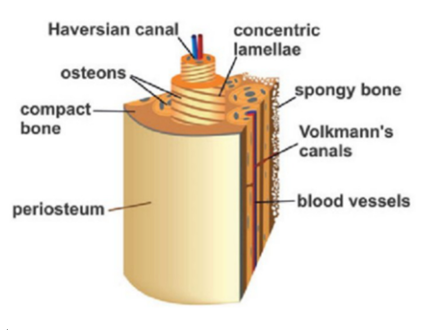
Finite element analysis has a large number of usages in medical, agricultural, and mechanical products [1,2]. Finite element modeling of the human femur, like most biological structures [3], has an inherent challenge in that building a material model capable of describing the two complex bone tissues [4], cortical and cancellous, is extremely worrying. Consequently, the development of any such finite element model requires a whole lot of extra time,- and the level of expertise in non-linear material continuum mechanics required to enhance correct fabric model descriptions is a good deal higher. This caveat necessitates the significance of investigating whether this excessive degree of material model complexity (in particular in the anisotropic description) is essential. The human femur has, via numerous investigations, been physically examined (e.g., examining a human cadaver with complete bones) yielding knowledge on obvious complete bone structures (e.g., whole bone stiffness and elastic bending) [5,6,7,8,9,10]. It has also been digitized and modeled in lots of distinct finite element applications both at the tissue level and at the complete bone macroscopic level [11,12,13,14,15]. Lots of designs have additionally been achieved to ascertain the femur bone tissue materials’ (cortical and cancellous) linear and non-linear material properties by way of methods starting from mechanical and acoustic testing to more theoretical ways [14,16,17,18,19,20,21,22,23,24]. The more accurate finite element (FE) design of the femur entire bone, or, separately, the bone tissues, encompass a fabric design that describes a few grades of fabric anisotropy, or specific directional conduct [25], in addition to pressure dependence. As shown in Figure 1, there are a colossal number of sections inside a bone that contain marrow, trabeculae, Haversian canals, etc. [26]. Most of the researchers conducted FE analysis on the fractured femur with standard triangle language (STL) files of the human femur fixed with different types of implants (dynamic hip screws (DHS), cannulated screws (CS), etc.) [27,28,29,30,31]. Therefore, researchers are unable to design a model of a human femur with this approach. Most of them used the STL file of the human femur, which is converted from a computerized tomography (CT scan) file. Therefore, it is impossible to edit or change the STL file of the model. Some of them designed a simplified model of the human femur, leaving out certain parts of the femur [2]. In this research, three sections of the bone (cortical, trabeculae, and marrow) with three types of material (isotropic, anisotropic, and orthotropic) were discussed, and the approach of defining them in Ansys is explained. In the following parts, different types of material will be illustrated step by step. The aim of this research is to help other researchers to use the right material properties of the femur bone and obtain accurate results.

1.1. Types of Material Properties

This section demonstrates the major types of material properties (isotropic, anisotropic, and orthotropic), which were used in FE analysis of the human femur and will be introduced precisely.

1.1.1. Isotropic Materials

Isotropic materials have similar physical and mechanical properties in all directions. The identical strength, stress, strain, young’s modulus, and hardness of isotopic materials will be evaluated when a selected load is carried out at any point inside the x, y, or z-axis. Additionally, isotropic material does not have a dependency on the direction that light travels. It has just a deflection index. The deflection index is the ratio of light speed in a vacuum to the phase rate in a material through which light moves. So, light speed in isotopic materials is not impacted by the varying direction of irradiation. The elastic Young’s modulus (E) and Poisson’s ratio (v) are the main properties that were used for femur analysis with isotropic material. They show material stiffness and the ratio of lateral strain to axial strain, respectively [32].

1.1.2. Anisotropic Materials

Anisotropic materials, additionally mentioned as “triclinic” materials, depend on directions that are made from the unsymmetrical crystalline structure. In other words, there is a relation between the mechanical behavior of anisotropic materials and the orientation of the material’s body. When the same load is applied to various axes, each surface responds differently. This suggests that measurements of a particular mechanical or thermal property taken along the x-axis will be different from measurements taken along the y-axis or z-axis. Additionally, regarding reference axes, there are differences in the concentration and distribution of atoms. Therefore, the measurements also change as the axis does. There are five independent properties in anisotropic material including two Young’s moduli, E1 (principal modulus) and E3 (or E2, modulus in the transverse plane); two shear moduli, G12 (or G13) and G23; and one Poisson ratio, v. anisotropy. In physics, the quality of exhibiting properties with different values is measured along axes in different directions. Anisotropy is most easily observed in single crystals of solid elements or compounds, in which atoms, ions, or molecules are arranged in regular lattices. [33].

1.1.3. Orthotropic Materials

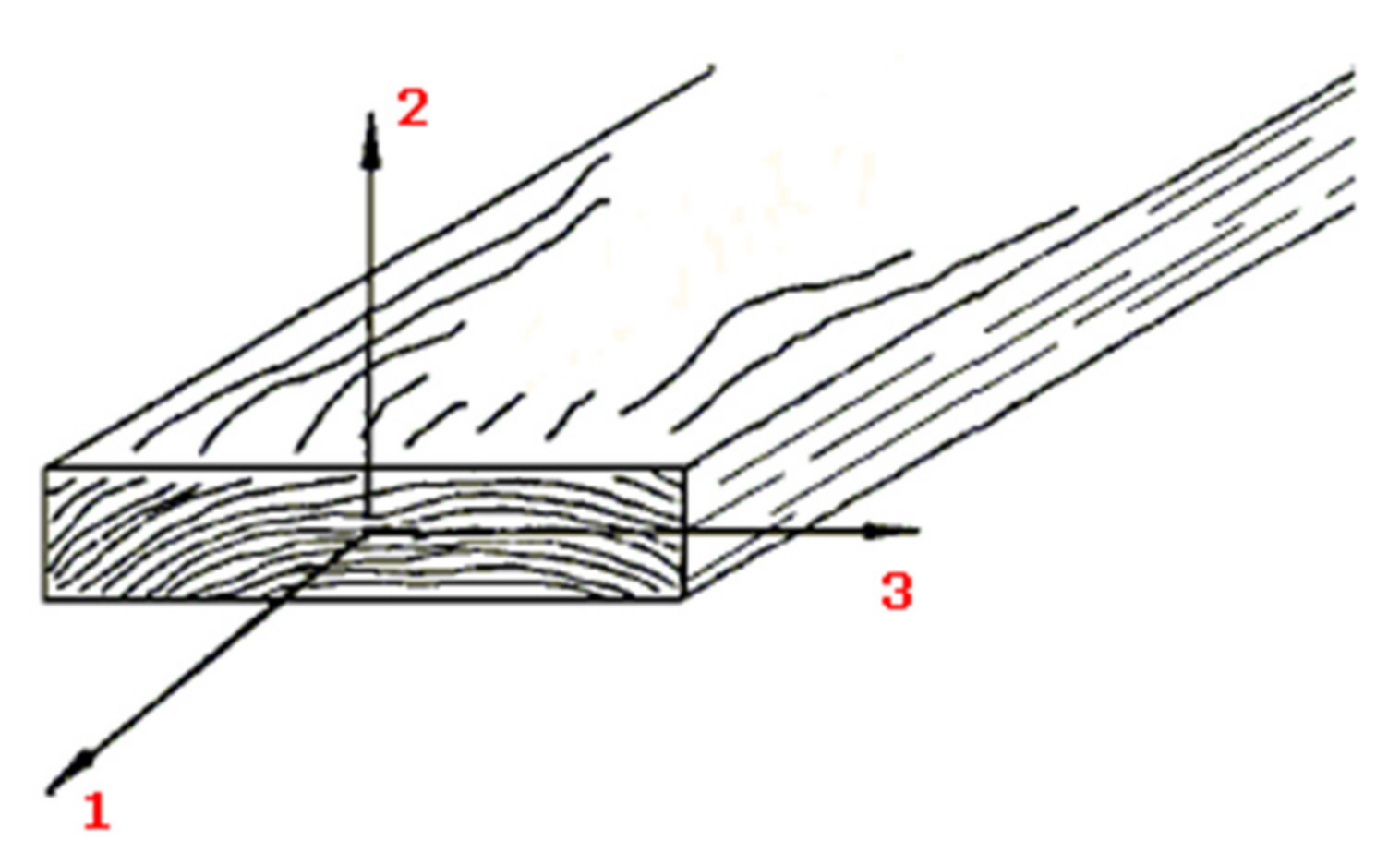
If a material exhibits distinct and independent mechanical or thermal characteristics in three mutually perpendicular directions, it is said to be orthotropic. Wood, many crystals, and rolling metals are a few examples of orthotropic materials. For instance, the longitudinal, radial, and tangential directions are used to explain the mechanical characteristics of wood at a place. The radial axis (2) is normal, while the longitudinal axis (1) is parallel to the direction of the grain (fiber); the radial axis (2) is normal to the growth rings, and the tangential axis (3) is tangent to the growth rings (Figure 2). There are nine independent material properties that entail Young’s moduli in three directions (E1, E2, and E3), a trio of shear moduli (G12, G13, and G23), and three Poisson’s ratios (v12, v13, and v23) [34]. These are limited in a thermodynamically constant material.

E₁, E₂, E₃, G₁₂, G₂₃, G₃₁ >0

(1)

C₁₁, C₂₂, C₃₃, C₄₄, C₅₅, C₆₆ > 0

(2)

(1 − U₂₃ U₃₂). (1 − U₁₃ U₃₁). (1 − U₁₂ U₂₁) > 0

(3)

1 − (U₁₂ U₂₁) − (U₂₃ U₃₂) − (U₃₁ U₁₃) − 2(U₂₁ U₃₂ U₁₃) > 0

(4)

Also, by symmetry,

$${\nu }_{ji}={\nu }_{ij} \frac{E_{jj}}{E_{ii}}$$

(5)

Equations (2) and (5) create the conditions shown below.

$$\left|{\nu }_{21}\right|\le {\left. [\frac{E_{22}}{E_{11}}\right]}^{\frac{1}{2}}, \left|{\nu }_{12}\right|\le {\left. [\frac{E_{11}}{E_{22}}\right]}^{\frac{1}{2}}, \left|{\nu }_{132}\right|\le {\left. [\frac{E_{33}}{E_{22}}\right]}^{\frac{1}{2}}$$

$$\left|{\nu }_{23}\right|\le {\left. [\frac{E_{22}}{E_{33}}\right]}^{\frac{1}{2}}, \left|{\nu }_{31}\right|\le {\left. [\frac{E_{33}}{E_{11}}\right]}^{\frac{1}{2}}, \left|{\nu }_{13}\right|\le {\left. [\frac{E_{11}}{E_{33}}\right]}^{\frac{1}{2}}$$

With the selection of the material parameters used in this investigation, Equation (1) is satisfied. Both trabeculae and cortical bone’s material qualities meet the requirements of Equations (3)–(5).

1.2. Physical and Mechanical Properties of the Human Femur

Data from mechanical tensile tests were used where they were pertinent to the circumstances of this study. Not every range given in the literature applies to all of the material constants utilized in this investigation. This difference is to be expected given many factors, such as age, pathology, and sample size. To give the material models’ average properties, tabulated tissue response data and average values from several investigations are employed whenever practical. The specific material inputs selected for each material model are shown in this section. For the sake of model simplicity, the separate bone tissues are also given a uniform apparent density throughout the femur of 1.9 g/cm³ for cortical tissue and 0.4 g/cm³ for trabecular tissue. This is in addition to the mechanical properties indicated.

1.2.1. Material Properties for Trabeculae

Elected orthotropic material qualities are listed in

Table 1. Trabeculae as orthotropic material.

Young’s Moduli (MPa)	Shear Moduli (MPa)	Poisson’s Ratios
E1 = 1352	G12 = 292	V12 = 0.30
E2 = 968	G23 = 370	V23 = 0.30
E3 = 676	G13 = 505	V13 = 0.30

. The following criteria guided the selection of these:

• All orthogonal moduli are comparable to values published in [35] and [23] and fall within the generally accepted range of 0–4.74 GPa [24].
• For cancellous bone tissue, the ratios of the directional Young’s moduli exhibit a relationship similar to that reported in [36], where E₁/E₂ and E₁/E₃ are equal to approximately 2 (here, equal to 1.4 and 2.0, respectively), and E₃/E₂ is equal to approximately 0.6 (here, 0.07).
• The typical Young’s modulus is 1.0 GPa, which is in accordance with what has been documented in the literature.

The selected isotropic and anisotropic material properties for cancellous bone are shown in

Table 2. Trabeculae as anisotropic material.

Young’s Moduli (MPa)	Shear Moduli (MPa)	Poisson’s Ratios
E1 = 1352	G12 = 399	V12 = 0.30
E2 = 822	G23 = 370	V23 = 0.30
E3 = 822	G13 = 399	V13 = 0.30

and

Table 3. Trabeculae as isotropic material.

Young’s Moduli (GPA)	Poisson’s Ratios
E1 = 1	V12 = 0.30

. Notably, the shear moduli in planes 1–3 and 1–2 were averaged to 399 MPa for the transversely isotropic material model, whereas the moduli in the second and third directions were 822 MPa on average. The average Young’s modulus and average Poisson’s ratio for the isotropic model are 1.0 GPa and 0.3, respectively.

The inputs for the isotropic piecewise linear plasticity material model of cancellous bone are displayed in

Table 4. Trabeculae as a nonlinear isotopic model.

Elastic Modulus (MPa)	Tangent Modulus (MPa)	Poisson’s Ratios	Yield Stress (MPa)
E = 1000	Etan = 1000	0.3	7.5

. According to [20], the tangent modulus is set at 5% of the elastic modulus. The yield stress is the average of the values for the greater trochanter and femoral neck described in [24], which is roughly 3 MPa and 12 MPa, respectively.

1.2.2. Material Properties for Cortical Bone

Two of the few researchers that have looked into the directional moduli of cortical bone are Reilly and Burnstein [17]. The results are mentioned below:

E₁ = 8.69 GPa (longitudinal), E₂ = 4.19 GPa (transverse), and E₃ = 3.76 GPa (radial).

The following ratios, presented as approximate percentages, can be extracted from the data, despite the fact that this E₁ is substantially lower than that of the majority of other studies: E₂/E₁ = 48%, E₃/E₂ = 90%, and E₃/E₁ = 43%. The longitudinal tensile and bending moduli for wet human cortical bone specimens, principally from the femur, are listed in detail in

Table 5. Cortical bone as an orthotropic material.

Young’s Moduli (GPa)	Shear Moduli (GPa)	Poisson’s Ratios
E1 = 16	G12 = 3.2	V12 = 0.30
E2 = 6.88	G23 = 3.6	V23 = 0.45
E3 = 6.30	G13 = 3.3	V13 = 0.30

[18]. As can be observed, the average longitudinal Young’s modulus throughout these experiments is 16.0 GPa. Using the aforementioned percentages, E₂ and E3 are equivalent to roughly 6.8 GPa and 6.3 GPa, respectively, with E1 equal to 16.0 GPa. Shear moduli are found in Schuster [11] and are comparable to an average shear modulus of 3.36 GPa as reported by Reilly and Burnstein [17]. In another study, Mirzaali et al. [37] evaluated the physical and mechanical properties of cortical bone in different cases. It was written that the axial hardness modulus for osteonal, interstitial, and pooled bone are 408 ± 69, 503 ± 56, and 455 ± 78, respectively. Therefore, transverse hardness moduli for female, male, and pooled bone are 367 ± 91, 428 ± 75, and 395 ± 89 respectively. In uniaxial tests, the moduli are 18.16 ± 1.88 and 18.97 ± 1.84 under uniaxial tension and compression, respectively. The Poisson’s ratios for cortical tissue recorded by Reilly and Burnstein [17] were 0.62 for “radial specimens” and 0.40 for “longitudinal specimens”. Since Poisson ratios greater than 0.5 are not permitted in the infinitesimal theory, these values led to problems in the constitutive equations used for the orthotropic material model. As a result, the ratios were reduced while maintaining their relative magnitudes. The radial and longitudinal Poisson’s ratios are scaled to 0.45 and 0.30, respectively. These are comparable to the average Poisson’s ratio for femoral cortical bone tissue reported by Katsamanis and Raftopoulos [38] of 0.36. The transverse direction of Poisson’s ratio in this study is also calculated using the Poisson’s ratio for the radially harvested specimen (set to 0.3).

Table 6. Cortical bone as an anisotropic material.

Young’s Moduli (GPa)	Shear Moduli (GPa)	Poisson’s Ratios
E1 = 16	G12 = 3.3	V12 = 0.30
E2 = 6.30	G23 = 3.6	V23 = 0.45
E3 = 6.30	G13 = 3.3	V13 = 0.30

lists the final nine elastic material constants used for the orthotropic cortical bone. The orthotropic material model description with E₂ = E₃ = 6.30 GPa and G₁₂ = G₁₃ = 3.30 is all that is required to describe the transversely isotropic material model for cortical tissue, as illustrated in

Table 7. Cortical bone as an isotropic material.

Young’s Moduli (GPa)	Poisson’s Ratios
E1 = 16	V12 = 0.36

.

Table 8. Cortical bone as a nonlinear isotopic model.

Elastic Modulus (GPa)	Tangent Modulus (MPa)	Poisson’s Ratios	Yield Stress (MPa)
E = 16	Etan = 800	0.36	108

displays the isotropic material model description for cortical tissue. The material constants for the isotropic piecewise linear- plasticity material model of cortical bone are displayed in

Table 9. Effective Young’s Modulus comparisons for samples from the same bone using in vitro methods.

Marrow Sample Temperature	Rheology (kPa)	Indentation (kPa)	Cavitation (kPa)
	25 °C	20 °C	20 °C
1	52.1 ±10.2	30.3 ± 4.0	64.3 ± 0.2
2	4.0 ± 0.9	5.7 ± 0.3	9.0 ± 0.01
3	0.7 ± 0.3	0.9 ± 0.2	0.9 ± 0.2
4	3.2 ± 1.9	2.1 ± 0.3	14.4 ± 10.0
5	84.4 ± 6.5	35.3 ± 4.9	no data
6	135.6 ± 25.6	37.1 ± 6.3	no data
7	69.0 ± 21.4	—	—
8	—	12.2 ± 2.8	—
9	—	—	16.0 ± 1.6
Average	38.77	13.73	11.52

. The yield stress is the average of the tension values for specimens tested in by Reilly and Burnstein [17], and the elastic modulus and Poisson’s ratio are the same used for the elastic isotropic model. The tangent modulus is 5% of the elastic modulus [20].

1.2.3. Material Properties for Marrow

In comparison to past investigations, our data on bone marrow mechanics are both substantially stiffer and cover a wider range of values. However, as was already mentioned, other studies have used homogenized tissue samples, so it is difficult to compare the reported viscosities, which range from 44.6 to 142 mPas, with our data, which range from 100 to 500 Pa. [38,39,40,41,42,43]. At physiological marrow temperature (35 °C), intact bone marrow tissue has an effective Young’s modulus range from 0.25–24.7 kPa (Table 9). Bovine bone marrow has a dynamic storage modulus of about 220 Pa at a frequency of 1.6 Hz and a temperature of 37 °C, according to the only other study on the rheology of intact marrow [44]. Our porcine samples had a dynamic storage modulus ranging from 23–10,000 Pa at this same frequency but at 35 °C (data not shown). Although their effort was limited to three samples from the same bone, this hindered their ability to detect biological heterogeneities in marrow samples. Nevertheless, this study is consistent with the storage magnitude we find for intact marrow. Because biological tissues are known to be diverse, it is not surprising that we discovered intact marrow to exhibit a significant level of inter-sample heterogeneity. For instance, reports on the elastic modulus of lung and brain tissue have been found to range from 1.5 to 100 kPa and 0.1 to 10 kPa, respectively [43,45,46,47,48,49,50]. It was crucial to confirm that the variety of mechanical tests employed to collect these data was not the source of this heterogeneity, as we have done here, even though it is more plausible that these variances are caused by structural elements of the tissues.

2. Results

Although there is a wide range of studies about FE analysis, there is not enough research to compare these analyses with different types of material properties (isotropic, anisotropic, and orthotropic). In this paper, important material properties for three sections of the bone (marrow, cortical, and trabeculae) were explained by reviewing the previous studies. One of the crucial needs for FE analysis of the femur is, due to the lack of a model of the human femur with the three mentioned sections, an analysis of this model with different material properties. In this part, some similar research will be discussed to compare the impact of material properties on FE analysis of the femur.

Geraldes and Phillips compared orthotropic and isotropic bone adaptation in the femur [40]. They have done this research using a model of a human femur. For their analysis, they waived consideration of the trabeculae and marrow sections. The predicted forces and RMSE are shown in

Table 10. Hip contact forces’ resulting components (F_r, F_x, F_y, and F_z) in (%BW) were predicted to have the following values for isotropic and orthotropic models.

Forces	Material	Fy	Fz	Fr
Predicted	Isotropic	59	− 319	73
	Orthotropic	53	− 306	71

and

Table 11. For the first third (0–33%), the last third (66–100%), and the entire width (0–100%) of the slice, the root mean squared error (RMSE,%) and Pearson’s product-moment coefficient (r, p 0.0001) between the two distinct predictions (isotropic and orthotropic) and the CT scan profiles were calculated.

Slice	Region	Model	0–100%		0–33%		66–100%
			RMSE (%)	r	RMSE (%)	r	RMSE (%)	r
1	5% femoral head	Iso	32.48	0.49	17.31	0.77	22.90	− 0.12
		Ortho	29.23	0.49	17.08	0.77	20.74	− 0.02
2	20% shaft	Iso	75.83	0.74	43.09	0.77	57.81	0.59
		Ortho	51.27	0.88	25.92	0.88	38.92	0.72
3	40% shaft	Iso	107.50	0.29	65.73	0.37	78.23	− 0.66
		Ortho	82.32	0.54	35.04	0.72	64.87	− 0.09
4	60% shaft	Iso	63.95	0.67	28.38	0.86	55.40	0.37
		Ortho	64.03	0.65	36.38	0.89	48.41	0.74
5	80% shaft	Iso	72.34	0.53	34.80	0.73	53.69	0.60
		Ortho	68.29	0.46	27.07	0.69	51.83	0.81
6	95% shaft	Iso	66.15	0.43	30.57	0.85	42.81	0.64
		Ortho	66.10	0.25	21.43	0.89	45.24	0.80
7	Neck	Iso	25.65	0.72	18.53	0.89	17.21	0.68
		Ortho	12.29	0.88	9.56	0.93	5.38	0.89
8	Greater trochanter	Iso	26.67	0.58	22.48	0.82	12.47	− 0.14
		Ortho	30.72	0.55	26.08	0.81	14.90	− 0.13
9	Femoral head	Iso	30.06	0.40	23.60	0.46	16.81	0.26
		Ortho	25.87	0.50	19.31	0.40	15.98	0.24
10	Femoral head	Iso	28.72	0.55	20.48	0.73	17.35	0.17
		Ortho	24.53	0.60	18.01	0.73	14.25	0.24
11	Femoral shaft	Iso	82.43	0.57	45.73	0.67	63.81	0.10
		Ortho	65.87	0.69	32.45	0.83	50.73	0.46
12	Femoral condyles	Iso	69.25	0.48	32.69	0.79	48.25	0.62
		Ortho	67.20	0.35	24.25	0.79	48.54	0.80
13	Whole femur	Iso	55.63	0.54	31.61	0.72	39.70	0.25
		Ortho	47.79	0.58	24.21	0.77	34.03	0.44

.

An anterior–posterior (A-P) bending load versus deflection curve with an approximative elastic bending stiffness of 318 N/mm was shown by Yamada [6]. A 364 N/mm elastic bending stiffness was reported by Mather [5]. For example, the isotropic FE femur predicts 267 N/mm of bending stiffness, while the orthotropic and transversely isotropic femur models estimate 278 N/mm (

Table 12. Result of Elastic Bending Stiffness.

Material Properties	Elastic Bending Stiffness of the Bone	Elastic Torsion Stiffness of the Bone
Isotropic	267	19.4
Orthotropic	278	11.6
Anisotropic	278	11.6

).

When adopting the material model input moduli mentioned above, the transversely isotropic model and the orthotropic model’s entire bone elastic stiffness are the same, and the isotropic model is 4% less stiff.

The isotropic piecewise plasticity model utilized in this study was compared with the three-point A-P bending femur characteristics and test curves reported by Yamada [6] and Mather [6], respectively. For each of the published research and the model,

Table 13. FE model comparison in publications about whole bone load against A-P deflection.

Load Curve	Range of Deflection in Proportion	Proportion Load
Yamada [23]	6.0–7.0	2.10
Mather [23]	6.0–8.0	2.45
FE Model	8.0–9.0	2.50

lists the proportionate limit of deflection and the proportional load. Furthermore, Yamada [6] indicates that the elastic modulus of the femur is 18.34 kN/mm² (based on the mid-diaphysis cross-sectional characteristics of the femur, the proportional limit deflection, and load) and the current investigation reveals a value of 18.0 kN/mm² that is similar.

The elastic limit “corresponds to around 50% of the ultimate torsion strength for the femur of any animal”, according to Yamada (3). As a result, the analysis of the linear FE femur models is limited to values below 22.7 N/mm², or less than half of the ultimate torsion strength of 45.3 N/mm². The maximum twist angle is roughly 1.5°. According to Cristofolini et al. [16], fresh-frozen femur samples have an elastic stiffness in the torsion range of 6.5–10.5 Nm/deg. The isotropic FE femur model has a higher stiffness of 19.4 Nm/deg, and the orthotropic and transversely isotropic femur models show stiffness in torsion that is closer to the literature at 11.64 Nm/deg. Each FE femur model’s elastic whole bone torsion stiffness is listed in Table 12. The transversely isotropic model and the orthotropic model have identical whole bone elastic torsion stiffnesses, with the isotropic model having a 50% greater stiffness.

These findings support the idea that an isotropic material model of the human femur bone tissues, as opposed to a more intricate anisotropic model, is sufficient to predict whole bone bending response in the linear range. Particularly, the load versus deflection response of the isotropic model is closely followed by the orthotropic material model, which is equal to the transversely isotropic FE model. Additionally, the nonlinear isotropic model closely mimics the actual bone response, and the inclusion of fundamental nonlinearities in the material model (as accomplished here using a piecewise linear material model) is crucial for strains greater than the linear range. The total bone reaction in torsion between the isotropic and anisotropic femur models, however, differs significantly. Due to the slight difference in shear moduli between the two anisotropic models, the two elicit whole bone responses that are once again identical. Shear modulus input is absent from the isotropic material model, which increases the primary stiffness in the calculations and results in a significantly stiffer structure under torsion. Anisotropic modeling is advised for these loading situations because the whole bone torsion stiffness of the anisotropic material models is closer to the values indicated in the literature. The degree of anisotropy that should be included in the material model descriptions of the bone tissue constituents depends on the method of loading on the femur bone. The material models for the cortical and cancellous bone do not necessarily need to describe anisotropy if the entire bone is being loaded in bending. As a result, it is no longer necessary to gather data for and troubleshoot a more intricate FE model for bending tests. The isotropic FE femur model can be employed with adequate precision in place of the more complex models since it nearly approximates both the anisotropic FE femur models in bending. Due to the fewer material constants needed for the simpler material models, simplifying the FE model makes implementation simpler. Additionally, it makes model development and calculation more time-effective.

3. Conclusions

The findings of this analysis provide credence to the following assertions: (1) for material models of femur bone tissues in the elastic range of entire bone bending, material anisotropy is not required, (2) simple non-linear isotropic material models accurately mimic the bending behavior of actual bones, and (3) the material model of the bone tissues must incorporate particular shear moduli in the plane of the shear when the entire femur bone is being loaded in torsion. Additionally, the two crucial parameters in FE analysis of the femur bone are the right material properties and the precise model of the human femur. Although three material properties (isotropic, anisotropic, and orthotropic) were assigned as properties of the femur bone, anisotropic material is the best choice because of the different behaviors of the femur bone in different directions.

References

- Bazyar, P.; Baumgart, A. Effects of Additional Mechanisms on The Performance of Workshop Crane. J. Eng. Ind. Res. 2021, 3, 87–98. [Google Scholar] [CrossRef]
- Bazyar, P.; Jafari, A.; Alimardani, R.; Mohammadi, V.; Grichar, J. Finite Element Analysis of Small-scale Head of Combine Harvester for Harvesting Fine-Grain Products. Int. J. Adv. Biol. Biomed. Res. 2020, 8, 340–358. [Google Scholar] [CrossRef]
- Jacrot, B. The study of biological structures by neutron scattering from solution. Rep. Prog. Phys. 1976, 39, 911–953. [Google Scholar] [CrossRef]
- Amini, A.R.; Laurencin, C.T.; Nukavarapu, S.P. Bone Tissue Engineering: Recent Advances and Challenges. Crit. Rev. Biomed. Eng. 2012, 40, 363–408. [Google Scholar] [CrossRef] [Green Version]
- Mather, B.S. Correlations between strength and other properties of long bones. J. Trauma Inj. Infect. Crit. Care 1967, 7, 633–638. [Google Scholar] [CrossRef]
- Yamada, H.; Evans, F.G. Strength of Biological Materials. 1970. Available online: https://scholar.google.com/scholar?hl=en&as_sdt=0%2C5&q=Yamada%2C+H.%2C+%26+Evans%2C+F.+G.+%281970%29.+Strength+of+biological+materials.&btnG= (accessed on 20 January 2023). [CrossRef]
- Martens, M.; van Audekercke, R.; de Meester, P.; Mulier, J. Mechanical behaviour of femoral bones in bending loading. J. Biomech. 1986, 19, 443–454. [Google Scholar] [CrossRef]
- Keller, T.S.; Mao, Z.; Spengler, D.M. Young’s modulus, bending strength, and tissue physical properties of human compact bone. J. Orthop. Res. 1990, 8, 592–603. [Google Scholar] [CrossRef]
- Zani, L.; Erani, P.; Grassi, L.; Taddei, F.; Cristofolini, L. Strain distribution in the proximal Human femur during in vitro simulated sideways fall. J. Biomech. 2015, 48, 2130–2143. [Google Scholar] [CrossRef]
- Arun, K.V.; Jadhav, K.K. Behaviour of human femur bone under bending and impact loads. Eur. J. Clin. Biomed. Sci. 2016, 2, 6–13. [Google Scholar] [CrossRef]
- Schuster, P.; Jayaraman, G. Development and validation of a pedestrian lower limb non-linear 3-D finite element model. Stapp Car Crash J. 2000, 44, 315. Available online: https://digitalcommons.calpoly.edu/meng_fac/118 (accessed on 20 January 2023).
- Pellettiere, J.A. A Dynamic Material Model for Bone. University of Virginia: Charlottesville, VA, USA, 1999; Available online: https://www.proquest.com/openview/4b2efe43d488716177b54e8027c35af6/1?pq-origsite=gscholar&cbl=18750&diss=y (accessed on 20 January 2023).
- Wirtz, D.C.; Schiffers, N.; Pandorf, T.; Radermacher, K.; Weichert, D.; Forst, R. Critical evaluation of known bone material properties to realize anisotropic FE-simulation of the proximal femur. J. Biomech. 2000, 33, 1325–1330. [Google Scholar] [CrossRef]
- Ciarelli, M.J.; Goldstein, S.A.; Kuhn, J.L.; Cody, D.D.; Brown, M.B. Evaluation of orthogonal mechanical properties and density of human trabecular bone from the major metaphyseal regions with materials testing and computed tomography. J. Orthop. Res. 1991, 9, 674–682. [Google Scholar] [CrossRef]
- Osterhoff, G.; Morgan, E.F.; Shefelbine, S.J.; Karim, L.; McNamara, L.M.; Augat, P. Bone mechanical properties and changes with osteoporosis. Injury 2016, 47, S11–S20. [Google Scholar] [CrossRef] [Green Version]
- Cristofolini, L.; Viceconti, M.; Cappello, A.; Toni, A. Mechanical validation of whole bone composite femur models. J. Biomech. 1996, 29, 525–535. [Google Scholar] [CrossRef]
- Reilly, D.T.; Burstein, A.H. The mechanical properties of cortical bone. JBJS 1974, 56, 1001–1022. Available online: https://journals.lww.com/jbjsjournal/Citation/1974/56050/The_Mechanical_Properties_of_Cortical_Bone.12.aspx (accessed on 20 January 2023). [CrossRef]
- Choi, K.; Kuhn, J.; Ciarelli, M.; Goldstein, S. The elastic moduli of human subchondral, trabecular, and cortical bone tissue and the size-dependency of cortical bone modulus. J. Biomech. 1990, 23, 1103–1113. [Google Scholar] [CrossRef] [Green Version]
- Keaveny, T.M.; Guo, X.; Wachtel, E.F.; McMahon, T.A.; Hayes, W.C. Trabecular bone exhibits fully linear elastic behavior and yields at low strains. J. Biomech. 1994, 27, 1127–1136. [Google Scholar] [CrossRef]
- Bayraktar, H.H.; Morgan, E.F.; Niebur, G.L.; Morris, G.E.; Wong, E.K.; Keaveny, T.M. Comparison of the elastic and yield properties of human femoral trabecular and cortical bone tissue. J. Biomech. 2004, 37, 27–35. [Google Scholar] [CrossRef]
- Augat, P.; Link, T.; Lang, T.F.; Lin, J.C.; Majumdar, S.; Genant, H.K. Anisotropy of the elastic modulus of trabecular bone specimens from different anatomical locations. Med. Eng. Phys. 1998, 20, 124–131. [Google Scholar] [CrossRef]
- Zysset, P.K. A review of morphology–elasticity relationships in human trabecular bone: Theories and experiments. J. Biomech. 2003, 36, 1469–1485. [Google Scholar] [CrossRef]
- Morgan, E.F.; Bayraktar, H.H.; Keaveny, T.M. Trabecular bone modulus–density relationships depend on anatomic site. J. Biomech. 2003, 36, 897–904. [Google Scholar] [CrossRef]
- Morgan, E.F.; Keaveny, T.M. Dependence of yield strain of human trabecular bone on anatomic site. J. Biomech. 2001, 34, 569–577. [Google Scholar] [CrossRef]
- Asgharpour, Z.; Zioupos, P.; Graw, M.; Peldschus, S. Development of a strain rate dependent material model of human cortical bone for computer-aided reconstruction of injury mechanisms. Forensic Sci. Int. 2014, 236, 109–116. [Google Scholar] [CrossRef]
- Yeni, Y.N.; Brown, C.U.; Wang, Z.; Norman, T.L. The influence of bone morphology on fracture toughness of the human femur and tibia. Bone 1997, 21, 453–459. [Google Scholar] [CrossRef]
- Falcinelli, C.; Whyne, C. Image-based finite-element modeling of the human femur. Comput. Methods Biomech. Biomed. Eng. 2020, 23, 1138–1161. [Google Scholar] [CrossRef]
- Chethan, K.N.; Bhat, S.; Zuber, M.; Shenoy, S. Finite Element Analysis of Different Hip Implant Designs along with Femur under Static Loading Conditions. J. Biomed. Phys. Eng. 2019, 9, 507–516. [Google Scholar] [CrossRef] [Green Version]
- Schileo, E.; Pitocchi, J.; Falcinelli, C.; Taddei, F. Cortical bone mapping improves finite element strain prediction accuracy at the proximal femur. Bone 2020, 136, 115348. [Google Scholar] [CrossRef]
- Zhang, Y.; Li, A.-A.; Liu, J.-M.; Tong, W.-L.; Xiao, S.-N.; Liu, Z.-L. Effect of screw tunnels on proximal femur strength after screw removal: A finite element analysis. Orthop. Traumatol. Surg. Res. 2022, 108, 103408. [Google Scholar] [CrossRef]
- Kalaiyarasan, A.; Sankar, K.; Sundaram, S. Finite element analysis and modeling of fractured femur bone. Mater. Today: Proc. 2020, 22, 649–653. [Google Scholar] [CrossRef]
- Czarnecki, S. Isotropic Material Design. Comput. Methods Sci. Technol. 2015, 21, 49–64. [Google Scholar] [CrossRef] [Green Version]
- Ahn, S.H.; Montero, M.; Odell, D.; Roundy, S.; Wright, P.K. Anisotropic Material Properties of Fused Deposition Modeling ABS. Rapid Prototyp. J. 2002, 8, 248–257. Available online: https://www.emerald.com/insight/content/doi/10.1108/13552540210441166/full/html?casa_token=NZHMQUutX98AAAAA:hAYM9lDkITmpgApyvA6h8q_71p3ZWU2WNHJ1ZehYC_IHR3Ugx2JUj_PFYK9gqCBQH6lPnW9inX6ALxehn6Op3vTzuR0KHOpDbMX0JAj1zv2oWZy_ (accessed on 20 January 2023). [CrossRef] [Green Version]
- Peng, L.; Bai, J.; Zeng, X.; Zhou, Y. Comparison of isotropic and orthotropic material property assignments on femoral finite element models under two loading conditions. Med. Eng. Phys. 2006, 28, 227–233. [Google Scholar] [CrossRef]
- Dec, P.; Modrzejewski, A.; Pawlik, A. Existing and Novel Biomaterials for Bone Tissue Engineering. Int. J. Mol. Sci. 2023, 24, 529. [Google Scholar] [CrossRef]
- Petrakis, N.L. Temperature of Human Bone Marrow. J. Appl. Physiol. 1952, 4, 549–553. [Google Scholar] [CrossRef]
- Mirzaali, M.J.; Schwiedrzik, J.J.; Thaiwichai, S.; Best, J.P.; Michler, J.; Zysset, P.K.; Wolfram, U. Mechanical properties of cortical bone and their relationships with age, gender, composition and microindentation properties in the elderly. Bone 2016, 93, 196–211. [Google Scholar] [CrossRef]
- Katsamanis, F.; Raftopoulos, D.D. Determination of mechanical properties of human femoral cortical bone by the Hopkinson bar stress technique. J. Biomech. 1990, 23, 1173–1184. [Google Scholar] [CrossRef]
- Bryant, J.D.; David, T.; Gaskell, P.H.; King, S.; Lond, G. Rheology of Bovine Bone Marrow. Proc. Inst. Mech. Eng. Part H J. Eng. Med. 1989, 203, 71–75. [Google Scholar] [CrossRef]
- Geraldes, D.M.; Phillips, A.T.M. A comparative study of orthotropic and isotropic bone adaptation in the femur. Int. J. Numer. Methods Biomed. Eng. 2014, 30, 873–889. [Google Scholar] [CrossRef] [Green Version]
- Bryant, J.D. On the Mechanical Function of Marrow in Long Bones. Eng. Med. 1988, 17, 55–58. [Google Scholar] [CrossRef]
- Saito, H.; Lai, J.; Rogers, R.; Doerschuk, C.M. Mechanical properties of rat bone marrow and circulating neutrophils and their responses to inflammatory mediators. Blood 2002, 99, 2207–2213. [Google Scholar] [CrossRef] [Green Version]
- Zhong, Z.; Akkus, O. Effects of age and shear rate on the rheological properties of human yellow bone marrow. Biorheology 2011, 48, 89–97. [Google Scholar] [CrossRef]
- Winer, J.P.; Janmey, P.A.; McCormick, M.E.; Funaki, M. Bone Marrow-Derived Human Mesenchymal Stem Cells Become Quiescent on Soft Substrates but Remain Responsive to Chemical or Mechanical Stimuli. Tissue Eng. Part A 2009, 15, 147–154. [Google Scholar] [CrossRef]
- Lai-Fook, S.J.; Hyatt, R.E. Effects of age on elastic moduli of human lungs. J. Appl. Physiol. 2000, 89, 163–168. [Google Scholar] [CrossRef] [Green Version]
- Rashid, B.; Destrade, M.; Gilchrist, M.D. Influence of preservation temperature on the measured mechanical properties of brain tissue. J. Biomech. 2013, 46, 1276–1281. [Google Scholar] [CrossRef] [Green Version]
- Melo, E.; Cárdenes, N.; Garreta, E.; Luque, T.; Rojas, M.; Navajas, D.; Farré, R. Inhomogeneity of local stiffness in the extracellular matrix scaffold of fibrotic mouse lungs. J. Mech. Behav. Biomed. Mater. 2014, 37, 186–195. [Google Scholar] [CrossRef]
- Miller, K.; Chinzei, K.; Orssengo, G.; Bednarz, P. Mechanical properties of brain tissue in-vivo: Experiment and computer simulation. J. Biomech. 2000, 33, 1369–1376. [Google Scholar] [CrossRef]
- Booth, A.J.; Hadley, R.; Cornett, A.M.; Dreffs, A.A.; Matthes, S.A.; Tsui, J.L.; Weiss, K.; Horowitz, J.C.; Fiore, V.F.; Barker, T.H.; et al. Acellular Normal and Fibrotic Human Lung Matrices as a Culture System for In Vitro Investigation. Am. J. Respir. Crit. Care Med. 2012, 186, 866–876. [Google Scholar] [CrossRef] [Green Version]
- Chatelin, S.; Constantinesco, A.; Willinger, R. Fifty years of brain tissue mechanical testing: From in vitro to in vivo investigations. Biorheology 2010, 47, 255–276. [Google Scholar] [CrossRef]
Figure 1.
Inner structure of the bone.
Figure 2.
Kind of orthotropic material.