Comparing Traditional Age Estimation at the Defense POW/MIA Accounting Agency to Age Estimation Using Random Forest Regression

Abstract

Age estimation from developmental traits is typically assessed in isolation, where an age range is derived from known individuals that exhibit that degree of fusion. There are no objective means for incorporating developmental evidence from multiple areas of the skeleton into one cohesive age estimate. This limitation is obvious in the casework at the Defense POW/MIA Accounting Agency (DPAA), where subjectivity is introduced into age estimates based on multiple age indictors. This holds true even when age is derived from one source, The 1957 study by McKern and Stewart). This study uses 388 individuals from the McKern and Stewart study and 41 individuals from the Battle of Tarawa and uses Random Forest Regression (RFR) to estimate an age interval using multiple age indicators. These RFR estimates are compared to age estimates from the Forensic Anthropology Reports (FARs). Overall, FAR age estimates are more accurate (92.7%) than those from the two RFR models (80.5% and 76.6%). This increase in accuracy comes at the cost of some precision (FARs average age interval of 8.1 years and RFR average age intervals of 6.3 and 6.4 years). The RFR models prefer age indicators with late fusion, such as the medial clavicle, and the pubic symphysis, which exhibit a combination of developmental and degenerative ages in morphology. Some avenues for further research are discussed.

1. Introduction

Age estimation from skeletal remains is an important aspect of the biological profile [1,2,3,4]. Typically, commonly used and well-established age-related areas of the skeleton, such as the pubic symphysis [5,6,7,8,9] and auricular surface [10,11,12], are assessed in isolation, resulting in age estimates that cannot be systematically integrated into a single prediction. Transition analysis, however, represents an important exception to this trend [13,14]. This common approach is the result of most age estimation methods focusing on a single skeletal age indicator, each with its own methodology and sample [15]. Constructing a single age interval from multiple isolated age indicators is a task rife with possible vectors for error and uncertainty [16], including, but not limited to, reference sample considerations such as population affinity [17,18], secular change [19], and sex [20,21,22].

The transition from late adolescence to adulthood represents an informative phase for skeletal age estimation [23,24]. During this phase, the skeleton presents analysts with both developmental (e.g., epiphyseal fusion) and some (quasi)degenerative (e.g., pubic symphysis morphology) indicators of age. Estimating age from a skeleton exhibiting this stage of development using methods derived from the same population represents an optimal situation for accurate and precise estimation. This situation is typical at the Defense POW/MIA Accounting Agency Central Identification Laboratory (DPAA), where a majority of our casework consists of young American males born in the early 20th century. Given the sample composition relevance to current casework, analysts at the DPAA rely strongly on the 1957 study by McKern and Stewart, which examined age-related changes in the skeletons of 450 soldiers who died during the Korean War, 375 of which were identified at the time of publication [25]. McKern and Stewart developed a methodology for scoring cranial suture closure, third molar development, epiphyseal union, and pubic symphysis development. The latter two methodologies are used in the current study and described in more detail in the Materials and Methods sections.

As evidenced by its continued and habitual use in case work at the DPAA, this study was an exceptional achievement. A recent re-analysis of Korean War anthropological records highlights the effects of this study on current case work at the DPAA [26]. This study examined 53 cases that were previously processed and analyzed by the Central Identification Unit (CIU) in Kokura, Japan. These individuals were buried as unknowns and later exhumed, re-analyzed, and identified by the DPAA. The predicted age intervals from the CIU captured the reported age of these individuals in 58.5% (31/53) of cases, compared to 90.6% (48/53) of cases during re-analysis at the DPAA [26].

The continued use of the McKern and Stewart study for current case work at the DPAA is a sign of its success and usefulness. However, the age ranges provided in McKern and Stewart are presented for single indicators, or in the case of the pubic symphysis, a composite score (note, range refers to the minimum and maximum age bound for a particular trait from the reference sample. Interval is a more-general term and here refers to the bounds of the predicted age. In other words, all squares [range] are rectangles [interval], but not all rectangles [interval] are squares [range]). Thus, the subjectivity of constructing an age estimate from multiple independent age indicators remains. The typical approach is to take “the highest of the low and the lowest of the high.” Where the age interval is the oldest lower-bound to the youngest upper-bound of the age ranges provided by the assessed age indicators. This study seeks to address that subjectivity by providing a methodology for combining multiple age indicators into a cohesive age prediction (an estimated age, or point estimate, and uncertainty around that point estimate) through Random Forest Regression (RFR) and comparing those results to the age estimates from Forensic Anthropology Reports (FARs) in a sample of recently identified individuals from the Battle of Tarawa. This World War II Pacific theater encounter took place from 20–23 November 1943 and involved an assault by U.S. forces on the heavily fortified Japanese position on Betio Island, Gilbert Islands (now the Republic of Kiribati) [27]. Approximately 1000 U.S. Marines from the 2nd Marine Division, more than 3000 Japanese soldiers, and an estimated 1000 Korean laborers lost their lives over the course of these three days [28].

2. Materials and Methods

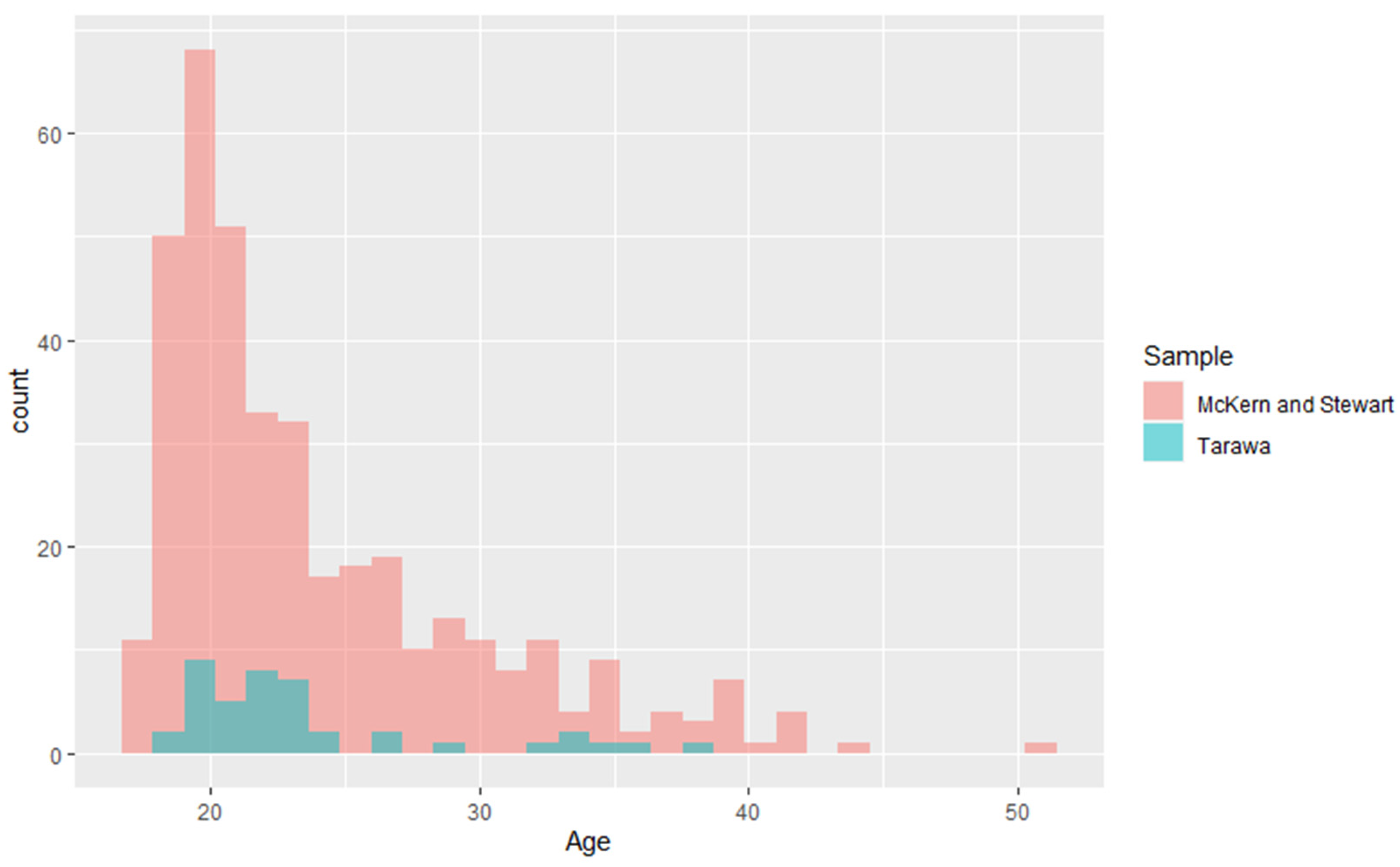
These data consist of 388 individuals from McKern and Stewart’s [25] sample and 41 recently identified individuals from the Battle of Tarawa. All individuals in this study are U.S. Service Members, lost during World War II or the Korean War, and are overwhelmingly young European American males (minimum age = 16 years 11 months, maximum age = 50 years 5 months, average age = 23 years 11 months). Figure 1 shows the age distribution of these samples.

Fourteen age indicators are used in this study (

Table 1. Age indicators used in this study.

Area/Element	Indicator
Clavicle	Medial Epiphysis
Pubic Symphysis	Dorsal Demiface
	Ventral Demiface
	Symphyseal Rim
Os Coxa	Ischiopubic Ramus
	Iliac Crest
Sacrum	S1/S2
	S2/S3
Scapula	Acromion
	Medial border
	Lateral border
Limbs	Proximal Humerus
	Distal Ulna
	Distal Radius
	Distal Femur
	Proximal Tibia
	Distal Fibula

). These comprise pubic symphysis morphology and epiphyseal fusion. Epiphyseal fusion is scored as no fusion (score of 0), beginning fusion (score of 1), active fusion (score of 3), and complete fusion (score of 4). Pubic symphysis morphology is assessed as three components, the dorsal demiface, the ventral demiface, and symphyseal rim. Each of these components are scored in six stages (0–5), with age progressing from 0 to 5.

Table 2. Description of pubic symphysis component stages.

Component	Description
Dorsal Demiface
Stage 0	Dorsal margin absent.
Stage 1	A slight margin formation first appears in the middle third of the dorsal border.
Stage 2	The dorsal margin extends along entire dorsal border.
Stage 3	Filling in of grooves and resorption of ridges to form a beginning plateau in the middle third of the dorsal demiface.
Stage 4	The plateau, still exhibiting vestiges of billowing, extends over most of the dorsal demiface.
Stage 5	Billowing disappears completely and the surface of the entire demiface becomes flat and slightly granulated in texture.
Ventral Demiface
Stage 0	Ventral beveling is absent.
Stage 1	Ventral beveling is present only at superior extremity of ventral border.
Stage 2	Bevel extends inferiorly along ventral border.
Stage 3	The ventral rampart begins by means of bony extensions from either or both of the extremities.
Stage 4	The rampart is extensive, but gaps are still evident along the earlier ventral border, most evident in the upper two-thirds.
Stage 5	The rampart is complete.
Symphyseal Rim
Stage 0	The symphyseal rim is absent
Stage 1	A partial dorsal rim is present, usually at the superior end of the dorsal margin; it is round and smooth in texture and elevated above the symphyseal surface.
Stage 2	The dorsal rim is complete and the ventral rim is beginning to form. There is no particular beginning site.
Stage 3	The symphyseal rim is complete. The enclosed symphyseal surface is finely grained in texture and irregular or undulating in appearance.
Stage 4	The rim begins to break down. The face becomes smooth and flat and the rim is no longer round but sharply defined. There is some evidence of lipping on the ventral edge.
Stage 5	Further breakdown of the rim (especially along superior ventral edge) and rarefaction of the symphyseal face. There is also disintegration and erratic ossification along the ventral rim.

provides the description of these stages from McKern and Stewart [25]. While scoring multiple areas of the pubic symphysis allows for higher fidelity in quantifying mosaic age changes to the symphyseal surface compared to phase-based methods, the original McKern and Stewart study estimated age from the pubic symphysis based on the composite score, or sum of the three components, which range from 0 to 15 [25]. Based on descriptive statistics and basic data visualization (plotting composite score against age), the authors found that some adjacent composite scores provided similar age estimates and were subsequently grouped together into a single category [25]. For example, composite scores of 11–13 have the same estimated age range of 23–39 years [25]. Thus, while in theory an individual with a composite score of 11 should be younger than an individual with a composite score of 13, the decision to group these composite scores together leads to each having a predicted age of 23–39 years.

This study tests the accuracy of conventional age estimation at the DPAA with a cohesive approach, where all relevant indicators are integrated into a single statistical model. Age estimation can be generalized by predicting a dependent variable from multiple dependent variables. Linear regression is a common method for prediction, but it is suboptimal for addressing age estimation, where a continuous variable is predicted by ordinal variables. Linear regression is an example of a parametric model, which are typically simpler and easier to interpret than their non-parametric counterparts. Parametric models, however, make fixed assumptions about the distribution of the underlying data and the relationship between the independent and dependent variables. These assumptions cannot be assumed in age estimation. Most importantly, the assumption of a linear relationship between the dependent variable age and the independent variables is violated in age estimation. Advanced parametric models, such as Bayesian regression, may overcome these assumption violations through explicitly defining the underlying prior distribution of each variable, including data transformations and interaction terms as extra parameters. A more parsimonious approach is to use a non-parametric model, which does not assume underlying variable distributions or the functional relationship between variables.

Random Forest Regression is an example of a non-parametric model and is the model used in this study. This model is a machine learning algorithm that grows prediction trees based on random subsets of the reference data, producing an ensemble of tree predictions. This process helps to reduce overfitting and define uncertainty around a prediction compared to a single tree estimate using all data. Random Forest Regression models are effective at analyzing non-linear relationships, such as predicting a continuous variable (i.e., age) from a set of ordinal variables (i.e., fusion scores) because each tree considers a subset of the variables and splits the data into multiple regions [29]. The RFR model used in this study trains the model using k-folds cross-validation based on the number of variables to arrive at an estimated optimal model, which is used to grow 1000 predictions (trees). The estimated age of an individual is defined by a point estimate and an uncertainty around that estimate, or 95% prediction interval. The point estimate is defined as the average of all 1000 predictions and the 95% prediction interval is defined by identifying the bottom 2.5% and top 97.5% of predicted ages. All statistical analyses are performed in R [30] and the Random Forest Regression model is from the Caret package [31].

For each of the Tarawa individuals, age is estimated using two RFR models. The first model is trained on the McKern and Stewart sample; the second model is trained on the McKern and Stewart sample and the Tarawa individuals minus the predicted individual. The results of each of these models are compared to the original FAR age intervals.

3. Results

Table 3. Comparison of age estimates to known age.

Ind.	Known Age	FAR Analysis *		McKern and Stewart *			Total Sample *
		Age	Interval	RF Est.	95% PI	Interval	RF Est.	95% PI	Interval
1	38.3	23–39	17	35.1	31–38	8	35.0	31–39	9
2	35.4	24–39	16	28.8	24–31	8	28.7	25–31	7
3	34.9	23–39	17	29.1	24–33	10	29.2	24–33	10
4	33.5	23–39	17	30.5	29–32	4	30.5	28–32	5
5	33.1	23–39	17	31.9	29–33	5	31.9	29–33	5
6	31.8	23–39	17	31.9	29–33	5	31.8	29–33	5
7	28.8	23–35	13	29.1	27–31	5	29.0	27–31	5
8	26.8	22–28	7	27.0	22–31	10	26.8	22–31	10
9	26.1	23–36	14	33.2	28–37	10	33.5	28–38	11
10	24.3	23–33	11	27.6	23–35	13	27.6	23–35	13
11	24.0	23–39	17	30.5	29–32	4	30.7	29–32	4
12	23.7	22–30	9	26.2	22–38	17	26.3	22–39	18
13	23.3	20–28	9	24.2	22–25	4	24.1	22–25	4
14	23.0	18–23	6	21.8	19–23	5	22.0	19–23	5
15	22.9	22–28	7	21.8	20–25	6	22.0	20–25	6
16	22.8	19–24	6	21.8	17–23	7	22.3	17–23	7
17	22.8	20–23	4	24.2	19–28	10	23.7	19–27	10
18	22.7	18–23	6	20.0	17–21	5	20.1	17–22	6
19	22.5	20–25	6	23.2	20–29	10	23.6	20–30	11
20	22.4	22–30	9	24.0	22–25	4	23.9	22–25	4
21	22.1	20–24	5	21.8	19–25	7	22.0	19–25	7
22	22.0	18–22	5	18.7	17–19	3	18.5	17–19	3
23	21.9	17–22	6	18.8	18–19	2	19.5	18–21	4
24	21.8	17–20	4	20.4	18–22	5	20.3	18–22	5
25	21.8	18–25	8	24.2	20–29	10	24.3	20–29	10
26	21.5	18–20	3	19.7	18–22	5	19.9	18–22	5
27	21.1	17–20	4	19.8	17–21	5	19.8	17–21	5
28	21.0	18–22	5	20.0	18–21	4	20.1	19–21	3
29	20.8	18–22	5	20.7	18–22	5	20.7	18–22	5
30	20.8	18–22	5	20.6	19–22	4	20.3	19–21	3
31	20.3	18–21	4	20.2	18–22	5	20.1	18–22	5
32	20.0	20–24	5	24.3	22–26	5	24.2	22–26	5
33	20.0	18–23	6	20.5	18–22	5	20.6	18–22	5
34	20.0	16–20	5	19.5	17–20	4	19.5	17–21	5
35	20.0	18–24	7	20.4	18–23	6	20.3	18–23	6
36	19.9	18–24	7	22.5	17–25	9	22.5	17–25	9
37	19.7	17–22	6	19.9	17–22	6	19.9	17–22	6
38	19.6	17–20	4	19.9	18–21	4	20.0	17–21	5
39	19.5	18–22	5	19.9	17–21	5	20.0	17–21	5
40	19.3	18–21	4	20.2	18–22	5	20.3	18–22	5
41	18.6	18–22	5	20.6	19–21	3	20.6	19–21	3

* Bold indicates the known age is outside of the estimated age interval.

compares the known age of each Tarawa individual to the FAR age estimates and the results of the two RFRs. The 95% prediction intervals for the RFR estimates are presented in year-level precision.

Table 4. Summary of age estimation performance.

	FAR Analysis	McKern and Stewart	Total Sample
Age Interval	8.1	6.3	6.4
Correct	38/41	31/41	33/41
% Correct	92.7%	75.6%	80.5%

provides aggregate summary information for the performance of the FAR analysis and each RFR model. Samples sizes for each prediction varied based on the variables used and data availability. Sample sizes range from 287 to 364 individuals, with an average of 314 individuals for the McKern and Stewart models and from 301 to 405 individuals, with an average of 334 individuals for the total sample (combined McKern and Stewart and Tarawa individuals) models.

Looking at accuracy, the FAR age estimates easily performed the best with 92.7% (38/41) of individuals falling within the age interval provided by the analyst, followed by 80.5% (33/41) for the total sample RFR, and 75.6% (31/41) for the McKern and Stewart RFR. The superiority in accuracy comes at a cost of precision, however, with the average predicted age interval of the FAR estimates being almost two years wider than the RFR models. This tradeoff between accuracy and precision is mainly relegated to the older individuals. The average age interval for the 11 oldest individuals is 14.6 years for FAR analysis and the RFR model interval is roughly half of that at 7.5 years. Of note, 10 of the 18 RFR mis-aged individuals fall within the 11 oldest (approximately the top 25%) individuals (see Table 3). All of these individuals were underaged by the RFR. There appears to be a general trend for under-aging, with all three incorrect FAR age estimates and 12 of the 18 incorrect RFR age estimates under aging individuals.

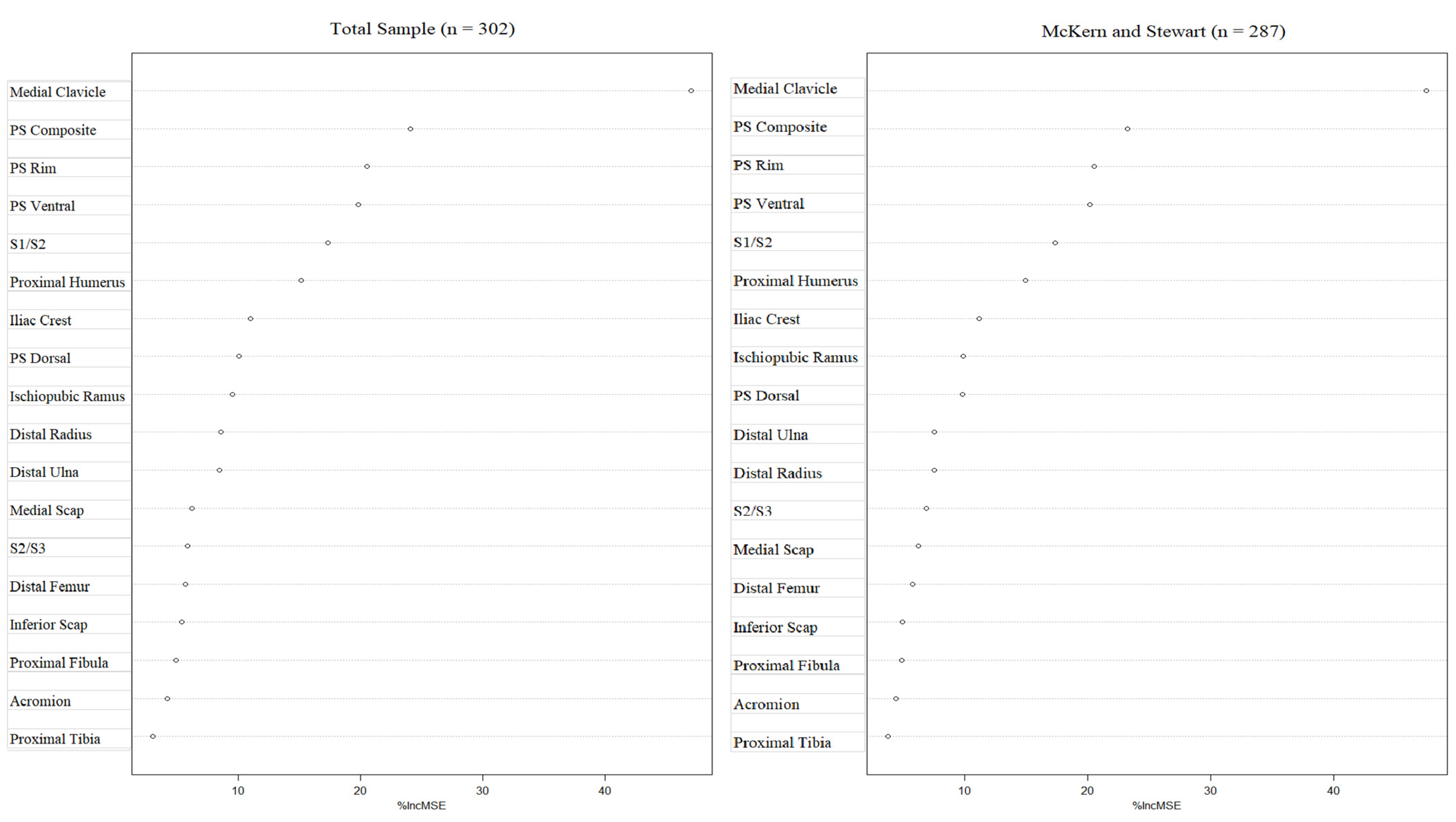
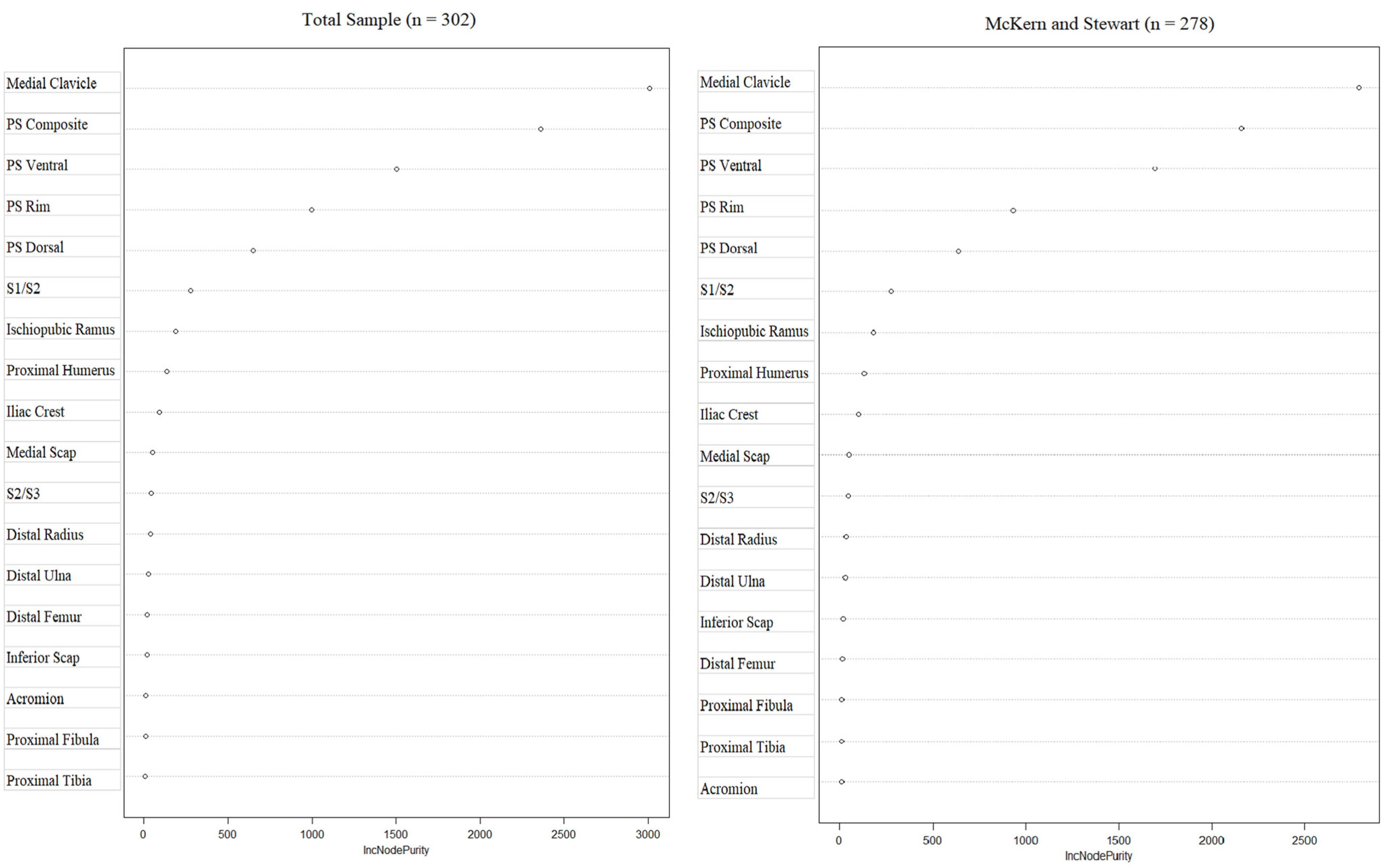
Examining the RFR models in more detail reveals both are essentially the same in terms of variable importance (Figure 2 and Figure 3). Figure 2 illustrates the effect of substituting a variable for noise on the prediction of age. The longer the variable bar in Figure 2, the more error is introduced into the model when substituting that variable for randomness. Stated another way, the longer the bar in Figure 2, the more informative that variable is for age estimation. A similar understanding can be taken from Figure 3. Random Forest Models arrive at a prediction through data partitioning. The more informative a variable is to age, the more likely it is to partition these data. And node purity is a measure of how well data are partitioned while minimizing overlap.

The difference in age accuracy in the RFR that includes the McKern and Stewart and Tarawa data over the RFR based on only the McKern and Stewart data is likely a result of increased sample size and variation in trait scoring reflecting current analyses at the DPAA. Age estimation is mainly driven by late-fusing epiphyses, such as the medial clavicle, the first and second sacral vertebrae, and the pelvis; and the pubic symphysis, which shows a combination of degenerative and developmental morphology (see Figure 2 and Figure 3).

4. Discussion

These results highlight several important concepts in the application of biological anthropology and other fields that deal with the practical aspects of uncertainty in estimation. First, the RFR used in this study has the common issue of estimation bias in age estimation, where older individuals are under-aged and younger individuals are over-aged, with the former especially true in the current study [32,33]. Three of the four oldest individuals were incorrectly aged by the RFR model, which represents one fourth of the incorrect ages. Stated another way, the top 10% in age were incorrectly under-aged 75% of the time and this represented 25% of the incorrect ages. And 56% of mis-aged individuals were the oldest 25% of individuals, and they were all underaged. The bias in this study would likely not benefit from an explicit Bayesian approach of an informative prior age distribution [34]. And may be better understood as a non-uniform distribution of the reference data, where RFR and other statistical models have more information in the middle of the reference distribution [35]. As Figure 1 shows, the age distribution of these individuals is strongly skewed younger. Interestingly, the distribution from which the Tarawa individuals are drawn from is essentially a smaller version of the McKern and Stewart sample. This observation suggests that applying a prior distribution to age estimation models will not alleviate the issue of bias observed in this study. Rather, this issue may be the result of the information the model has to work with, suggesting a uniform age distribution for reference samples would be optimal. As skeletal biologists, our samples are what they are. Often, the samples available to skeletal biologists are biased subsets of our target populations, the unknown individuals on which our methods are applied. We cannot manifest a uniform age distribution for our reference samples. We may, however, be able to simulate one. This idea, at first, may sound like statistical jargon to many, but it is an avenue worth exploring. The design and implementation are beyond the scope of this article, but it is possible to simulate reference data based on known relationships from observed data in a scientifically rigorous manner to construct a uniform reference sample distribution. Additionally, supplementing data sets with simulated data could have the additional benefit of capturing variation not observed in the sample population but found in the target population, or the population ‘at large’ that we assume our reference samples to approximate. Exploring the utility of data simulation in age estimation would build on recent research in computational modeling and trait choice [36].

A discussion point more particular to this study is the construction of age estimates. The methodology of constructing age estimates through the use of descriptive statistics and basic data visualization used by McKern and Stewart [25] is historically pervasive in forensic anthropology [7,8,9,10,11,12]. This prevalence is understandable for two reasons. First, it is the nature of age phases or the choice to reduce composite methods to a single composite score. The former is one variable and the latter consolidates multiple variables into one. Both reduce morphological age-related information into a single variable. Descriptive statistics and basic data visualization are the only tools available when dealing with a single variable. As such, age estimates are limited to the mean age of the phase/composite score and some expression of variability around that score (e.g., standard deviation and observed age range). These are rather blunt statistical tools for addressing age estimation. This assertion is supported by the large age intervals (to the point they are of questionable practical utility) provided by these methods [7,8,9,10,11,12]. The second reason is the historic difficulty in employing advanced statistical frameworks for questions in forensic anthropology. At the time of McKern and Stewart’s study, computers filled rooms and were programmed by punch-cards. It is understandable that their analysis was rudimentary by modern standards. This is not an indictment of previous age estimation research in forensic anthropology. It is the natural progression of the field. An in-depth understanding of modern, advanced statistical modeling and the programming ability to implement them have not traditionally been part of the forensic anthropologists’ knowledge base. In fact, the ability of researchers to develop and deploy modern statistical modeling is a recent development.

As mentioned in the introduction, the general guidance at the DPAA for defining an age interval based on several age indicators is to define the lower-bound based on the oldest lower-bound among age indicators and the upper-bound is the youngest upper-bound among age indicators. Another common practice, especially in individuals that exhibit skeletal maturity, is to take the age range provided by McKern and Stewart based on their groupings of component scores. By summing the scores for the three components of the pubic symphysis, McKern and Stewart grouped variations. This variation-consolidation is further compounded by grouping composite scores together into set age ranges. This is obvious in the repetitive use of FAR age ranges. The common 23–39 years age prediction (see Table 3 and Materials and Methods), for example, is the age range provided by McKern and Stewart for total pubic symphysis component scores of 11–13 [25]. At first glance, this would appear to be a rudimentary approach, but it certainly is effective. It is true that basing pubic symphysis age on the grand component score loses fidelity in age-related morphology. This approach, perhaps more importantly, hides errors derived from interobserver variability in scoring. Of the 125 possible combinations of scores for the three traits, only 21 were observed by McKern and Stewart (25:83). All 41 of the Tarawa individuals had complete pubic symphysis scores. Of those 41 scores, eight (~20%) were in combinations not observed by McKern and Stewart. This finding suggests pubic symphysis variability in current case work not observed in the McKern and Stewart sample, interobserver variability or error in scoring, or ambiguity in score definitions. While it is almost certainly a combination of all three, ambiguity in trait definitions is obvious to most practitioners familiar with the method. This ambiguity extends to epiphyseal fusion scores as well. While some traits are well-described, such as the fusion of the iliac crest, many are not, such as that for the ischiopubic ramus, which logically leads to observer error. Given that the fidelity of these ordinal variables is low, with only four possibilities, a score difference in a couple of traits will compound in the resulting age estimate from a statistical model such as RFR. This difference between McKern and Stewart’s understanding of their method and how it is understood by current analysts is suggested by the increased accuracy from the RFR that incorporates both the McKern and Stewart data and cases from current analysts. There was a 5% increase in accuracy, with a near-identical level of precision by adding just over 10% modern case work to the McKern and Stewart sample.

This study shows the effectiveness of current age estimation at the DPAA. This is due in large part to the efforts of McKern and Stewart and their 1957 study. And while the RFR models used in this study show promise, they cannot be recommended over current practices based on the results of this study. This study also highlights important areas for improvement both at the DPAA and within the larger field of forensic anthropology. These include the need for refined methodologies that are easy to correctly implement, studies that incorporate multiple age indicators into a single model, and the need for more data and how we understand and construct our reference samples.

References

- Blau, S.; Ubelaker, D.H. (Eds.) Handbook of Forensic Anthropology and Archaeology; Routledge: New York, NY, USA, 2016. [Google Scholar]
- Christensen, A.M.; Passalacqua, N.V.; Bartelink, E.J. Forensic Anthropology: Current Methods and Practice; Elsevier Inc.: San Diego, CA, USA, 2014. [Google Scholar]
- Latham, K.E.; Finnegan, M. (Eds.) Age Estimation of the Human Skeleton; Charles C. Thomas: Springfield, IL, USA, 2010. [Google Scholar]
- Rogers, T.L. Skeletal age estimation. In Handbook of Forensic Anthropology and Archaeology; Blau, S., Ubelaker, D.H., Eds.; Routledge: New York, NY, USA, 2016; pp. 273–292. [Google Scholar]
- Todd, T.W. Age changes in the pubic bone I. The male white pubis. Am. J. Phys. Anthropol. 1920, 3, 285–334. [Google Scholar] [CrossRef]
- Todd, T.W. Age changes in the pubic bone. Am. J. Phys. Anthropol. 1921, 4, 1–77. [Google Scholar] [CrossRef]
- Katz, D.; Suchey, J.M. Age determination of the male os pubis. Am. J. Phys. Anthropol. 1986, 69, 427–435. [Google Scholar] [CrossRef]
- Berg, G.E. Pubic bone age estimation in adult women. J. Forensic Sci. 2008, 53, 569–577. [Google Scholar] [CrossRef]
- Hartnett, K.M. Analysis of age at death estimation using data from a new, modern autopsy sample—Part I: Pubic bone. J. Forensic Sci. 2010, 55, 1145–1151. [Google Scholar] [CrossRef]
- Lovejoy, C.O.; Meindl, R.S.; Pryzbeck, T.R.; Mensforth, R.P. Chronological metamorphosis of the auricular surface of the ilium: A new method for the determination of adult skeletal age at death. Am. J. Phys. Anthropol. 1985, 68, 15–28. [Google Scholar] [CrossRef]
- Buckberry, J.L.; Chamberlain, A.T. Age estimation from the auricular surface of the ilium: A revised method. Am. J. Phys. Anthropol. 2002, 119, 231–239. [Google Scholar] [CrossRef]
- Osborne, D.L.; Simmons, T.L.; Nawrocki, S.P. Reconsidering the auricular surface as an indicator of age at death. J. Forensic Sci. 2004, 49, 905–911. [Google Scholar] [CrossRef]
- Boldsen, J.L.; Milner, G.R.; Konigsberg, L.W.; Wood, J.W. Transition analysis: A new method for estimating age from skeletons. In Paleodemography: Age Distributions from Skeletal Samples; Hoppa, R.D., Vaupel, J.W., Eds.; Cambridge University Press: Cambridge, UK, 2002; pp. 73–106. [Google Scholar]
- Getz, S.M. The use of transition analysis in skeletal age estimation. Wiley Interdiscip. Rev. Forensic Sci. 2020, 2, c1378. [Google Scholar] [CrossRef]
- Garvin, H.M.; Passalacqua, N.V. Current practices by forensic anthropologists in adult skeletal age estimation. J. Forensic Sci. 2013, 57, 427–433. [Google Scholar] [CrossRef] [PubMed]
- Ubelaker, D.H.; Khosrowshahi, H. Estimation of age in forensic anthropology: Historical perspective and recent methodological advances. Forensic Sci. Res. 2019, 4, 1–9. [Google Scholar] [CrossRef] [PubMed]
- Katz, D.; Suchey, J. Race differences in pubic symphyseal aging patterns in the male. Am. J. Phys. Anthropol. 1989, 80, 167–172. [Google Scholar] [CrossRef]
- Hoppa, R.D. Population variation in osteological aging criteria: An example from the pubic symphysis. Am. J. Phys. Anthropol. 2000, 111, 185–191. [Google Scholar] [CrossRef]
- Langley-Shirley, N.; Jantz, R.L. A Bayesian approach to age estimation in modern Americans from the clavicle. J. Forensic Sci. 2010, 55, 571–583. [Google Scholar] [CrossRef]
- Suchey, J.M. Problems in the aging of females using the os pubis. Am. J. Phys. Anthropol. 1979, 51, 467–470. [Google Scholar] [CrossRef]
- Suchey, J.M.; Brooks, S.T.; Katz, D. Instructions for use of the Suchey-Brooks system for age determination of the female os pubis. In Instructional Materials Accompanying Female Pubic Symphysial Models of the Suchey-Brooks System; France Casting: Fort Collins, CO, USA, 1988. [Google Scholar]
- Bello, S.M.; Thomann, A.; Signoli, M.; Dutour, O.; Andrews, P. Age and sex bias in the reconstruction of past population structures. Am. J. Phys. Anthropol. 2006, 129, 24–38. [Google Scholar] [CrossRef] [PubMed]
- Scheuer, L.; Black, S. Developmental Juvenile Osteology, 1st ed.; Academic Press: New York, NY, USA, 2000. [Google Scholar]
- Schaefer, M.C.; Black, S.M. Comparison of ages of epiphyseal union in north American and Bosnian skeletal material. J. Forensic Sci. 2005, 50, 777–784. [Google Scholar] [CrossRef] [PubMed]
- McKern, T.W.; Stewart, T.D. Skeletal Age Changes in Young American Males; Technical Report EP-45; Quartermaster Research and Development Command: Natick, MA, USA, 1957; Available online: https://apps.dtic.mil/sti/citations/AD0147240 (accessed on 2 March 2022).
- Wilson, E.K. A125: A reanalysis of Korean War anthropological records to support the resolution of cold cases. In Proceedings of the American Academy of Forensic Sciences, Las Vegas, NV, USA, 22–27 February 2019; Peat, M.A., Ed.; American Academy of Forensic Sciences: Colorado Springs, CO, USA, 2019; pp. 189–196. [Google Scholar]
- Taylor, R.J.; Scott, A.L.; Koehl, A.J.; Trask, W.R.; Maijanen, H. The Tarawa Project Part I: A multidisciplinary approach to resolve commingled human remains from the Battle of Tarawa. Forensic Anthropol. 2019, 2, 87–95. [Google Scholar] [CrossRef]
- Defense POW/MIA Accounting Agency. Battle of Tarawa. Available online: https://dpaa-mil.sites.crmforce.mil/dpaaFamWebInTarawa (accessed on 20 February 2023).
- Breiman, L. Random forest. Mach. Learn. 2001, 45, 5–32. [Google Scholar] [CrossRef]
- R Core Team. R. A Language and Environment for Statistical Computer, R Foundation for Statistical Computing: Vienna, Austria, 2021. Available online: https://www.R-project.org/(accessed on 30 January 2023).
- Kuhn, M. Building Predictive Models in R Using the caret Package. J. Stat. Softw. 2008, 28, 1–26. [Google Scholar] [CrossRef]
- Hoppa, R.D.; Vaupel, J.W. The Rostock Manifesto for paleodemography: The way from stage to age. In Paleodemography: Age Distributions from Skeletal Samples; Hoppa, R.D., Vaupel, J.W., Eds.; Cambridge University Press: Cambridge, UK, 2002; pp. 1–8. [Google Scholar]
- Hoppa, R.D.; Vaupel, J.W. Paleodemography: Age Distributions from Skeletal Samples; Cambridge University Press: Cambridge, UK, 2002. [Google Scholar]
- Konigsberg, L.W. Multivariate cumulative probit for age estimation using ordinal categorical data. Ann. Hum. Biol. 2015, 42, 368–378. [Google Scholar] [CrossRef] [PubMed]
- Usher, B.M. Reference samples: The first step in linking biology and age in the human skeleton. In Paleodemography; Hoppa, R.D., Vaupel, J.W., Eds.; Cambridge University Press: Cambridge, UK, 2018; pp. 29–47. [Google Scholar]
- Navega, D.; Costa, E.; Cunha, E. Adult Skeletal Age-at-Death Estimation through Deep Random Neural Networks: A New Method and Its Computational Analysis. Biology 2022, 11, 532. [Google Scholar] [CrossRef] [PubMed]
Figure 1.
The age distribution of the McKern and Stewart sample and Tarawa individuals.
Figure 2.
The increase in mean square error (x-axis) by random permutation of variables (y-axis) in the total model. Variables are sorted along the y-axis in descending order of mean square error increase. The higher the mean square error, the more important a variable is for age estimation.
Figure 3.
Increase in node purity (x-axis) by variable (y-axis) inclusion in the total model. Variables are sorted along the y-axis in descending order of node purity increase. The higher the increase in node purity, the more important a variable is for age estimation.